Article

Sine Cosine Algorithm Assisted FOPID Controller Design for Interval Systems Using Reduced-Order Modeling Ensuring Stability

1
Electrical Engineering, National Institute of Technology Raipur, Chhattisgarh 492010, India
2
Electrical and Electronics Engineering, ABES Engineering College, Ghaziabad 201009, India
3
Electrical Engineering, Malaviya National Institute of Technology Jaipur, Rajasthan 302017, India
*
Authors to whom correspondence should be addressed.
Algorithms 2020, 13(12), 317; https://doi.org/10.3390/a13120317
Submission received: 18 October 2020 / Revised: 22 November 2020 / Accepted: 23 November 2020 / Published: 1 December 2020
(This article belongs to the Special Issue Metaheuristic Algorithms in Engineering Optimization Problems)

Abstract

:
The focus of present research endeavor was to design a robust fractional-order proportional-integral-derivative (FOPID) controller with specified phase margin (PM) and gain cross over frequency ( ω g c ) through the reduced-order model for continuous interval systems. Currently, this investigation is two-fold: In the first part, a modified Routh approximation technique along with the matching Markov parameters (MPs) and time moments (TMs) are utilized to derive a stable reduced-order continuous interval plant (ROCIP) for a stable high-order continuous interval plant (HOCIP). Whereas in the second part, the FOPID controller is designed for ROCIP by considering PM and ω g c as the performance criteria. The FOPID controller parameters are tuned based on the frequency domain specifications using an advanced sine-cosine algorithm (SCA). SCA algorithm is used due to being simple in implementation and effective in performance. The proposed SCA-based FOPID controller is found to be robust and efficient. Thus, the designed FOPID controller is applied to HOCIP. The proposed controller design technique is elaborated by considering a single-input-single-output (SISO) test case. Validity and efficacy of the proposed technique is established based on the simulation results obtained. In addition, the designed FOPID controller retains the desired PM and ω g c when implemented on HOCIP. Further, the results proved the eminence of the proposed technique by showing that the designed controller is working effectively for ROCIP and HOCIP.

1. Introduction

In practical applications, many small modules are congregated to form a major dynamic system. The study, simulation and comprehensive analysis of such dynamic systems are carried out by means of mathematical modeling [1,2]. The derived mathematical models for such congregated systems, generally, turn out to be complex involving higher order transfer functions. The practical examples of higher order systems are as follows: nuclear reactors, power systems, chemical plants, etc. The controller design becomes a bit challenging for control engineers in these cases since the order of system is high [3]. In these cases, approximation of high-order transfer functions is advised to ease the controller design process [4,5]. The benefits of approximation include reduction in computational complexity, simplified understanding of system and minimization in cost while designing hardware for the controller [6,7].
In industrial control applications, a proportional-integral-derivative (PID) controller is more popular. PID controller is used extensively due to its simple form and good performance. For tuning the gains of PID controllers, a large number of methods/algorithms have been developed in the literature. Over time, a significant development in fractional calculus is seen. Several studies have demonstrated the capabilities of fractional calculus in the field of pure mathematics [8,9], engineering [10,11], biological engineering [12] and physics [13]. It motivated the development of designing fractional order systems and controllers as far as control theory is concerned [14,15].
Many good articles are presented in the literature on the design of fractional-order PID (FOPID) controllers [16,17]. FOPID controller involves an additional pair of parameters (integral order and differential order) over an integer-order PID (IOPID) controller. These parameters provide better control if tuned properly. Similarly, these additional parameters are also seen as helpful in designing a system having robustness against high frequency noise signals, better disturbance rejection, etc. [18]. In [19], an FOPID controller is developed for fractional-order systems to achieve better performance over IOPID. An FOPID controller is designed for a five bar linkage robot based on modified PSO algorithm by Aghababa [20]. In [21], the robust stability analysis of fractional-order interval systems with multiple time delays and neutral systems is investigated.
Fractional integral-fractional derivative controller using small gain theorem and sensitivity function analysis to achieve desired PM and ( ω g c ) is discussed by Azarmi et al. [22]. Liu and Zhang [23] designed an FOPID controller based on the Bode optimal reference model and flat phase property that ensures desired transient performance characteristics. This design is also robust to system parameter variations. Similarly, Saidi et al. [24] developed three new constrained numerical optimization algorithms for tuning the parameters of FOPID controller for delay-systems and parameter uncertain systems. In this case, it is seen that the property of iso-damping is enhanced. Bhookya et al. [25] proposed an FOPID controller based on the sine-cosine algorithm (SCA) optimization technique [26] for an automatic voltage regulator (AVR) system. Results showed that SCA tuned FOPID controller performance is superior in improving the transient response and is robust to external disturbance. An FOPID controller using SCA is designed to handle issues likes fluctuations in load and frequency, discontinuous power flow from wind turbines, etc. in a hybrid two-area power system by Khezri et al. [27].
Various strategies are available for model order reduction of higher order continuous and discrete interval systems. In [28], the low-order interval model is obtained using the stability equation technique, Kharitonov’s theorem and minimization of integral-square-error (ISE) utilizing the differential evolution optimization technique. Singh et al. [29] adopted Routh–Pade approximation for order reduction of interval systems and also proposed two simple expressions for computing time moments (TMs) and Markov parameters (MPs). A thorough literature survey on model order reduction (MOR) methods based on Routh approximation for discrete and continuous interval systems is given in [30]. Later, the order reduction of higher order continuous interval systems is carried out using frequency domain reduction techniques [31] where the denominator of the model is derived from a differentiation method and the numerator is achieved using factor division, differentiation and Pade approximation methods. Another concept of order reduction of interval systems is stated depending on ISE minimization and impulse response energy using modified particle swarm optimization (PSO) algorithm by Anand et al. [32].
Model order reduction of linear time-invariant continuous and discrete interval systems based on Kharitonov’s theorem using the differential method was presented by Potturu and Prasad [33]. The resulting interval model preserves all the dominant characteristics of original interval system. The frequency domain fractional-order controllers are designed generally based on the specifications [34] like phase margin, gain crossover frequency, steady-state error cancellation, high-frequency noise rejection and good output disturbance rejection. Authors in [35] extended the differentiation method for reduced order modeling where the stability of lower order models is always guaranteed. In addition, it retains the initial TMs of higher order systems. Further, a new approach of order reduction based on the concept of impulse response gramian is developed in the frequency domain in [36]. Recently, Dewangan et al. [37] proposed a multipoint Routh–Pade approximation technique for single-input-single-output (SISO) and multi-input-multi-output (MIMO) interval systems. These methods assure a stable reduced model for higher order continuous interval systems.
This research presents a design of a robust fractional-order proportional-integral-derivative (FOPID) controller for reduced-order continuous interval plant (ROCIP) of higher-order continuous interval plant (HOCIP) based on considered frequency domain specifications using an advanced sine-cosine algorithm (SCA). Later, this controller is cascaded with HOCIP. Here, PM and ω g c are considered as performance criteria of HOCIP for tuning the five parameters of FOPID controller. Since the design of the controller is done in the frequency domain, this approach guarantees the robustness and stability of the system. An improved Routh–Pade approximation method is utilized for reduced order modeling of HOCIP. The modified Routh table is utilized to derive the denominator polynomial of interval model whereas the coefficients of numerator polynomial are obtained by matching few TMs and MPs of system with those of the model. This order reduction technique always yields stable ROCIPs for stable HOCIPs. A third order interval plant is considered as an example to demonstrate the whole procedure of FOPID controller tuning and model order reduction. The efficiency of the proposed method for design of the FOPID controller is proved from the simulation results obtained.
The article is structured into seven sections: Section 1 includes the detailed literature survey on the present investigation. The preliminaries of fractional calculus and the structure of FOPID controller are given in Section 2. Problem formulation is briefed in Section 3. The design procedure for the proposed FOPID controller is illustrated in Section 4. In Section 5, the order reduction method for HOCIP is presented. Section 6 explains the SCA in detail. Section 7 includes the test case and its simulation results. Finally, the conclusions are reported in Section 8.

2. Preliminaries

2.1. Fractional Order Calculus

Recently, many systems are modeled as fractional-order systems utilizing fractional-order calculus. The fractional-calculus is found in several applications [34] in areas including electromagnetic waves [38], chemical engineering [39], signal processing [40], polymer science [41], electro-chemistry [42], neural networks [43], fluid mechanics [44], bio-engineering and bio sciences [45], control of power electronics [46], nonlinear control [47], etc.
The generalization of the integration and differentiation operators in fractional calculus [48] of k t h order is defined as
p D q k = { d k d t k k   > 0 1 k   = 0 p q d τ k k   < 0
where p and q are the limits of the operation. The integration and differentiation of any real order can be performed. The Riemann–Liouville formula [49] for differentiation is given as
p D q k f ( t ) = 1 Γ ( n k ) d n d t n p q f ( τ ) ( t τ ) k n + 1 d τ
where k can be any value in-between ( n 1 ) and n, and Γ ( . ) is a Gamma function.
The Grünwald–Letnikov’s definition of the fractional-order derivative [34] is expressed as
p D q k f ( t ) = lim h 0 h k a = 0 ( q p ) h ( 1 ) a k a f ( t a h )
where 1 a k a are the binomial coefficients C a k , a = 0 , 1 , ; and . denotes the integer part. The formula given in [48] can be utilized to calculate the binomial coefficients.
The other commonly used formula for differentiation is known as Caputo expression [48]. The Caputo expression is defined as
p D q k f ( t ) = 1 Γ ( n k ) p q f n ( τ ) ( t τ ) k n + 1 d τ
where ( n 1 ) < k < n .

2.2. Fractional-Order PID (FOPID) Controller

The general formula for an FOPID controller [50] is depicted as
C ( s ) = K a + K b s α + K c s β
which is commonly referred to as P I α D β controller where K a , K b , K c are the proportional, integral and derivative gains, respectively. The parameters α and β indicate the positive real numbers [51]. In most of the engineering applications [23,50,52] the typical range of α and β variables lies with in ( 0 , 2 ) while designing FOPID controller. The primary benefits of the FOPID controller are achieved with extra tuning parameters namely α (non-integer order of integrator) and β (non-integer order of differentiation) as compared to conventional PID controller. As a result of these additional two parameters, FOPID controllers can be tuned in such a way that these may produce better control [53].

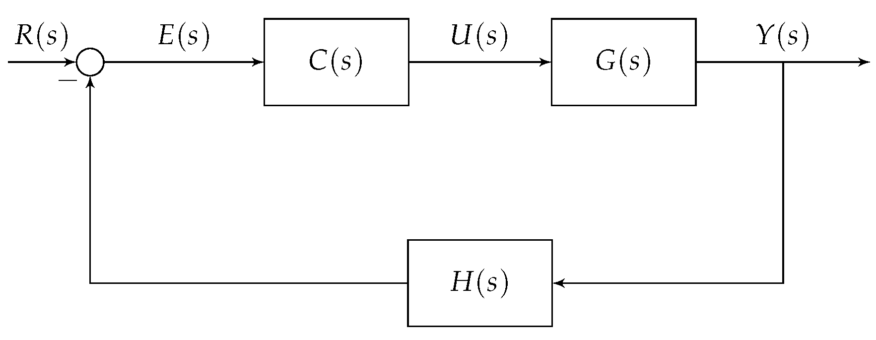
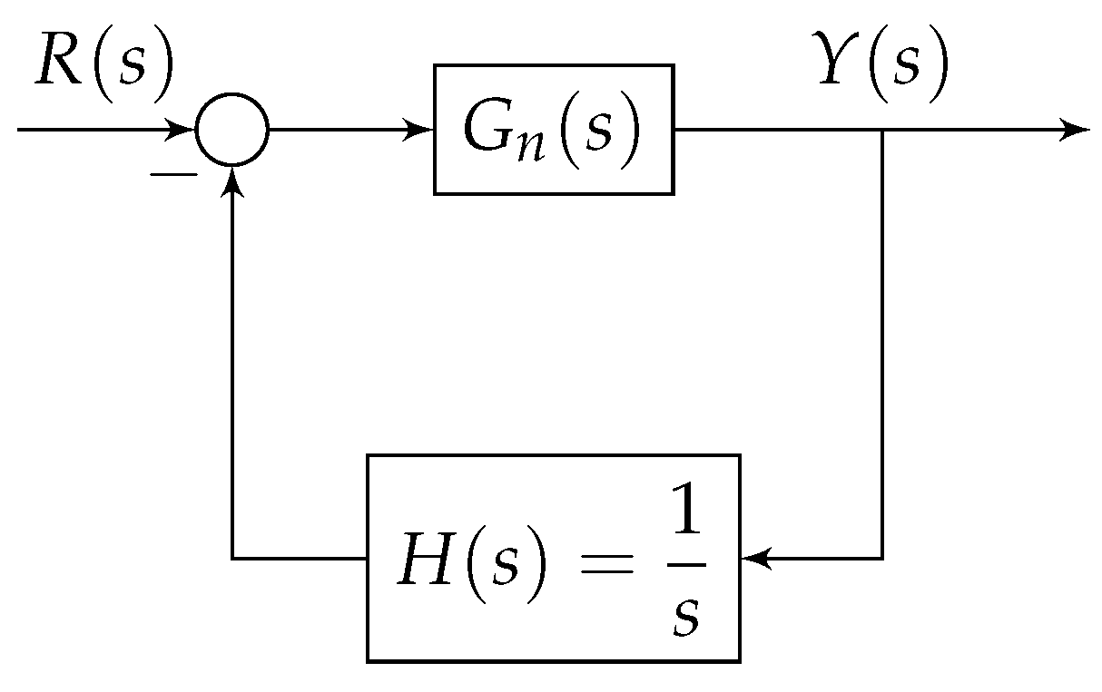
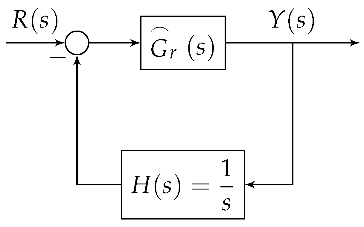
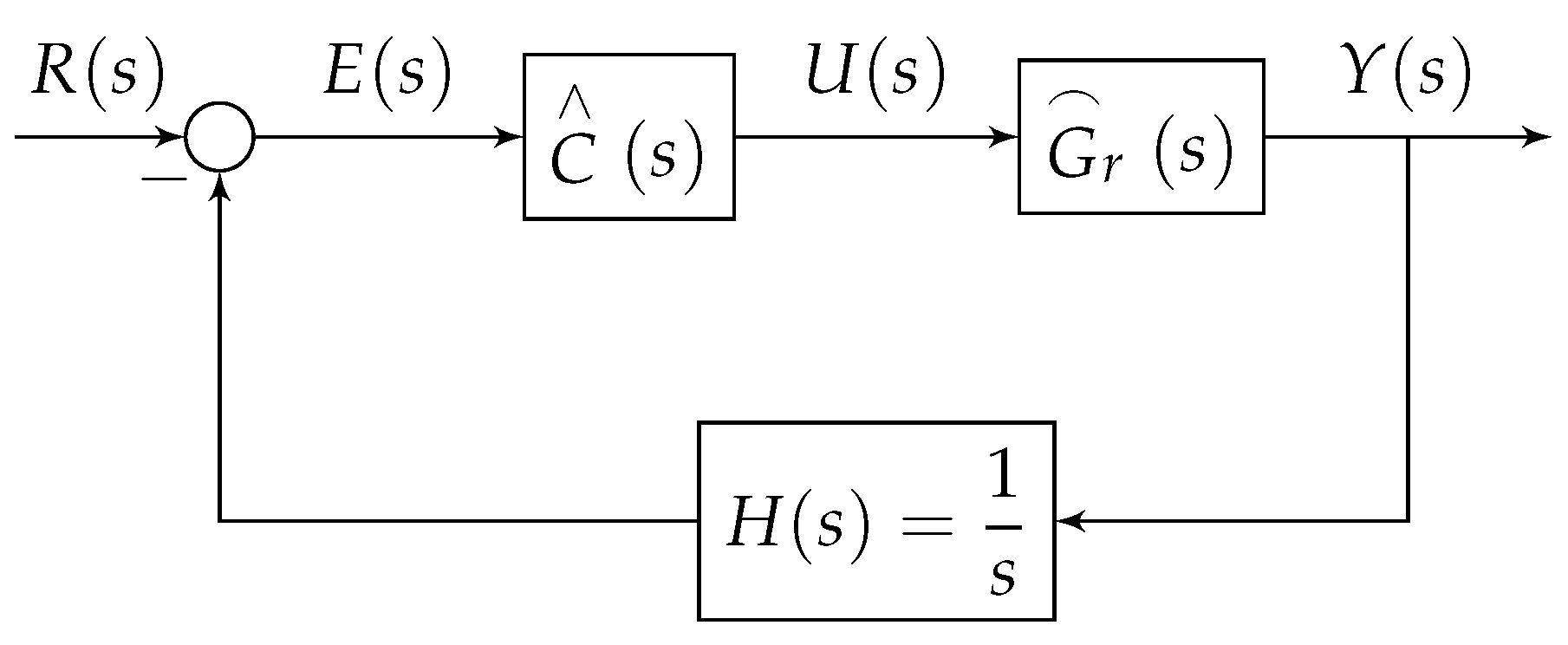
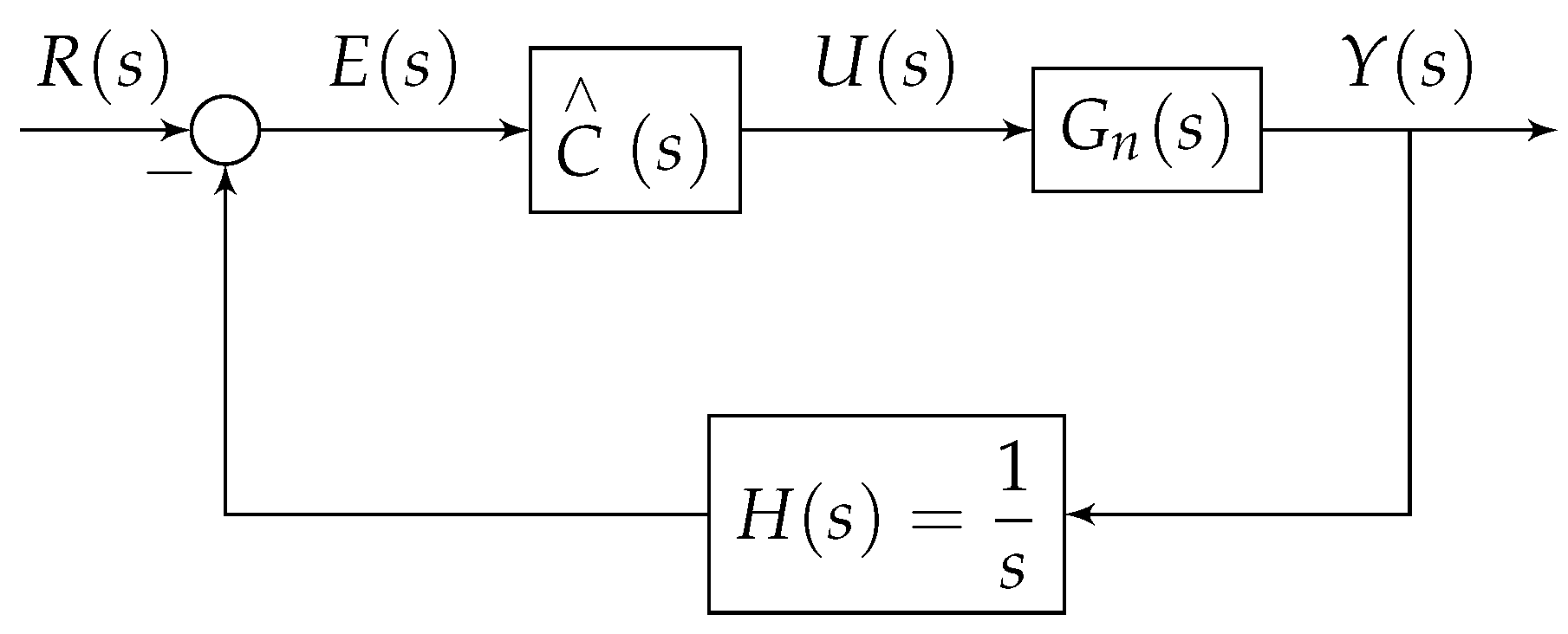
3. Problem Formulation

Suppose, an nth-order SISO continuous interval plant G n ( s ) for the closed-loop control system [54] of Figure 1 is expressed as
G n ( s ) = A ( s ) B ( s ) = [ A 0 , A 0 + ] + + [ A n 1 , A n 1 + ] s n 1 [ B 0 , B 0 + ] + [ B 1 , B 1 + ] s + + [ B n , B n + ] s n
The interval coefficients of numerator polynomial A ( s ) are [ A i , A i + ] for ( i = 0 , 1 , , n 1 ) , with A i + as upper bounds and A i as lower bounds, respectively. Likewise, interval coefficients of denominator polynomial B ( s ) are [ B i , B i + ] for ( i = 0 , 1 , , n ) , with B i + as upper bounds and B i as lower bounds, respectively. The power series [55] form of HOCIP, (6), about s = 0 and s = , respectively, are expressed as
G n ( s ) = λ 0 + λ 1 s + + λ k s k +
G n ( s ) = μ 1 s 1 + μ 2 s 2 + + μ k s k +
where λ i = [ λ i , λ i + ] for i = 0 , 1 , 2 , and μ i = [ μ i , μ i + ] for i = 1 , 2 , 3 , are TMs and MPs of the interval system, respectively.
Figure 2 represents the closed-loop system without an FOPID controller. Figure 3 depicts the reduced-order model G r s of HOCIP in place of G n ( s ) . The desired reduced-order continuous interval plant (ROCIP) G r s of G n ( s ) is represented as
G r ( s ) = E ( s ) F ( s ) = [ e 0 , e 0 + ] + [ e 1 , e 1 + ] s + + [ e r 1 , e r 1 + ] s r 1 [ f 0 , f 0 + ] + [ f 1 , f 1 + ] s + + [ f r , f r + ] s r
where r < n . The interval coefficients of numerator polynomial E ( s ) are [ e i , e i + ] for ( i = 0 , 1 , , r 1 ) , with e i + as upper bounds and e i as lower bounds, respectively. Similarly, the interval coefficients of denominator polynomials F ( s ) are [ f i , f i + ] for ( i = 0 , 1 , , r ) with f i + as upper bounds and f i as lower bounds, respectively. The model, (9), is expressed as
G r ( s ) = λ 0 + λ 1 s + + λ k s k + ( expansion about s = 0 )
G r ( s ) = μ 1 s 1 + μ 2 s 2 + + μ k s k + ( expansion about s = )
where λ i = λ i , λ i + for i = 0 , 1 , 2 , and μ i = μ i , μ i + for i = 1 , 2 , , 3 , are TMs and MPs of ROCIP.
The model G r s in Figure 3 is an approximation of system G n ( s ) in Figure 2 which is obtained by order reduction technique. In this work, the denominator of G r s is obtained from improved Routh approximation [56] and numerator of G r s is derived by matching of TMs and MPs [29]. Figure 4 shows the closed-loop control system with FOPID controller C ( s ) designed for ROCIP. Once the design for ROCIP is established, the same controller is applied to HOCIP as depicted in Figure 5 in order to ensure the applicability of designed controller for original system.

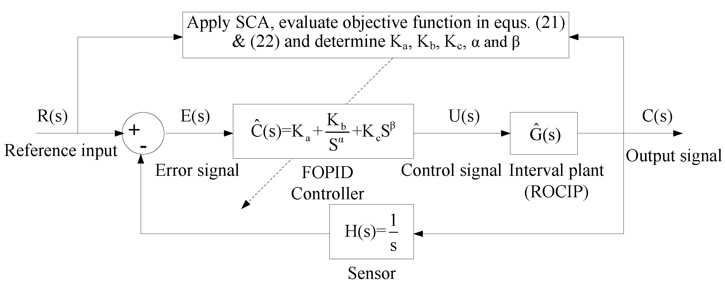
4. Design of FOPID Controller

The procedure to design an FOPID controller ( P I α D β ) for ROCIP to meet the desired performance is discussed in this section. The ROCIP of first order for (9) is given as
G 1 ( s ) = [ e 0 , e 0 + ] [ f 0 , f 0 + ] + [ f 1 , f 1 + ] s
where e 0 and e 0 + , respectively, are lower and upper limits of interval coefficient [ e 0 , e 0 + ] of the numerator of G 1 ( s ) . Similarly, f 0 and f 1 are lower limits, and f 0 + and f 1 + are upper limits of interval coefficients [ f 0 , f 0 + ] and [ f 1 , f 1 + ] .
The five unknown parameters of P I α D β controller are determined to satisfy the criteria of specified PM and ω g c . These unknown design parameters of P I α D β controller are estimated by solving two non-linear equations [10,57,58]. The expressions given in (13) and (14) should be satisfied for a specified phase margin and gain crossover frequency [59].
20 log 10 | C ( j ω g c ) G ( j ω g c ) H ( j ω g c ) | = 0
A r g C ( j ω g c ) G ( j ω g c ) H ( j ω g c ) = π + ϕ p m

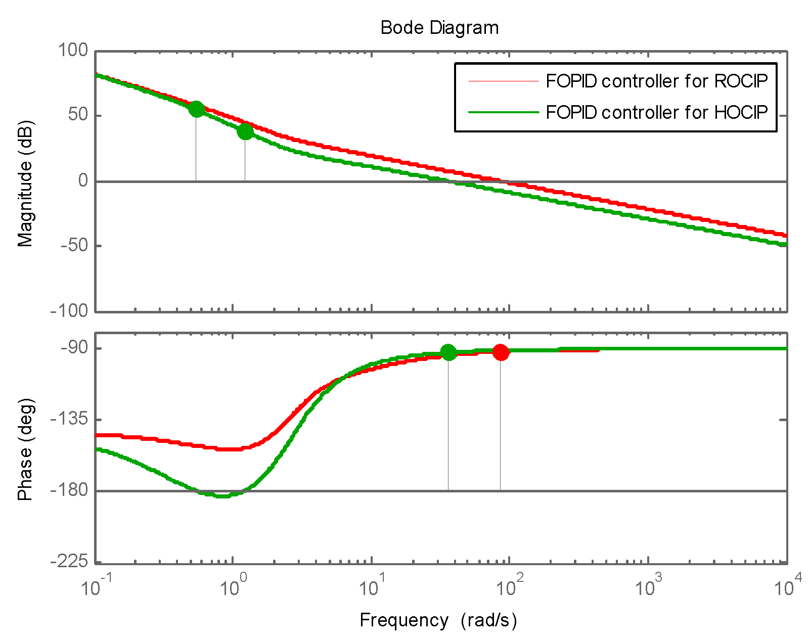
4.1. Description of Fractional Order Controller Based on Bode Envelope

The transfer functions given in (15) and (16), respectively, offer the minimum and maximum plots of the gain.
G 1 a ( s ) = e 0 f 1 + s + f 0 +
G 1 b ( s ) = e 0 + f 1 s + f 0
Similarly, the transfer functions given by (17) and (18), respectively, provide the minimum and maximum plots of the phase.
G 1 c ( s ) = e 0 + f 1 s + f 0 +
G 1 d ( s ) = e 0 f 1 + s + f 0
Designing of P I α D β controller for G 1 b ( s ) and G 1 d ( s ) should satisfy (13) and (14), respectively. Thus, (13) and (14) become
20 log 10 | C ( j ω g c ) G 1 b ( j ω g c ) H ( j ω g c ) | = 0
A r g C ( j ω g c ) G 1 d ( j ω g c ) H ( j ω g c ) = π + ϕ p m
Using the value of C s from (9), the expressions given in (19) and (20) become (21) and (22), respectively.
20 log 10 | e 0 + ( f 1 ω g c ) 2 + ( f 0 ) 2 x 2 + y 2 1 ω g c | = 0
t a n 1 y x π 2 t a n 1 f 1 + ω g c f 0 = π + ϕ p m
where
  • x = K a + K b ω g c α c o s π 2 α + K c ω g c β c o s π 2 β
  • y = K b ω g c α s i n π 2 α + K c ω g c β s i n π 2 β
The SCA is utilized for solving (21) and (22) to determine the unknown parameters of C s .

5. Brief Description of Reduction Method for HOCIP

It is desired to approximate the system given in (6) into (9) based on improved Routh approximation integrated with matching of TMs and MPs. The former guarantees the stability and the latter improves overall response of reduced model.

5.1. Procedure for Denominator

The denominator polynomial F s of ROCIP is obtained by using improved Routh table given in [56] which always ensures the stability of reduced model. The improved Routh table for denominator polynomial of HOCIP is given in Table 1.
The formula for calculating the interval elements of Table 1 is given as
T i , j = T i 2 , j + 1 T i 2 , 1 T i 1 , 1 T i 1 , j + 1
where i 3 and 1 j ( n i + 3 ) / 2 . The element T i , j denotes the mid-point of the interval [ T i , j , T i , j + ] and its value is calculated according to
T i , j = 1 2 ( T i , j + T i , j + )
While obtaining the elements of the modified Routh table (Table 1), two conditions are established to ensure the consistency of all elements.
Condition 1.
To ensure the existence of interval T i , j , the element T i 1 , j + 1 is modified to
T i 1 , j + 1 = [ max T i 1 , j + 1 , T i 1 , j + 1 U L i 2 , j + 1 2 , min T i 1 , j + 1 + , T i 1 , j + 1 + U L i 2 , j + 1 2 ]
where T i 1 , j + 1 and T i 1 , j + 1 + are the lower and upper bounds of the interval T i 1 , j + 1 ; T i 1 , j + 1 is the mid-point of interval T i 1 , j + 1 ; L i 2 , j + 1 is the range of element T i 2 , j + 1 which is given as
L i 2 , j + 1 = T i 1 , j + 1 + T i 1 , j + 1
and
U = ( 1 / d ) | T i 1 , 1 T i 2 , 1 |
with d > 1 . This value of d is obtained as
d = | T i 1 , 1 | + | T i 2 , 1 | | T i 2 , 1 |
Condition 2.
This condition sets essential features on the denominator polynomial obtained from the Table 1. The denominator polynomial, F s , of ROCIP is calculated from the ( n + 1 r ) th and ( n + 2 r ) th rows of Table 1 as
F s = T n + 1 r , 1 s r + T n + 2 r , 1 s r 1 + T n + 1 r , 2 s r 2 +
Usually, the value of T n + 1 r , 1 is taken as the mid value of the interval T n + 1 r , 1 .

5.2. Procedure for Numerator

Once the denominator polynomial of ROCIP is obtained from (29), thereafter the interval coefficients of numerator polynomial are calculated by matching the first r interval TMs and MPs of HOCIP with ROCIP. This can be expressed mathematically as:
λ i , λ i + = λ i , λ i + for i = 0 , 1 , , ( ψ 1 )
μ i , μ i + = μ i , μ i + for i = 1 , 2 , , σ
where ψ + σ = r . To achieve a better steady-state response of ROCIP, at least one TM should be considered [60] such that ψ 1 . The general expression for calculating interval TMs and interval MPs for continuous interval system are proposed by Singh et al. [29]. The expressions for [ λ m , λ m + ] and [ μ m , μ m + ] parameters for HOCIP, (6), are given as:
[ λ m , λ m + ] = [ A m , A m + ] [ B 0 , B 0 + ] i = 0 m 1 [ B k i , B k i + ] [ λ i , λ i + ] [ B 0 , B 0 + ] m = 0 , 1 , 2 ,
[ μ m , μ m + ] = [ A n m , A n m + ] [ B n , B n + ] i = 1 m 1 [ B n k + i , B n k + i + ] [ μ i , μ i + ] [ B n , B n + ] m = 1 , 2 ,
In the same manner, the expressions for ROCIP, (9), are written as
λ m , λ m + = [ e m , e m + ] [ f 0 , f 0 + ] i = 0 m 1 f k i , f k i + λ i , λ i + f 0 , f 0 + m = 0 , 1 , 2 ,
μ m , μ m + = [ e r m , e r m + ] [ f n , f n + ] i = 1 m 1 f r k + i , f r k + i + μ i , μ i + f r , f r + m = 1 , 2 ,

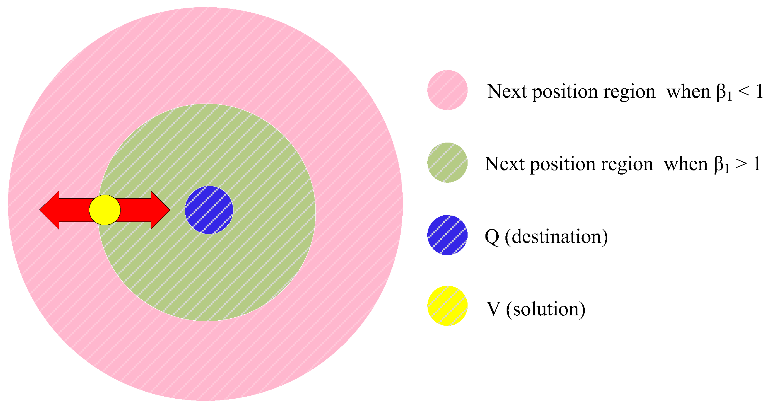
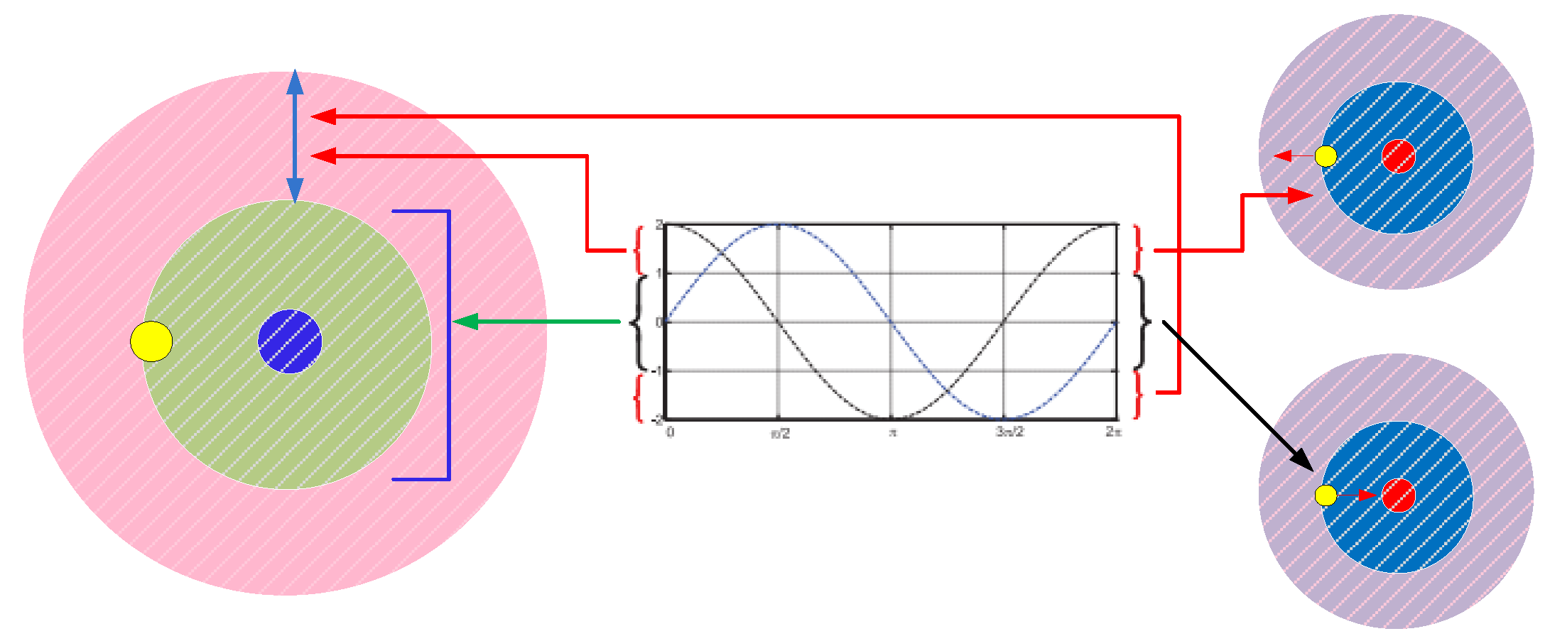
6. Sine-Cosine Algorithm (SCA)

The SCA initially creates a set of random population and allows them to move towards the best solution. In this algorithm, the optimization process contains two phases namely exploration and exploitation which lead to produce global (best) solution. The trigonometric functions namely sine sine and cosine functions are used to update the solutions in this algorithm. The position is updated as:
V p k + 1 = V p k + β 1 s i n ( β 2 ) | β 3 Q p k V p k | β 4 0.5
V p k + 1 = V p k + β 1 c o s ( β 2 ) | β 3 Q p k V p k | β 4 < 0.5
where V p k + 1 and V p k are old and updated positions of current solution at k-th iteration in p-th dimension. Q p k is the position of destination point in k-th dimension. The parameters β 2 , β 3 and β 4 are random numbers in the range of [ 0 , 1 ] . However, | . | represents the absolute value.
The distinctive features of sine and cosine functions of (36) and (37) are shown in Figure 6. By varying the value of β 1 , the amplitude of sine and cosine functions can be altered which results in finding a solution outside the space between their corresponding boundaries. Figure 7 shows exploration and exploitation of search space with sine and cosine wave-forms lying between [ 2 , 2 ] . In SCA algorithm, the balance exploration and exploitation can be achieved by changing β 1 using
β 1 = a k a T
where k is the current iteration, T is the total number of iterations and a is constant.

7. Test System

This section consists of two parts. In the first part, a test case is taken to explain model order reduction technique. In the second part, the design procedure of the FOPID controller for ROCIP is elaborated.

7.1. Improved Routh–Pade Approximation Method

Let the third-order SISO test system be given as
G 3 ( s ) = [ 3 , 4 ] s 2 + [ 25 , 26 ] s + [ 14 , 15 ] [ 7 , 8 ] s 3 + [ 54 , 55 ] s 2 + [ 90 , 91 ] s + [ 35 , 36 ] = A ( s ) B ( s )
The desired first-order model for (39) becomes
G 1 ( s ) = [ e 0 , e 0 + ] [ f 0 , f 0 + ] + [ f 1 , f 1 + ] s = E ( s ) F ( s )

7.1.1. Calculation of Denominator

The improved Routh Table (Table 1) for denominator of (39) obtained using (23) is given in Table 2.
The denominator of (40) is obtained from direct truncation of Table 2 which is given as
F ( s ) = 85.175 , 86.054 s + 35.06 , 35.94

7.1.2. Calculation of Numerator

The first interval TM and first interval MP of HOCIP, (39), are determined using (32) and (33), which are given as
[ λ 0 , λ 0 + ] = [ 0.389 , 0.428 ]
[ μ 1 , μ 1 + ] = [ 0.375 , 0.571 ]
The numerator polynomial of the desired first-order model, (40), can be obtained by matching first interval TM of HOCIP with first interval TM of ROCIP, such that
[ λ 0 , λ 0 + ] = [ λ 0 , λ 0 + ]
Using (34) and (42), the numerator polynomial is obtained as
E ( s ) = [ e 0 , e 0 + ] = [ 13.638 , 15.382 ]
Therefore, the desired first-order interval model, G 1 ( s ) , obtained from (41) and (45), is given as
G 1 ( s ) = [ 13.638 , 15.382 ] [ 85.175 , 86.054 ] s + [ 35.06 , 35.94 ]
Figure 8 represents the step response of interval transfer function (39) and its proposed model (46). It is clear from Figure 8 that the steady-state response of proposed model (46) and the system (39) are exactly identical, but when it comes to the transient state response there is a slight deviation between (39) and (46). Therefore, it can be concluded safely that the model preserves essential characteristics of the original system. This illustrates that proposed model (46) provides a good model of system (39).

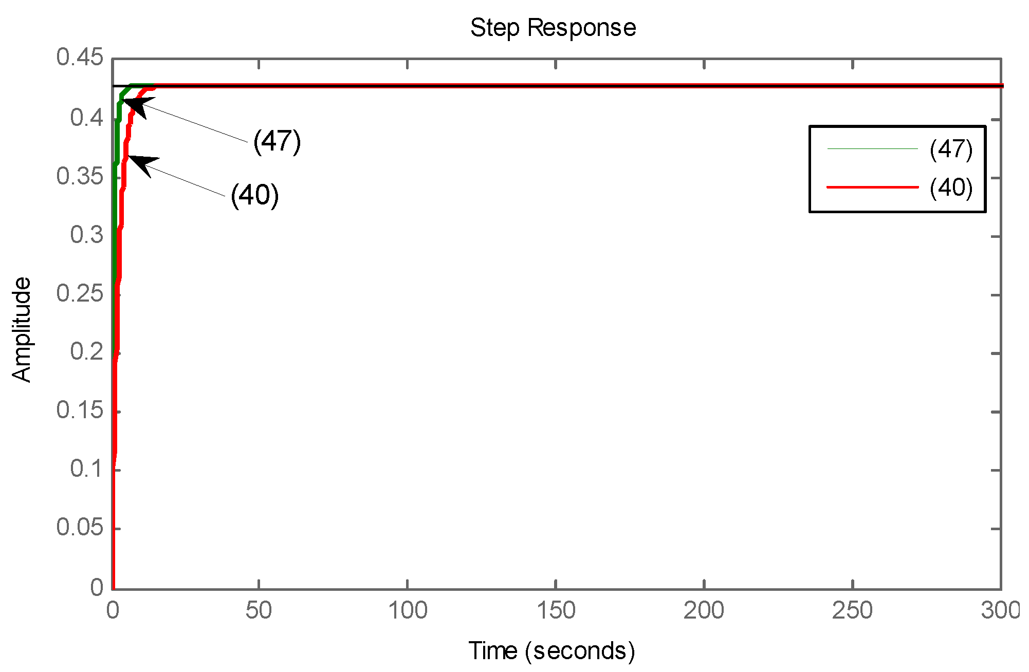
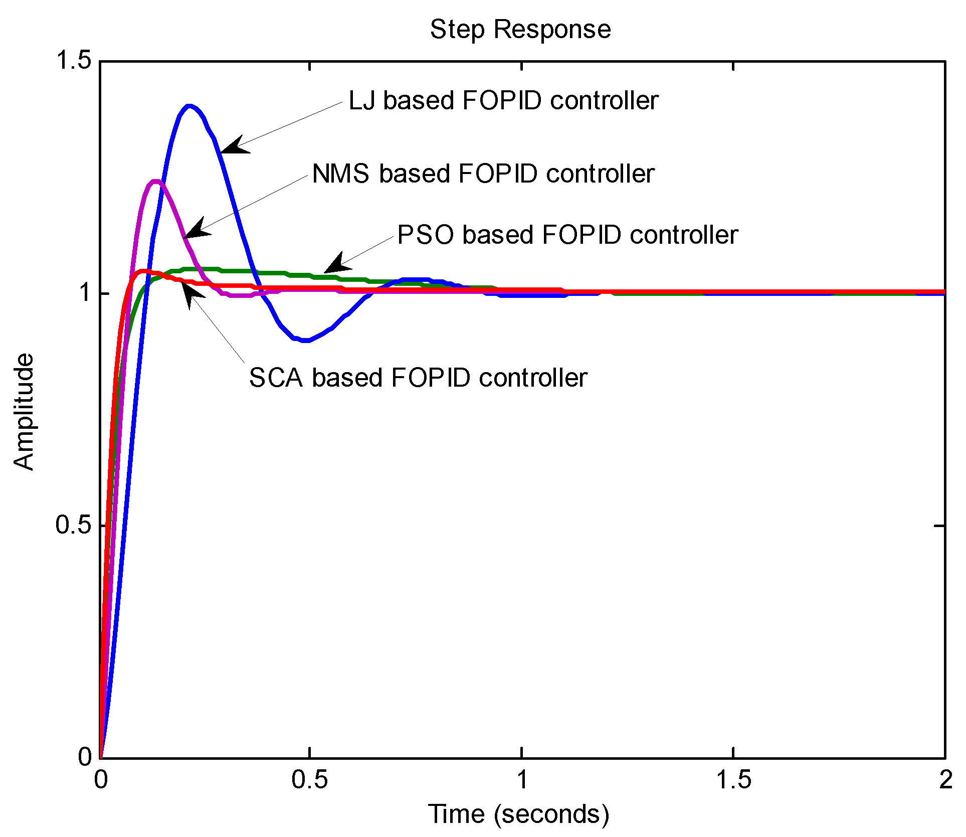
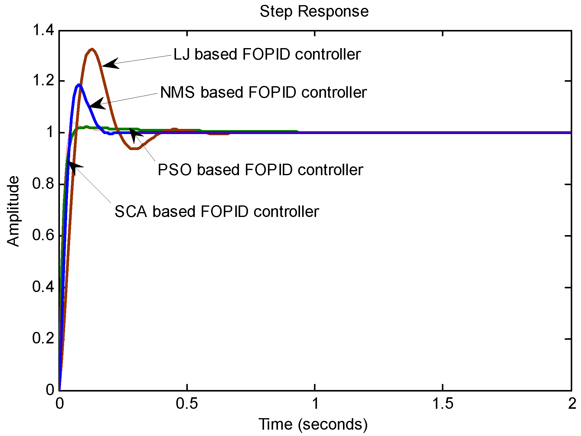
7.2. Design of FOPID Controller

An SCA-based FOPID controller is proposed for the first order interval system, (46), by considering the frequency domain specifications. In order to establish the efficacy of the SCA-based FOPID controller, other algorithms, namely particle swarm optimization (PSO) [61], Nelder–Mead simplex (NMS) [4] and Luus–Jaakola (LJ) [62,63] are also used to obtain the parameters of P I α D β controller. A total of 50 candidates are considered in whole population with 100 iterations for all algorithms. The key feature of the SCA algorithm [61,64,65,66] is that it is free from algorithm-specific parameters. The algorithm-specific parameters of all other algorithms are listed in Table 3.
In order to design the FOPID controller, different transfer functions are constructed as shown in Section 4.1. Using (16) and (18), the system transfer functions corresponding to maximum plots of gain and phase of the Bode envelope given as
G 1 b ( s ) = 15.382 85.175 s + 35.06
G 1 d ( s ) = 13.638 86.054 s + 35.06
The design criteria of the controlled system are considered as: gain crossover frequency ( ω g c ) = 50 rad/sec and phase margin ( ϕ p m ) = 85 deg.
Figure 9 represents the block diagram of ROCIP with an SCA-based FOPID controller. To obtain the desired specifications, (21) and (22) are solved using SCA. The optimal parameters ( K a , K b , K c , α and β ) of P I α D β controller obtained are
K a = 324.565 , K b = 658.081 , K c = 204.214 , α = 0.616 , β = 0.992
The FOPID controller for the specified design criteria is given as
C ( s ) = 324.565 + 658.081 s 0.616 + 204.214 s 0.992
The FOPID controllers for the above defined specifications obtained due to PSO, NMS and LJ are given as
C P S O ( s ) = 245.496 + 335.474 s 0.457 + 443.675 s 0.845
C N M S ( s ) = 832.765 + 147.164 s 0.329 + 379.852 s 0.693
C L J ( s ) = 473.359 + 259.876 s 0.478 + 156.952 s 0.573
Figure 10 presents the unit step response of closed-loop control system of Figure 4 and Figure 5 having ROCIP and HOCIP, respectively. From Figure 10, it is clearly observed that the designed FOPID controller C ( s ) using SCA for ROCIP, G 1 ( s ) , is also suited for HOCIP, G 3 ( s ) . This establishes the usefulness of proposed technique.
Figure 11 depicts the Bode plots of the open-loop controlled systems with FOPID controller. It is clear from the Figure 11 that frequency response of the SCA-based FOPID controller is also excellent for both ROCIP and HOCIP.
Figure 12 and Figure 13 plots the step responses of ROCIP and HOCIP with FOPID controllers obtained due to SCA, PSO, NMS and LJ. However, Figure 14 and Figure 15 are showing the Bode plots. It is clearly observed that the step responses of the closed-loop system with an SCA-based FOPID controller is better when compared to other optimization algorithms. The same is true for frequency response plotted in Figure 14 and Figure 15. This clearly established the supremacy of the SCA-based FOPID controller.
The comparative analysis is reported in Table 4. It is seen that the desired frequency domain specifications ( ω g c = 50 rad/sec and ϕ p m = 85 deg) of HOCIP are nearly fulfilled with an SCA assisted FOPID controller. The FOPID controllers designed using SCA, PSO, NMS, and LJ optimization techniques for HOCIP gives frequency domain specifications as ( ω g c = 87.32 rad/sec and ϕ p m = 54.7 deg), ( ω g c = 75.83 rad/sec and ϕ p m = 43.2 deg), ( ω g c = 58.57 rad/sec and ϕ p m = 28.3 deg) and ( ω g c = 31.54 rad/sec and ϕ p m = 33.7 deg), respectively. From these values, it is evident that the ω g c and ϕ p m obtained from the FOPID controllers designed using PSO, NMS and LJ are having larger deviations from the desired frequency domain specifications when compared to the FOPID controller based on SCA. This proves that the designed controller C ( s ) is robust and also best suited for both ROCIP and HOCIP to attain the desired specifications.

8. Conclusions

This article proposed a robust P I α D β controller based on sine-cosine algorithm (SCA) for high-order continuous interval plant (HOCIP) using a model order reduction technique. For controller design, HOCIP is initially diminished to reduced-order continuous interval plant (ROCIP) using the modified Routh–Pade approximation technique. The denominator polynomial of ROCIP is derived using modified Routh approximation which always guarantees the stability and the numerator polynomial is obtained by matching TMs and MPs that improve the transient and steady-state response of the ROCIP. Then, SCA algorithm is used to determine the five unknown parameters of P I α D β controller for ROCIP. The values of controller parameter are determined by minimizing two non-linear equations. For the design of P I α D β controller, gain crossover frequency ( ω g c ) and phase margin ( ϕ p m ) are considered as performance criteria. The simulation results demonstrate that the desired frequency domain specifications for both ROCIP and HOCIP are approximately fulfilled with the proposed SCA-based FOPID controller. Thus, it is established that proposed technique is an excellent alternative approach for the design of an FOPID controller using reduced-order modeling. The future line of work for the proposed technique lies in the design of a controller for multi-input-multi-output (MIMO) continuous and discrete interval systems.

Author Contributions

The paper was a collaborative effort among the authors. Conceptualization, methodology and simulation, J.K.B, N.P., T.V.; validation and formal analysis, J.K.B.; visualization and supervision, V.P.S. All authors have read and agreed to the published version of the manuscript.

Funding

The work reported herewith has been financially supported by SERB grant (Ref.: ECR/2017/000212).

Acknowledgments

SERB grant (ECR/2017/000212).

Conflicts of Interest

The authors declare no conflict of interest.

Abbreviations

The following abbreviations are used in this manuscript:
FOPIDfractional-order proportional-integral-derivative
PMphase margin
MPsMarkov parameters
TMstime moments
ROCIPreduced-order continuous interval plant
HOCIPhigh-order continuous interval plant
SCAsine-cosine algorithm
SISOsingle-input-single-output
MIMOmulti-input-multi-output
PIDproportional-integral-derivative
IOPIDinteger-order proportional-integral-derivative
AVRautomatic voltage regulator
MORmodel order reduction
ISEintegral-square-error
PSOparticle swarm optimization
RLRiemann–Liouville
GLGrunwald–Letnikov

References

  1. Cruz-Zavala, E.; Moreno, J.A. Homogeneous high order sliding mode design: A Lyapunov approach. Automatica 2017, 80, 232–238. [Google Scholar] [CrossRef]
  2. Almabrok, A.; Psarakis, M.; Dounis, A. Fast Tuning of the PID Controller in An HVAC System Using the Big Bang–Big Crunch Algorithm and FPGA Technology. Algorithms 2018, 11, 146. [Google Scholar] [CrossRef] [Green Version]
  3. Yang, G.; Yi, H.; Chai, C.; Huang, B.; Zhang, Y.; Chen, Z. Predictive current control of boost three-level and T-type inverters cascaded in wind power generation systems. Algorithms 2018, 11, 92. [Google Scholar] [CrossRef] [Green Version]
  4. Singh, S.; Singh, V.; Singh, V. Analytic hierarchy process based approximation of high-order continuous systems using TLBO algorithm. Int. J. Dyn. Control. 2019, 7, 53–60. [Google Scholar] [CrossRef]
  5. Nguyen, V.G.; Guo, X.; Zhang, C.; Tran, X.K. Parameter Estimation, Robust Controller Design and Performance Analysis for an Electric Power Steering System. Algorithms 2019, 12, 57. [Google Scholar] [CrossRef] [Green Version]
  6. Caponetto, R.; Machado, J.T.; Murgano, E.; Xibilia, M.G. Model Order Reduction: A Comparison between Integer and Non-Integer Order Systems Approaches. Entropy 2019, 21, 876. [Google Scholar] [CrossRef] [Green Version]
  7. Singh, V.P.; Chandra, D. Model reduction of discrete interval system using dominant poles retention and direct series expansion method. In Proceedings of the 2011 5th International Power Engineering and Optimization Conference, Shah Alam, Selangor, 6–7 June 2011; pp. 27–30. [Google Scholar]
  8. Zhang, S.; Yu, Y.; Wang, H. Mittag-Leffler stability of fractional-order Hopfield neural networks. Nonlinear Anal. Hybrid Syst. 2015, 16, 104–121. [Google Scholar] [CrossRef]
  9. Zhang, S.; Yu, Y.; Wang, Q. Stability analysis of fractional-order Hopfield neural networks with discontinuous activation functions. Neurocomputing 2016, 171, 1075–1084. [Google Scholar] [CrossRef]
  10. Monje, C.A.; Vinagre, B.M.; Feliu, V.; Chen, Y. Tuning and auto-tuning of fractional order controllers for industry applications. Control. Eng. Pract. 2008, 16, 798–812. [Google Scholar] [CrossRef] [Green Version]
  11. Liu, L.; Tian, S.; Xue, D.; Zhang, T.; Chen, Y. Continuous fractional-order zero phase error tracking control. ISA Trans. 2018, 75, 226–235. [Google Scholar] [CrossRef]
  12. Magin, R.; Ovadia, M. Modeling the cardiac tissue electrode interface using fractional calculus. J. Vib. Control. 2008, 14, 1431–1442. [Google Scholar] [CrossRef]
  13. Lassoued, A.; Boubaker, O. Dynamic analysis and circuit design of a novel hyperchaotic system with fractional-order terms. Complexity 2017, 2017. [Google Scholar] [CrossRef] [Green Version]
  14. Bingul, Z.; Karahan, O. Comparison of PID and FOPID controllers tuned by PSO and ABC algorithms for unstable and integrating systems with time delay. Optim. Control. Appl. Methods 2018, 39, 1431–1450. [Google Scholar] [CrossRef]
  15. Pitolli, F. A Collocation Method for the Numerical Solution of Nonlinear Fractional Dynamical Systems. Algorithms 2019, 12, 156. [Google Scholar] [CrossRef] [Green Version]
  16. Saleem, O.; Awan, F.G.; Mahmood-ul Hasan, K.; Ahmad, M. Self-adaptive fractional-order LQ-PID voltage controller for robust disturbance compensation in DC-DC buck converters. Int. J. Numer. Model. Electron. Netw. Devices Fields 2020, 33, e2718. [Google Scholar] [CrossRef]
  17. Alamdar Ravari, M.; Yaghoobi, M. Optimum design of fractional order pid controller using chaotic firefly algorithms for a control CSTR system. Asian J. Control. 2019, 21, 2245–2255. [Google Scholar] [CrossRef]
  18. Debbarma, S.; Saikia, L.C.; Sinha, N. Automatic generation control using two degree of freedom fractional order PID controller. Int. J. Electr. Power Energy Syst. 2014, 58, 120–129. [Google Scholar] [CrossRef]
  19. Podlubny, I. Fractional-order systems and fractional-order controllers. Inst. Exp. Phys. Slovak Acad. Sci. Kosice 1994, 12, 1–18. [Google Scholar]
  20. Aghababa, M.P. Optimal design of fractional-order PID controller for five bar linkage robot using a new particle swarm optimization algorithm. Soft Comput. 2016, 20, 4055–4067. [Google Scholar] [CrossRef]
  21. Mohsenipour, R.; Fathi Jegarkandi, M. Robust stability analysis of fractional-order interval systems with multiple time delays. Int. J. Robust Nonlinear Control. 2019, 29, 1823–1839. [Google Scholar] [CrossRef]
  22. Azarmi, R.; Tavakoli-Kakhki, M.; Fatehi, A.; Sedigh, A.K. Robustness analysis and design of fractional order Iλ Dμ controllers using the small gain theorem. Int. J. Control. 2020, 93, 449–461. [Google Scholar] [CrossRef]
  23. Liu, L.; Zhang, S. Robust fractional-order PID controller tuning based on Bode’s optimal loop shaping. Complexity 2018, 2018. [Google Scholar] [CrossRef]
  24. Saidi, B.; Amairi, M.; Najar, S.; Aoun, M. Bode shaping-based design methods of a fractional order PID controller for uncertain systems. Nonlinear Dyn. 2015, 80, 1817–1838. [Google Scholar] [CrossRef]
  25. Bhookya, J.; Jatoth, R.K. Optimal FOPID/PID controller parameters tuning for the AVR system based on sine–cosine-algorithm. Evol. Intell. 2019, 12, 725–733. [Google Scholar] [CrossRef]
  26. Mirjalili, S. SCA: A sine cosine algorithm for solving optimization problems. Knowl. Based Syst. 2016, 96, 120–133. [Google Scholar] [CrossRef]
  27. Khezri, R.; Oshnoei, A.; Tarafdar Hagh, M.; Muyeen, S. Coordination of heat pumps, electric vehicles and AGC for efficient LFC in a smart hybrid power system via SCA-based optimized FOPID controllers. Energies 2018, 11, 420. [Google Scholar] [CrossRef] [Green Version]
  28. Kumar, M.S.; Begum, G. Model order reduction of linear time interval system using stability equation method and a soft computing technique. Adv. Electr. Electron. Eng. 2016, 14, 153–161. [Google Scholar] [CrossRef]
  29. Singh, V.; Chauhan, D.P.S.; Singh, S.P.; Prakash, T. On time moments and Markov parameters of continuous interval systems. J. Circuits Syst. Comput. 2017, 26, 1750038. [Google Scholar] [CrossRef]
  30. Choudhary, A.K.; Nagar, S.K. Order reduction techniques via Routh approximation: A critical survey. IETE J. Res. 2019, 65, 365–379. [Google Scholar] [CrossRef]
  31. Potturu, S.R.; Prasad, R. Qualitative Analysis of Stable Reduced Order Models for Interval Systems Using Mixed Methods. IETE J. Res. 2018, 1–9. [Google Scholar] [CrossRef]
  32. Vijaya Anand, N.; Siva Kumar, M.; Srinivasa Rao, R. A novel reduced order modeling of interval system using soft computing optimization approach. Proc. Inst. Mech. Eng. Part J. Syst. Control. Eng. 2018, 232, 879–894. [Google Scholar] [CrossRef]
  33. Potturu, S.R.; Prasad, R. Model Order Reduction of LTI Interval Systems Using Differentiation Method Based on Kharitonov’s Theorem. IETE J. Res. 2019, 1–17. [Google Scholar] [CrossRef]
  34. Dulf, E.H. Simplified Fractional Order Controller Design Algorithm. Mathematics 2019, 7, 1166. [Google Scholar] [CrossRef] [Green Version]
  35. Kumar Deveerasetty, K.; Nagar, S. Model order reduction of interval systems using an arithmetic operation. Int. J. Syst. Sci. 2020, 51, 886–902. [Google Scholar] [CrossRef]
  36. Deveerasetty, K.K.; Zhou, Y.; Kamal, S.; Nagar, S.K. Computation of Impulse-Response Gramian for Interval Systems. IETE J. Res. 2019, 1–15. [Google Scholar] [CrossRef]
  37. Dewangan, P.; Singh, V.; Sinha, S. Improved Approximation for SISO and MIMO Continuous Interval Systems Ensuring Stability. Circuits Syst. Signal Process. 2020, 1–12. [Google Scholar] [CrossRef]
  38. Bia, P.; Mescia, L.; Caratelli, D. Fractional calculus-based modeling of electromagnetic field propagation in arbitrary biological tissue. Math. Probl. Eng. 2016, 2016. [Google Scholar] [CrossRef]
  39. Shen, X. Applications of Fractional Calculus In Chemical Engineering. Ph.D. Thesis, Université d’Ottawa/University of Ottawa, Ottawa, ON, Canada, 2018. [Google Scholar]
  40. Ortigueira, M.D.; Tenreiro Machado, J. Fractional calculus applications in signals and systems. Signal Process. 2006, 86, 2503–2504. [Google Scholar] [CrossRef]
  41. Douglas, J.F. Some applications of fractional calculus to polymer science. Adv. Chem. Phys. 1997, 102, 121–192. [Google Scholar]
  42. Oldham, K.B. Fractional differential equations in electrochemistry. Adv. Eng. Softw. 2010, 41, 9–12. [Google Scholar] [CrossRef]
  43. Bao, C.; Pu, Y.; Zhang, Y. Fractional-order deep backpropagation neural network. Comput. Intell. Neurosci. 2018, 2018, 7361628. [Google Scholar] [CrossRef] [PubMed]
  44. Kulish, V.V.; Lage, J.L. Application of fractional calculus to fluid mechanics. J. Fluids Eng. 2002, 124, 803–806. [Google Scholar] [CrossRef]
  45. Magin, R.L. Fractional Calculus in Bioengineering; Begell House: Redding, CA, USA, 2006; Volume 2. [Google Scholar]
  46. Soriano-Sánchez, A.G.; Rodríguez-Licea, M.A.; Pérez-Pinal, F.J.; Vázquez-López, J.A. Fractional-order approximation and synthesis of a PID controller for a buck converter. Energies 2020, 13, 629. [Google Scholar] [CrossRef] [Green Version]
  47. Petráš, I. Fractional-Order Nonlinear Systems: Modeling, Analysis and Simulation; Springer Science & Business Media: Berlin/Heidelberg, Germany, 2011. [Google Scholar]
  48. Gu, D.W.; Petkov, P.; Konstantinov, M.M. Robust control design with MATLAB®; Springer Science & Business Media: Berlin/Heidelberg, Germany, 2005. [Google Scholar]
  49. Tarasov, V.E.; Tarasova, S.S. Fractional derivatives and integrals: What are they needed for? Mathematics 2020, 8, 164. [Google Scholar] [CrossRef] [Green Version]
  50. Tejado, I.; Vinagre, B.M.; Traver, J.E.; Prieto-Arranz, J.; Nuevo-Gallardo, C. Back to basics: Meaning of the parameters of fractional order PID controllers. Mathematics 2019, 7, 530. [Google Scholar] [CrossRef] [Green Version]
  51. Khubalkar, S.; Chopade, A.; Junghare, A.; Aware, M.; Das, S. Design and realization of stand-alone digital fractional order PID controller for Buck converter fed DC motor. Circuits Syst. Signal Process. 2016, 35, 2189–2211. [Google Scholar] [CrossRef]
  52. Sondhi, S.; Hote, Y.V. Fractional order controller and its applications: A review. Proc. AsiaMIC 2012. [Google Scholar] [CrossRef]
  53. Podlubny, I. Fractional-order systems and PI/sup/spl lambda//D/sup/spl mu//-controllers. IEEE Trans. Autom. Control. 1999, 44, 208–214. [Google Scholar] [CrossRef]
  54. Nise, N.S. Control Systems Engineering; John Wiley & Sons: Hoboken, NJ, USA, 2020. [Google Scholar]
  55. Ortigueira, M.D.; Trujillo, J.J.; Martynyuk, V.I.; Coito, F.J. A generalized power series and its application in the inversion of transfer functions. Signal Process. 2015, 107, 238–245. [Google Scholar] [CrossRef]
  56. Dolgin, Y. Author’s reply [to comments on’On Routh-Pade model reduction of interval systems’]. IEEE Trans. Autom. Control. 2005, 50, 274–275. [Google Scholar] [CrossRef]
  57. Vinagre, B.M.; Monje, C.A.; Calderón, A.J.; Suárez, J.I. Fractional PID controllers for industry application. A brief introduction. J. Vib. Control. 2007, 13, 1419–1429. [Google Scholar] [CrossRef]
  58. Monje, C.A.; Calderon, A.J.; Vinagre, B.M.; Chen, Y.; Feliu, V. On fractional PI λ controllers: Some tuning rules for robustness to plant uncertainties. Nonlinear Dyn. 2004, 38, 369–381. [Google Scholar] [CrossRef]
  59. Yeroglu, C.; Tan, N. Note on fractional-order proportional–integral–differential controller design. IET Control. Theory Appl. 2011, 5, 1978–1989. [Google Scholar] [CrossRef]
  60. Pal, J. System reduction by a mixed method. IEEE Trans. Autom. Control. 1980, 25, 973–976. [Google Scholar] [CrossRef]
  61. Singh, V. Sine cosine algorithm based reduction of higher order continuous systems. In Proceedings of the 2017 International Conference on Intelligent Sustainable Systems (ICISS), Palladam, India, 7–8 December 2017; pp. 649–653. [Google Scholar]
  62. Srivastava, S.; Singh, V.; Singh, S.; Dohare, R.; Kumar, S. Luus-Jaakola based PID controller tuning for double tank system. Int. J. Adv. Technol. Eng. Explor. 2016, 3, 199. [Google Scholar] [CrossRef]
  63. Singh, V.P.; Chandra, D.; Rastogi, R. Luus jaakola algorithm based order reduction of discrete interval systems. Pratibha Int. J. Sci. Spirit. Bus. Technol. IJSSBT 2012, 1, 1–8. [Google Scholar]
  64. Prakash, T.; Singh, S.; Singh, V. Analytic hierarchy process-based model reduction of higher order continuous systems using sine cosine algorithm. Int. J. Syst. Control. Commun. 2020, 11, 52–67. [Google Scholar] [CrossRef]
  65. Mehra, S.; Monga, H.; Singh, V.; Kumar, R. Application of SCA for Level Control of Three-Tank System. In Proceedings of the 2020 International Conference on Computation, Automation and Knowledge Management (ICCAKM), Dubai, UAE, 9–10 January 2020; pp. 220–224. [Google Scholar]
  66. Thakur, A.; Monga, H.; Singh, V.; Kumar, R.; Mathur, A. Sine Cosine Algorithm Assisted Tuning of PID Controller for DC Servo-Motor. In Proceedings of the 2020 International Conference on Computation, Automation and Knowledge Management (ICCAKM), Dubai, UAE, 9–10 January 2020; pp. 230–233. [Google Scholar]
Figure 1. Block diagram of closed loop control system.
Algorithms 13 00317 g001
Figure 2. Closed loop system of HOCIP.
Algorithms 13 00317 g002
Figure 3. Closed loop system of ROCIP.
Algorithms 13 00317 g003
Figure 4. Closed loop ROCIP with FOPID controller.
Algorithms 13 00317 g004
Figure 5. Closed loop HOCIP with FOPID controller.
Algorithms 13 00317 g005
Figure 6. The result of the sine and cosine functions in (36) and (37) for the next stage [26].
Algorithms 13 00317 g006
Figure 7. Sine and cosine functions within the range of [−2, 2] allow a way to move around (inside the space among them) or beyond (outside the space among them) the target [26].
Algorithms 13 00317 g007
Figure 8. Step response of system G 3 ( s ) and model G 1 ( s ) .
Algorithms 13 00317 g008
Figure 9. ROCIP with an SCA-based FOPID controller.
Algorithms 13 00317 g009
Figure 10. Unit step response of controlled ROCIP and HOCIP.
Algorithms 13 00317 g010
Figure 11. Bode plots of controlled ROCIP and HOCIP with an FOPID controller.
Algorithms 13 00317 g011
Figure 12. Step response of controlled ROCIP with the FOPID controller.
Algorithms 13 00317 g012
Figure 13. Step response of controlled HOCIP with the FOPID controller.
Algorithms 13 00317 g013
Figure 14. Bode response of controlled ROCIP with FOPID controller
Algorithms 13 00317 g014
Figure 15. Bode response of controlled HOCIP with the FOPID controller.
Algorithms 13 00317 g015
Table 1. Modified Routh array.
T 1 , 1 = B n T 1 , 2 = B n 2 T 1 , 3 = B n 4
T 2 , 1 = B n 1 T 2 , 2 = B n 3
T 3 , 1 T 3 , 2
T n , 1 T n , 2
T n + 1 , 1
Table 2. Routh array for denominator polynomial of (39).
s 3 7 , 8 90 , 91
s 2 54 , 55 35.06 , 35.94
s 1 85.175 , 86.054
s 0 35.06 , 35.94
Table 3. Algorithm-specific parameters for different algorithms.
AlgorithmsParametersValues
PSOCognitive parameter, c 1
Social parameter, c 2
Inertia weight, w
2
2
0.5
NMSRefection coefficient, α
Contraction coefficient, β
Expansion coefficient, γ
Shrinking coefficient, δ
1
1 / 2
2
1 / 2
LJContraction factor, γ 0.95
SCANo parameter
Table 4. Controller parameters and specifications for different algorithms.
Algorithms ϕ p c (deg) ω g c (rad/sec) K a K b K c α β
SCA 87.32 54.7 324.565 658.081 204.214 0.616 0.992
PSO 75.83 43.2 245.496 335.474 443.675 0.457 0.845
NMS 58.57 28.3 832.765 147.164 379.852 0.329 0.693
LJ 31.54 33.7 473.359 259.876 156.952 478 0.573
Publisher’s Note: MDPI stays neutral with regard to jurisdictional claims in published maps and institutional affiliations.

