Article

Groundwater Prediction Using Machine-Learning Tools

1
Department of Computer Science, University of the Western Cape, Cape Town 7535, South Africa
2
Department of Science and Mathematics, University-Central Texas, Killeen, TX 76549, USA
3
Department of Physics and Astronomy, University of the Western Cape, Cape Town 7535, South Africa
*
Author to whom correspondence should be addressed.
Algorithms 2020, 13(11), 300; https://doi.org/10.3390/a13110300
Submission received: 6 October 2020 / Revised: 26 October 2020 / Accepted: 2 November 2020 / Published: 17 November 2020
(This article belongs to the Special Issue Interpretability, Accountability and Robustness in Machine Learning)

Abstract

:
Predicting groundwater availability is important to water sustainability and drought mitigation. Machine-learning tools have the potential to improve groundwater prediction, thus enabling resource planners to: (1) anticipate water quality in unsampled areas or depth zones; (2) design targeted monitoring programs; (3) inform groundwater protection strategies; and (4) evaluate the sustainability of groundwater sources of drinking water. This paper proposes a machine-learning approach to groundwater prediction with the following characteristics: (i) the use of a regression-based approach to predict full groundwater images based on sequences of monthly groundwater maps; (ii) strategic automatic feature selection (both local and global features) using extreme gradient boosting; and (iii) the use of a multiplicity of machine-learning techniques (extreme gradient boosting, multivariate linear regression, random forests, multilayer perceptron and support vector regression). Of these techniques, support vector regression consistently performed best in terms of minimizing root mean square error and mean absolute error. Furthermore, including a global feature obtained from a Gaussian Mixture Model produced models with lower error than the best which could be obtained with local geographical features.

1. Introduction

In many countries, groundwater is one of the key natural resources that supplies a large portion of the water used by a nation. Besides its use in households and businesses, some other groundwater consumers include: (i) rural households and public water supplies that depend on wells and groundwater; (ii) farmers who use groundwater to irrigate crops and water their animals; and (iii) commercial businesses and industries that depend on groundwater for their processes and operations. Furthermore, the importance of groundwater can be revealed in its usage in supplying springs, water in ponds, marshlands, swamps, streams, rivers and bays. However, despite its unequivocal importance, groundwater levels in aquifer systems are often not constant and depend on recharge from infiltration of precipitation.
Several major acts and regulations such as the South African national water Act [1] and the 4th World Water Forum [2] recognize water as a basic human need, which is a major contributor to social development since it helps to alleviate poverty [1]. Hence, there is a growing interest towards the use of groundwater to help alleviate this crisis [2]. Groundwater is a vital freshwater resource which provides around 50% of the available drinking water according to UNESCO [3]. Also, sectors like agriculture, and industry greatly depend on groundwater for their operations due to its widespread availability and the fact that it is not easy polluted [3,4]. Therefore, in 2015 the United Nations have reaffirmed their commitment regarding the human right to safe drinking water and sanitation by identifying it as one of the 17 Sustainable Development Goals to be pursued by 2030 [5].
Predicting groundwater availability is important to water sustainability and drought mitigation. It can provide useful insights based on real data of what happened when the flow of streams and rivers declined and/or when water supply issues developed into a drought. Machine-learning tools technologies have the potential to drive groundwater knowledge discovery and management by assisting in the prediction of groundwater availability. This can be done by enabling the collection of massive water datasets, storing these datasets into databases and processing these datasets to get useful insights which can be used by water resource managers to: (1) anticipate water quality in unsampled areas or depth zones; (2) design targeted monitoring programs; (3) inform groundwater protection strategies; and (4) evaluate the sustainability of groundwater sources of drinking water.
This paper uses a regression-based approach to predict full groundwater images based on sequences of monthly groundwater maps of the southern part of the African continent using the Gravity Recovery and Climate Experiment (GRACE) dataset [6]. Five machine-learning techniques are implemented on the GRACE dataset and compared to predict pixels in future frames of the dataset. These are extreme gradient boosting (XGB), multivariate linear regression (MLR), random forest (RF), multilayer perceptron (MLP) and support vector regression (SVR). The prediction is guided by: (i) performing feature selection based on the XGB feature importance bar on the previous lags (pixels); and (ii) investigating the effect of adding other features such as the temporal features, position indices, and global features obtained by Gaussian mixture models (GMMs) fitted to peak areas on each image.
This paper is organized as follows: Section 2 provides a background on water prediction, citing relevant literature in the field; Section 3 describes the algorithms used in this work; Section 4 discusses the methodology used for ground water prediction; Section 5 provides and discusses the results obtained; and Section 6 furnishes the conclusions.

2. Background on Groundwater Prediction

With the increase in population size coupled with urban expansion, water demand has dramatically increased, which has led to the over-exploitation of groundwater in many countries around the world [7,8]. This highlights the importance of groundwater forecasting. Accurate prediction of groundwater can help government officials determine the best approach to manage groundwater effectively [9]. The main tools for groundwater prediction are based on physical models and data-driven models [10]. Physical models require a large amount of detailed hydrological data, which suffers from a lack of accuracy during its collection and pre-processing [9]. Therefore, data-driven models tend to be more appealing, since they require less data and are more reliable [3,11].
Statistical models like multivariate linear regression (MLR), and various time series models such as autoregressive moving average (ARMA), autoregressive integrated moving average (ARIMA) and seasonal ARIMA (SARIMA), have been used to investigate patterns between the input and the output of groundwater data to make future predictions. The following studies have investigated: MLR for groundwater prediction [12,13,14]; and time series models for groundwater prediction [12,15,16,17]. Both techniques are considered to be linear fitting models [11]. Time series models have the advantage of accounting for the correlations that arise between data points [18]. In general, however, linear fitting is not ideal in describing the nonlinear behavior of groundwater. Hence, recent research has made use of MLR models more for comparative purposes [11].
In addition to these techniques, a range of machine-learning techniques have been applied to the problem, including MLP in [12,19,20,21,22,23], SVR in [19,24] and recently RFs in [25,26]. The use of XGB is rare in the scheme of groundwater prediction, and is found in only a few studies such as [27,28].
The above studies can be broadly divided into those that predict the groundwater level (GWL) and those that estimate the terrestrial water storage ( Δ TWS ). GWL provides an idea of the groundwater level, whereas Δ TWS provides an idea about the volume of the groundwater. The GRACE database gives geographical Δ TWS levels monthly [6]. The significance of GRACE in hydrology is that it can provide an understanding of groundwater storage conditions and trends [29]. GRACE has been used as a predictor to help in the estimation of the GWL in [29,30].
In the literature, there are two main approaches to the problem of sequential image prediction. The first type involves taking a sequence of images as an input to predict future frames using deep learning techniques such as Convolutional Long-Short-Term-Memory (ConvLSTM). Usually, the images used for this type of prediction are separated by relatively short time intervals e.g., 6–10 min [31,32,33,34,35,36,37]. This approach normally does not involve any feature selection approach, since deep learning related techniques are known for their feature selection and reduction properties. However there are several concerns when using deep learning models: they depend heavily on a large quantity of high quality data to produce an effective model; they are very costly to train and use, in terms of time and resources; deep learning models are often viewed as black boxes [38] which means that it is very difficult to unpack and understand the automated feature selection process that eventually takes place and the predictions that arise from any given deep-learning-based model.
This leads us to the second approach in which machine-learning techniques can be used for single-output regressing problems. For GRACE Δ TWS image reconstruction, the authors in [27] used both XGB and RFs to acquire the importance of 20 features. It was shown that the precipitation of the two months prior to prediction is the most important variable for estimating the TWS dynamics. In [28], authors manually selected 11 hydrological predictors including the total precipitation and snow cover to predict Δ TWS . As for the idea of using previous pixels to predict current pixels has not been investigated enough in the literature. The authors in [39] made a comparison between Support Vector Machines (SVMs) and RF in predicting the present grid-based rainfall up to 3 h ahead, where the input involved the antecedent radar-derived rainfall. The authors in [40], used ANNs to predict full water vapor images every 30 min, where they included information from two previous images.

3. Techniques Used

In the following section we describe the tools and the technologies that has been used during the study. A total of five machine-learning techniques were used in this study for image prediction: (a) MLR; (b) MLP; (c) RF; (d) XGB; and (e) SVR.
Aside from the task of prediction, XGB was also used as a feature extraction and selection tool. As for feature engineering we used Gaussian Mixture Models (GMMs) to capture global features—mean and variance—of past images. For evaluation of the trained models, we used the RMSE and the MAE as evaluation metrics. All of the above-mentioned tools were implemented using the scikit-learn library [41] in the Anaconda python distribution (version 2020.07) with their default hyper-parameter settings.
Section 3.1, Section 3.2, Section 3.3, Section 3.4, Section 3.5 and Section 3.6 describe each of the five machine-learning techniques listed above. Section 3.7 describes the metrics used to evaluate the trained models.

3.1. Multivariate Linear Regression

The level of correlation between the predictors and the output variables are usually estimated by regression models to determine their relationship form [42]. In linear regression, the mean square error is used to fit the models and to assess the performance of the trained models on the testing set [42,43]. In general, MLR is used to discover the hyperplane that best fits all individual data points [42]. For simplicity, in the following sections, MLR will be abbreviated as LR.

3.2. Multilayer Perceptron

MLPs are a type of artificial neural networks, which is a class of models inspired by the biological nervous system of the human brain. They can emulate complex functions like decision making, and pattern generation [44]. Like the human brain, MLPs also consist of a set of processing units called ‘neurons’, which are connected to each other. Each neuron is a multi-input and single-output nonlinear element [45]. Neurons mostly operate in parallel, and are arranged in multiple layers which include an input layer into which the data are fed; hidden layer where the learning takes place; and an output layer [44]. MLPs can detect complex nonlinear relationships through a learning process that involves the adjustment of the weighted connections that exists between the neurons. This gives MLPs the ability to perform two important functions: pattern classification and nonlinear adaptive filtering [46].

3.3. Random Forest

RF uses an ensemble of classification and regression trees. Each tree is built using a different bootstrap sample (with replacement) from the original data [47]. Compared to traditional trees, RF adds a randomness layer to bagging, since in traditional trees each node is split using the best split among all variables [48]. As for RF, only a random subset of the variables is used when splitting a node during the construction of a tree [47,48]. As a result of the random constructions, RF provides robustness to overfitting as compared to some other techniques [48,49].

3.4. eXtreme Gradient Boosting

Like RF, XGB is an ensemble learning technique. XGB relies on gradient boosting to form a combined prediction. In XGB, the predictors in a tree are built in a sequential manner, and are trained on the residuals of the previous learners, so that errors are reduced step by step [27].
In the scikit-learn implementation in XGB, the plot.importance command can be used to determine feature importance for the features in trained predictive model [50]. The plot.importance command computes for each separate feature the sum of estimated improvements in squared error risk for all decision nodes employing that feature, averaged over all trees used in the model. The averaging greatly reduces the masking effect which occurs when variables are correlated [51].

3.5. Support Vector Machine and Support Vector Regression

SVM is a powerful machine-learning technique that has the capability to perform structural risk minimization (SRM), which enables it to avoid overfitting by minimizing the bound on the generalization error [52]. SVMs may be extended to apply to estimation and regression problems: this extension is known as support vector regression (SVR) [53]. SVR maps the input data into a higher-dimensional feature space via nonlinear kernel functions [54]. The objective is to choose a vector of regression coefficients with a small norm, while minimizing the sum of the distances between the data points and the regression hyperplane in the higher-dimensional space [55].

3.6. Gaussian Mixture Models

Gaussian mixture models (GMMs) may be used for clustering [56] or as parametric models of the probability distribution of continuous features [57]. The user specifies the number of Gaussians in the model, and the means and covariances of the Gaussians are automatically computed using an expectation maximization (EM) algorithm [58].

3.7. Performance Metrics

The accuracies of the above machine-learning models are evaluated using the root mean square error (RMSE) and the mean absolute error (MAE). Both metrics are commonly used to measure the forecasting accuracy [59]. RMSE is more sensitive to outliers and is more appropriate for Gaussian-distributed errors, while MAE weights all errors equally [60]. The RMSE and MAE are computed as follows:
RMSE = 1 n i = 1 n ( y i o b s y i p r e ) 2
MAE = 1 n i = 1 n | y i o b s y i p r e |
where y i o b s and y i p r e refer to the observed and predicted value of the i t h output, respectively.

4. Groundwater Prediction Methodology

Following the flowchart in Figure 1, we start by discussing the data set, followed by the pre-processing of the images and the preparation of the data set. Then we speak about the feature selection that was done using XGB, and feature engineering using GMM. Finally, we end up with the experiment. Our end goal is to predict groundwater on a pixel level to end up with a full image using a sequence of images as an input.

4.1. Monthly Groundwater Data Set

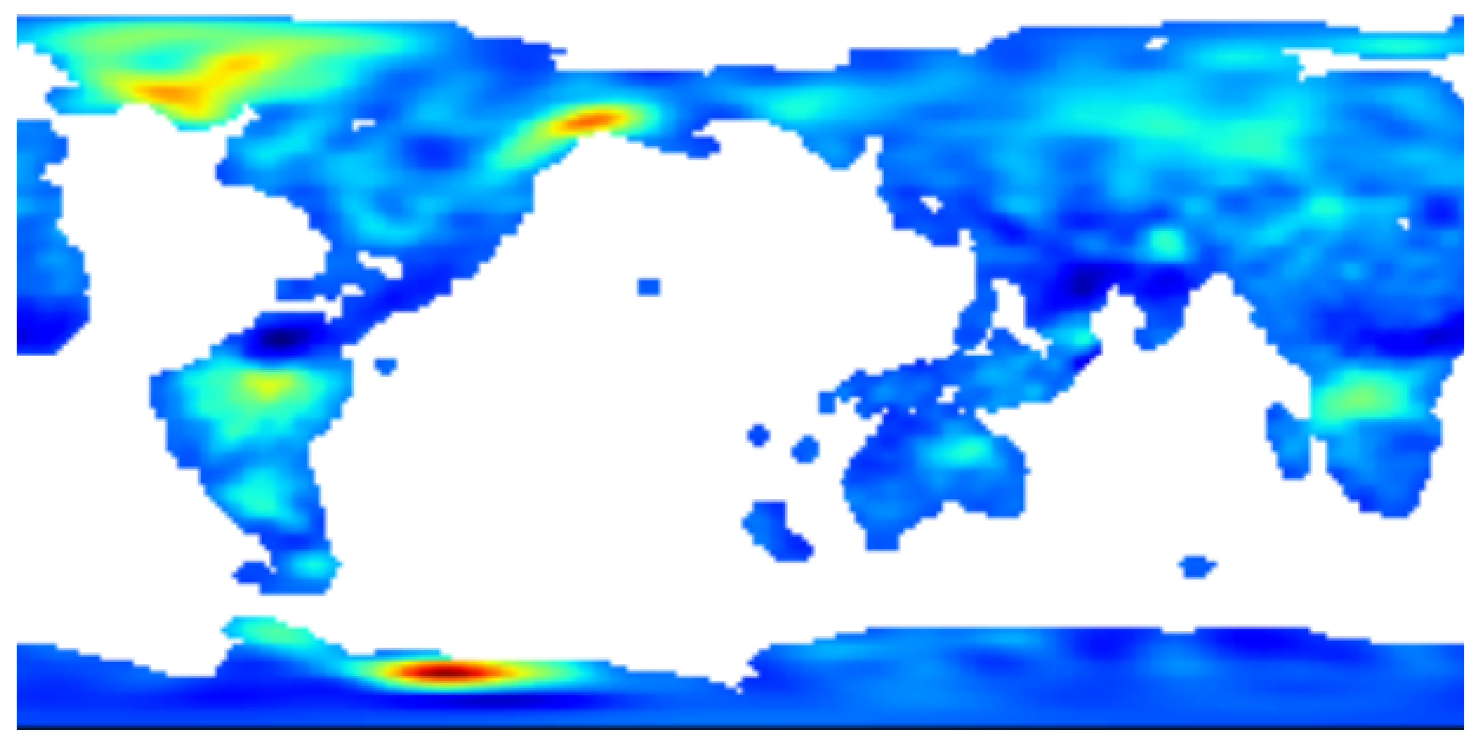
The dataset used in this study consists of 174 monthly groundwater satellite images between March 2002 and May 2019. Each image has a size of 360 × 180 pixels, and provides a color-coded representation of the Δ TWS of the earth’s land surface. A sample image from the dataset is provided in Figure 2. The images were originally obtained as part of the GRACE survey conducted by the U.S. National Aeronautical and Space Administration (NASA). The actual data was obtained from the Physical Oceanography Distributed Active Archive Center (PO. DAAC) website [6].
Using this dataset posed some serious challenges. Several monthly images in the dataset were missing. Neglecting these months would disrupt the periodicity/seasonality in the data, which is a key aspect of the data. Further reducing the dataset was not feasible, since the number of images is already on the small side for machine-learning applications. Finding better methods for dealing with missing images is an ongoing research topic.

4.2. Image Pre-Processing

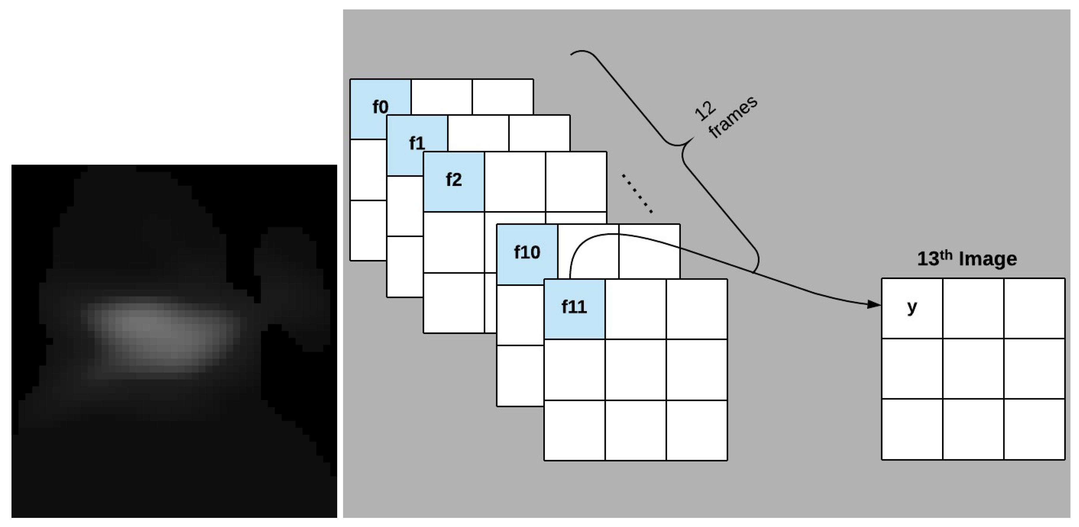
Predicting a full color image at the pixel level would be computationally expensive, since the full image consists of R,G,B values for 360 × 180 × 3 pixels. Hence, to reduce the computational cost, we transformed the images into grayscale, and cropped the images to focus on the southern area of the African continent with a size of 47 × 51 . An image of the pre-processed data is shown in Figure 3 (left).
The dataset provided from PO.DAAC had missing months. We imputed the data for the missing months by replicating the previous months’ images. Out of the 174 frames, we deleted the first two frames because of a gap of about 100 days between the 2nd and the 3rd image in the data. This left 172 images, and after image imputation we ended up with a dataset of 190 images. Altogether 18 images were imputed, which amount to about 10% of the original 172 images. We then applied a sliding window to form 161 sequences of 12 consecutive images. The first 149 sequences were used for training, and the rest for testing. We did not use any of the imputed images as labels for the models to train on.

4.3. Feature Selection

Since the dataset in this research is small, it was particularly important to choose a set of features of limited size (to avoid overfitting) but which still captures essential information that can be used for prediction. In our model we used both local and global spatiotemporal features, and additionally performed a rescaling, as described in the following subsections.

4.3.1. Same-Pixel Features

Our first set of candidate features for prediction of an image pixel consists of the same pixel location for the 12 previous months. A similar choice has been made in previous studies [39,40,61]. To select the most important of these 12 features, a sliding window technique is used, as shown in Figure 3 (right): the same pixels within a prior 12-month window were used to predict the corresponding pixel in the 13th month.
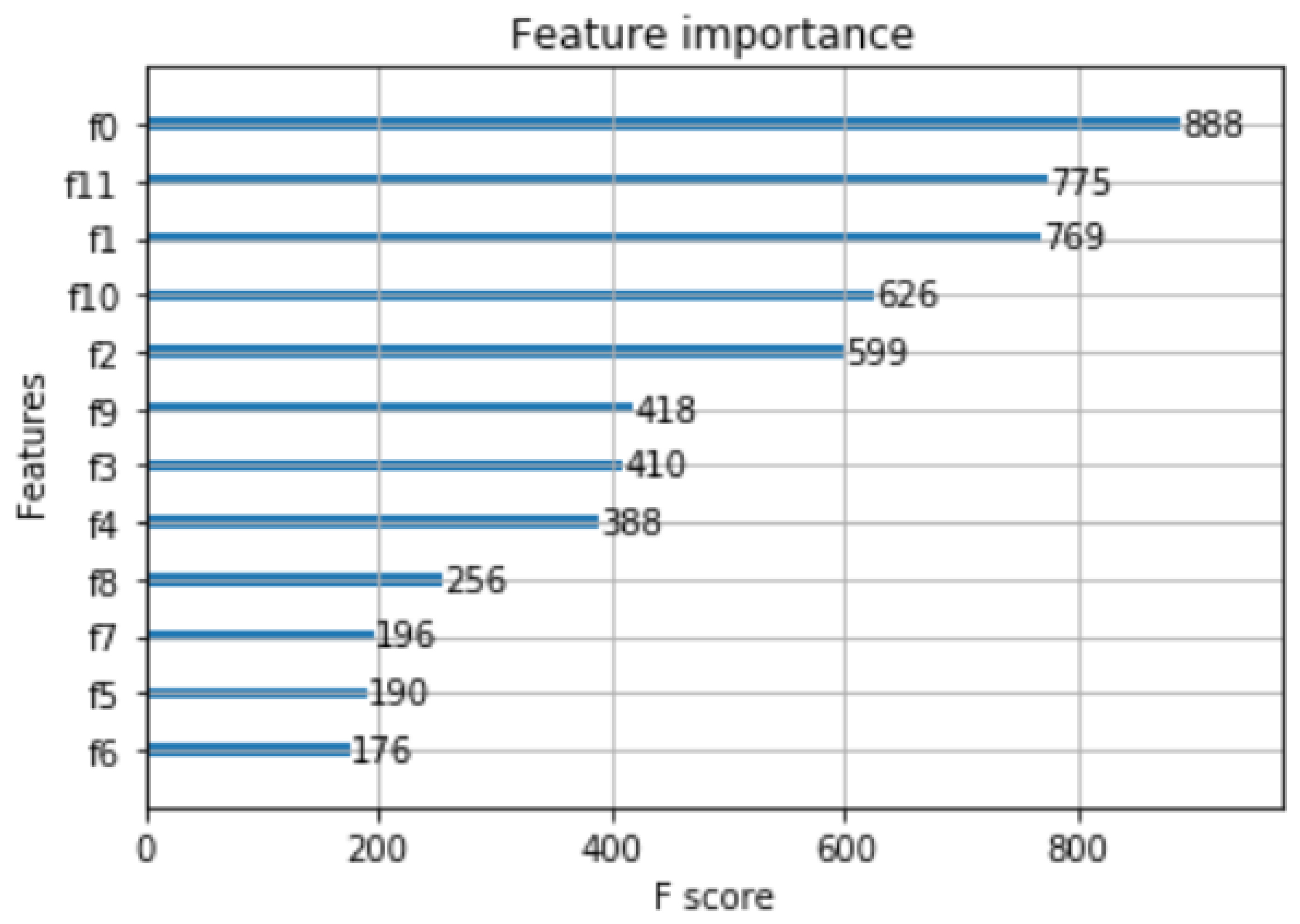
To evaluate the relative importance of these features, XGB with the gain metric was applied to the training set. Figure 4 shows the results. In the figure, f(0) stands for the same month in the previous year while f(11) stands for the previous month. The graph shows that f(0), f(11), and f(1) (12, 1, and 11 months previous, respectively) have the greatest importance. This finding agrees with [62,63], which also used the previous and 12-month prior pixels to predict corresponding points in current month.
Based on our results, we created seven different feature sets labelled ag as follows:
  • a = f(0, 11)
  • b = f(0, 11, 1)
  • c = f(0, 11, 1, 10)
  • d = f(0, 11, 1, 10, 2)
  • e = f(0, 11, 1, 10, 2, 9)
  • f = f(0, 11, 1, 10, 2, 9, 3)
  • g = f(0, 11, 1, 10, 2, 9, 3, 8, 4)

4.3.2. Other Local Spatiotemporal Features, and Rescaling

Because of the geographical and seasonal nature of groundwater levels, the following spatiotemporal features were also deemed to be significant and were used:
  • Pixel’s x , y coordinate;
  • Time stamp ( 0 , , 11 ) (0 = January, …11 = December)
Since most of the pixel values are low and high values were relatively infrequent, the pixel values were replaced by their square roots to regularize the scale. The square root transformation was similarly applied to inputs in [64], and to outputs in [65,66].

4.3.3. Global Feature Generation Using Gaussian Mixture Models

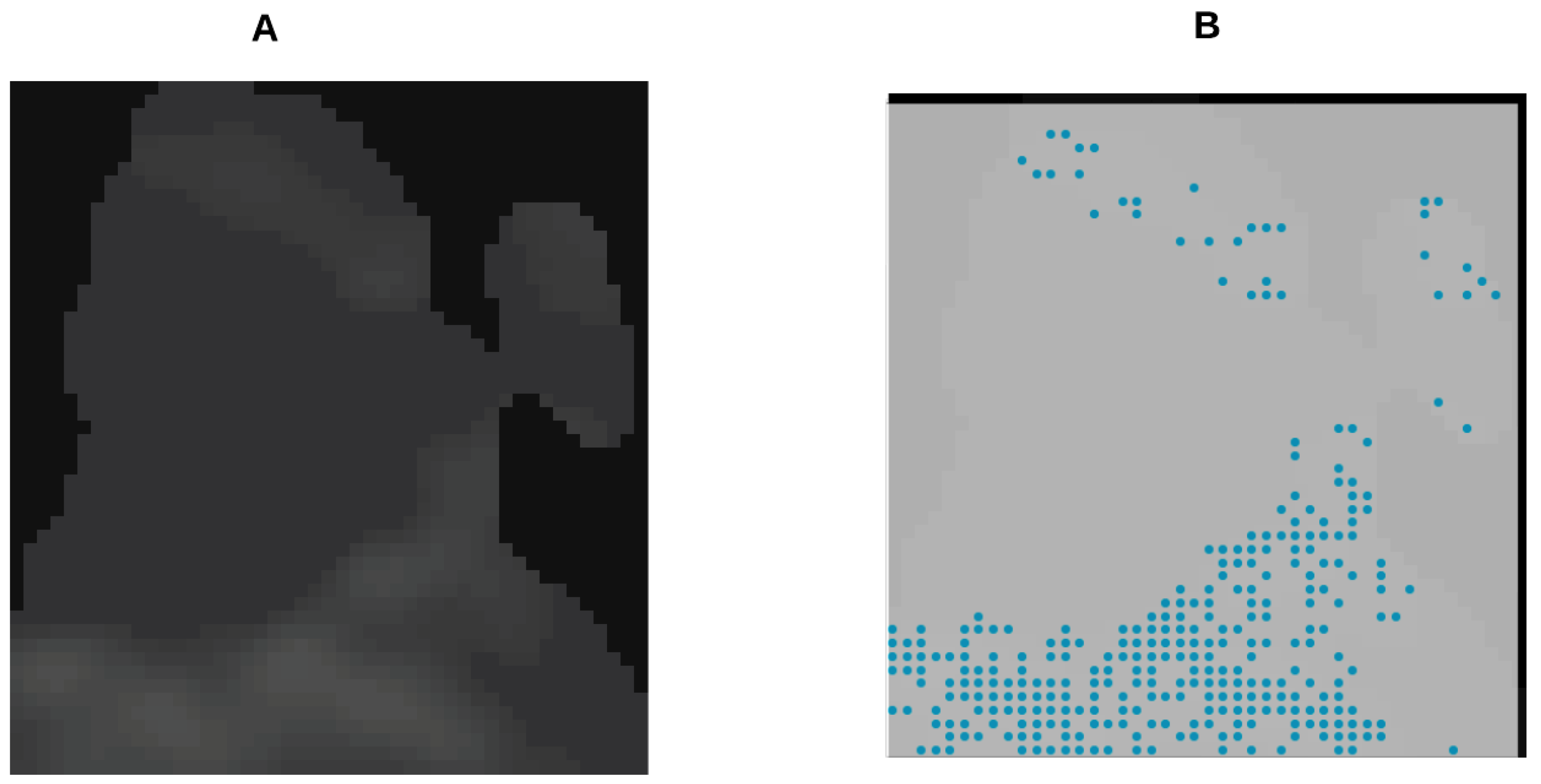
In this subsection we describe how we used Gaussian mixture models (GMMs) to generate global features. This idea came from observing that regions of high groundwater level seemed to form shapes that could be described as Gaussian distributions, which propagated from image to image. The means and the covariances of these Gaussian-shaped features can be used as global features that describe the motion of high regions from image to image. To apply GMM to an image, we converted the image to a set of pixel locations by randomly selecting pixels with selection probability proportional to the pixel’s scaled intensity (see Figure 5). These pixel locations were fed to the GMM algorithm which returned means, covariance matrices, and weights of Gaussian clusters. In this study, we set up the algorithm to have only one cluster. The pixel located at the cluster mean and the two eigenvalues of the covariance matrix were used as global features.
We applied GMM to image 10 (two months previous), and image 11 (one month previous), yielding a total of 8 global features. As described above, our application of GMM involved a randomization when choosing pixel locations. To account for this randomness, when evaluating models that used GMM features we created 100 different models using different randomization. From those 100 results we took the per-pixel averages to get a single model, and took the RMSE and MAE for this model to obtain accuracy estimates.

5. Performance Results and Discussion

5.1. Performance Results

Table 1, Table 2, Table 3 and Table 4 show performance accuracies for models trained using different features. Table 1 uses only same-pixel data from previous months; Table 2 adds the features (i,j), which stands for the pixels position in a 2D array; Table 3, adds the time stamp (denoted by t); Table 4, additionally applies the square root transformation (denoted by s) to the pixel values. The code together with image data is available on GitHub at https://github.com/EslamHussein55/Groundwater-Pixel-Prediction-using-ML-tools.

5.2. Performance Comparisons

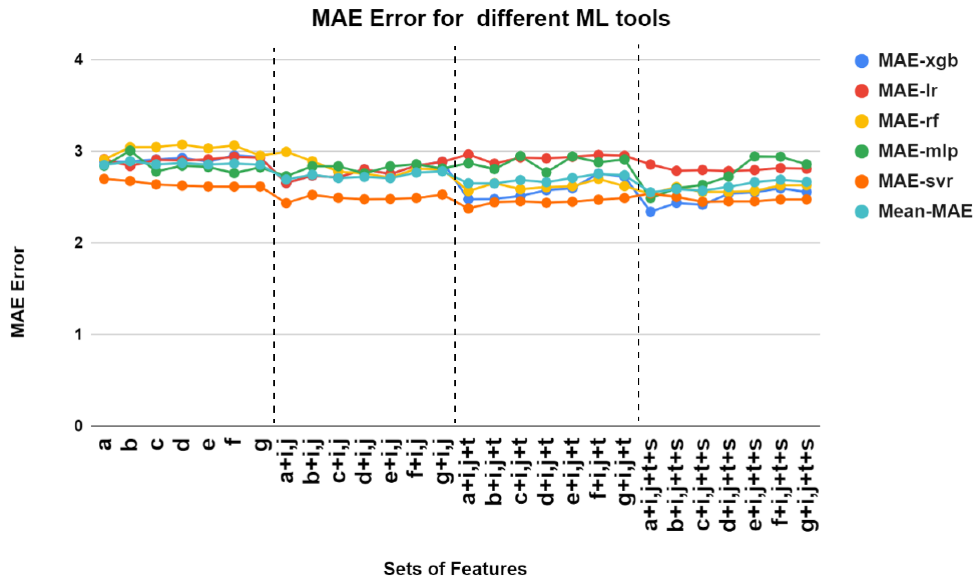
The data in Table 1, Table 2, Table 3 and Table 4 are summarized in Figure 6 and Figure 7. For MAE, XGB with all features (including same-pixel, spatial-temporal, and square root rescaling) gives the overall best performance. However, SVR is clearly the best performer for most feature sets. SVR tends to work best with fewest same-pixel features (i.e., configuration a, which is the previous month + 12 months prior). SVR with configuration a + (i, j) reduces the MAE by about 7% over the best result without spatial features. Adding time stamp and square root rescaling gives little additional improvement. In general, SVR gave MAE values that were between 7 and 20 % better than the worst-performing algorithms, which were random forest (for same-pixel and same-pixel + spatial location feature sets) or linear regression (for other feature sets). It is noteworthy that adding a time stamp brought large error reductions to random forest and XGB, while having little effect on linear regression, MLP, and SVR.
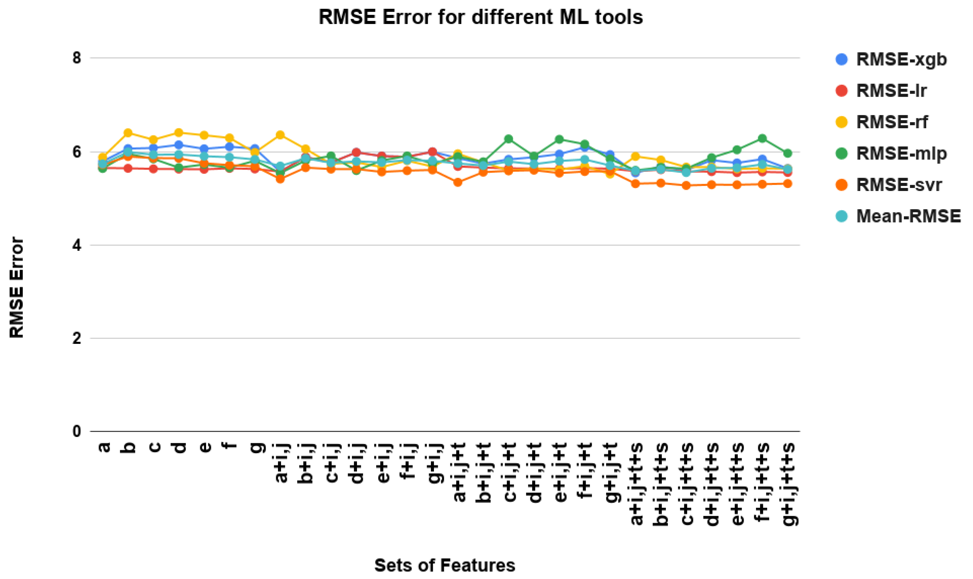
The RMSE results resemble the MAE results in that SVR consistently gives the lowest error. This time however, XGB with a + i, j + t + s does not outperform the SVR results. Once again, same-pixel configuration a tends to give the best results for SVR, and a + i, j has about 4% lower error than a only. In general, SVR gave MAE values that were 2.5–15.5% better than the worst-performing algorithms.
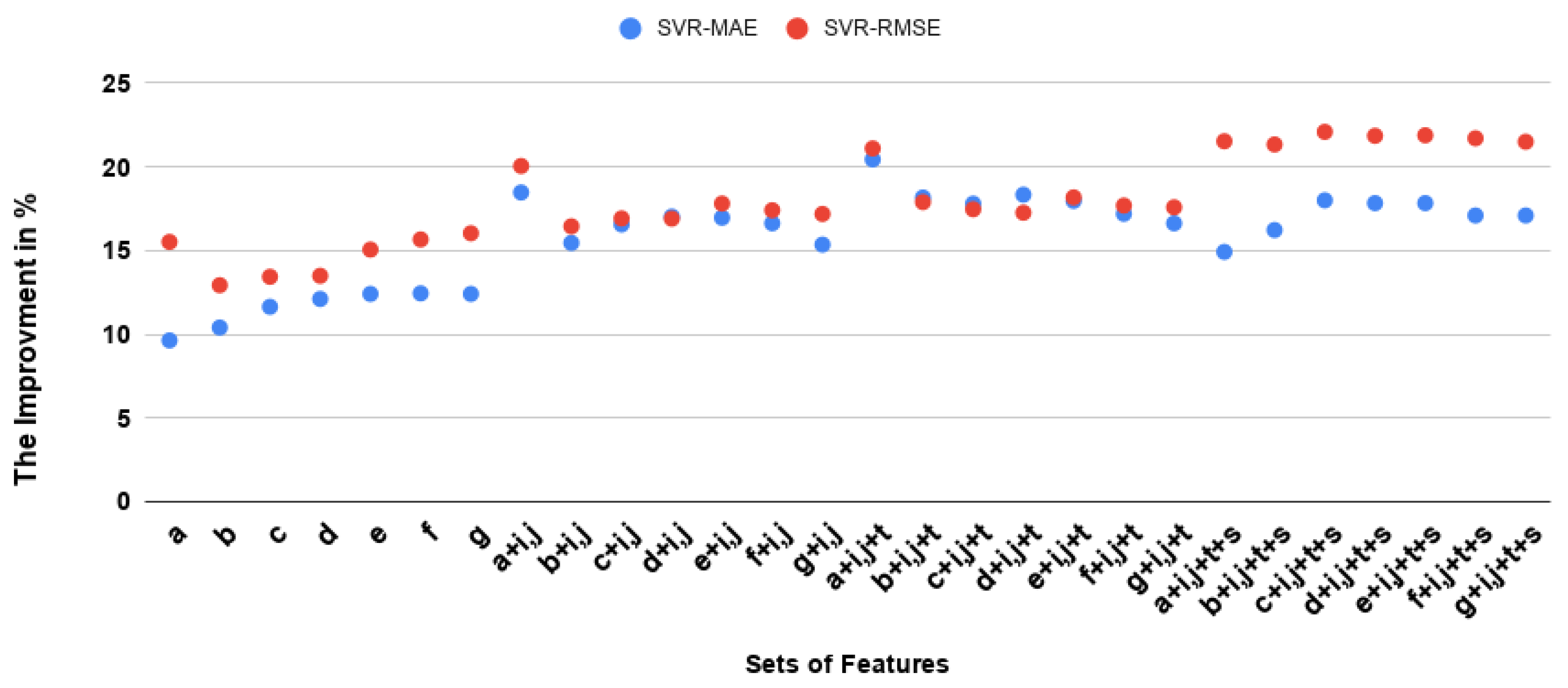
Figure 8, shows the percentage performance improvement (i.e., percentage error reduction) of the overall best-performing model from Table 1, Table 2, Table 3 and Table 4 (SVR) compared to the untrained model based on the previous month. The MAE and RMSE values for the untrained model were 2.988 and 6.771, respectively. When square root rescaling is used, all predictions reduced MAE and RMSE by over 15% and 20%, respectively. The overall best predictor (a + i + j + t) reduced both MAE and RMSE by more than 20%. This result is consistent with [39], which found that SVM outperformed RF when predicting rainfall images up to 3 h ahead on a per-pixel basis.
When GMM was added to XGB with a + i, j + t + s, the values of MAE and RMSE obtained were 2.258 and 4.838, respectively. These values were better than the corresponding best results without GMM by 3.6% and 9.4% respectively. Compared to the untrained predictor, this XGB+GMM model gave 25% improvement in MAE and 29% improvement in RMSE. Figure 9, shows an example of an actual image and its prediction using XGB+GMM.
All of the above results were obtained using the default parameters in sklearn for their respective methods. Parameters were not optimized because of the large number of different methods involved. In particular, optimizing GMM is very expensive since it used 100 trained models which would all have to be optimized separately. We did conduct a preliminary investigation into parameter optimization by tuning parameters used in RF and XGB for the models in Table 1, Table 2 and Table 3. For this purpose, the scikit-optimize package was used, which employs Bayesian optimization. Improvements in MAE and RMSE were less than 6.5%, and still fell short of the performance obtained with GMMs without parameter optimization.
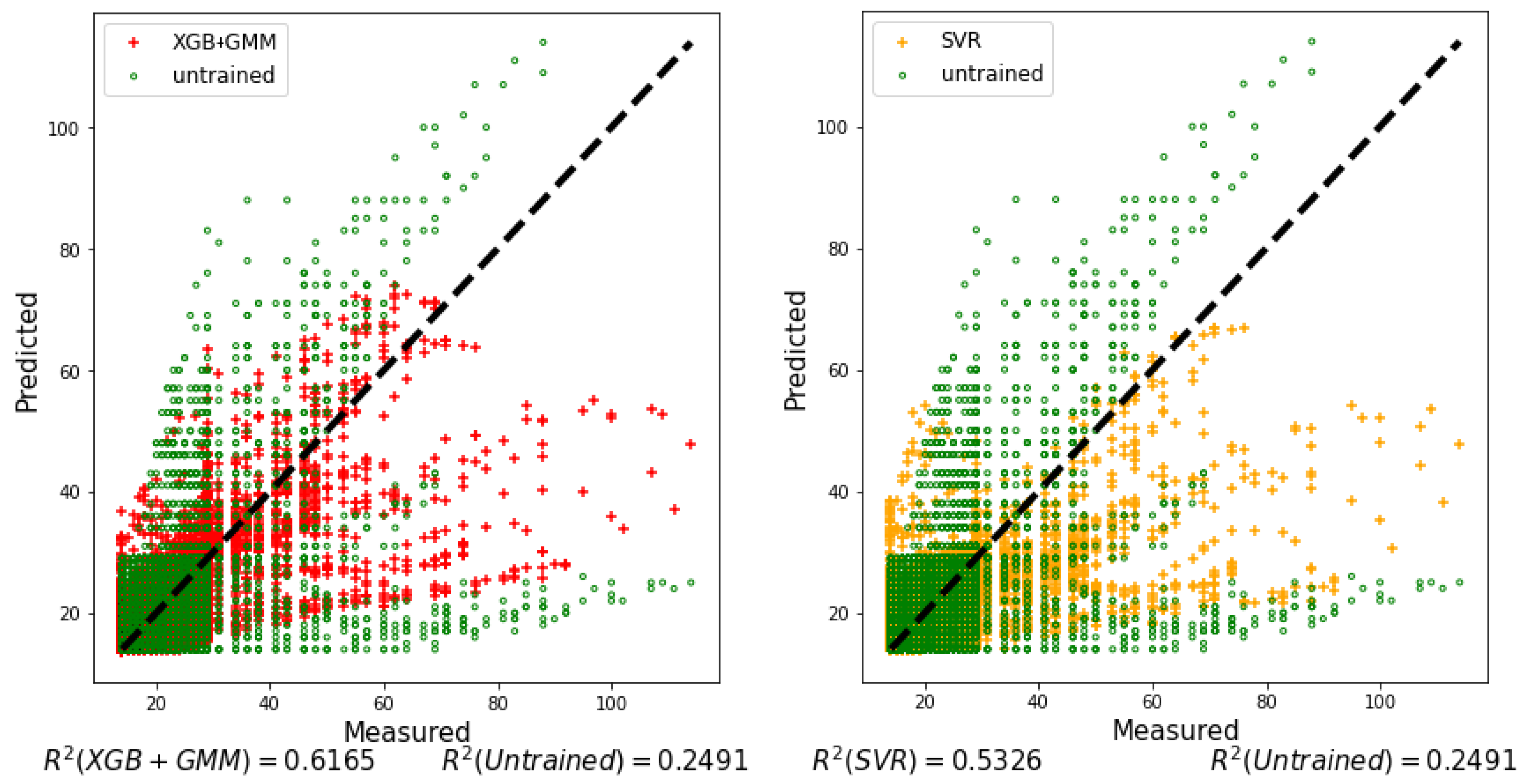
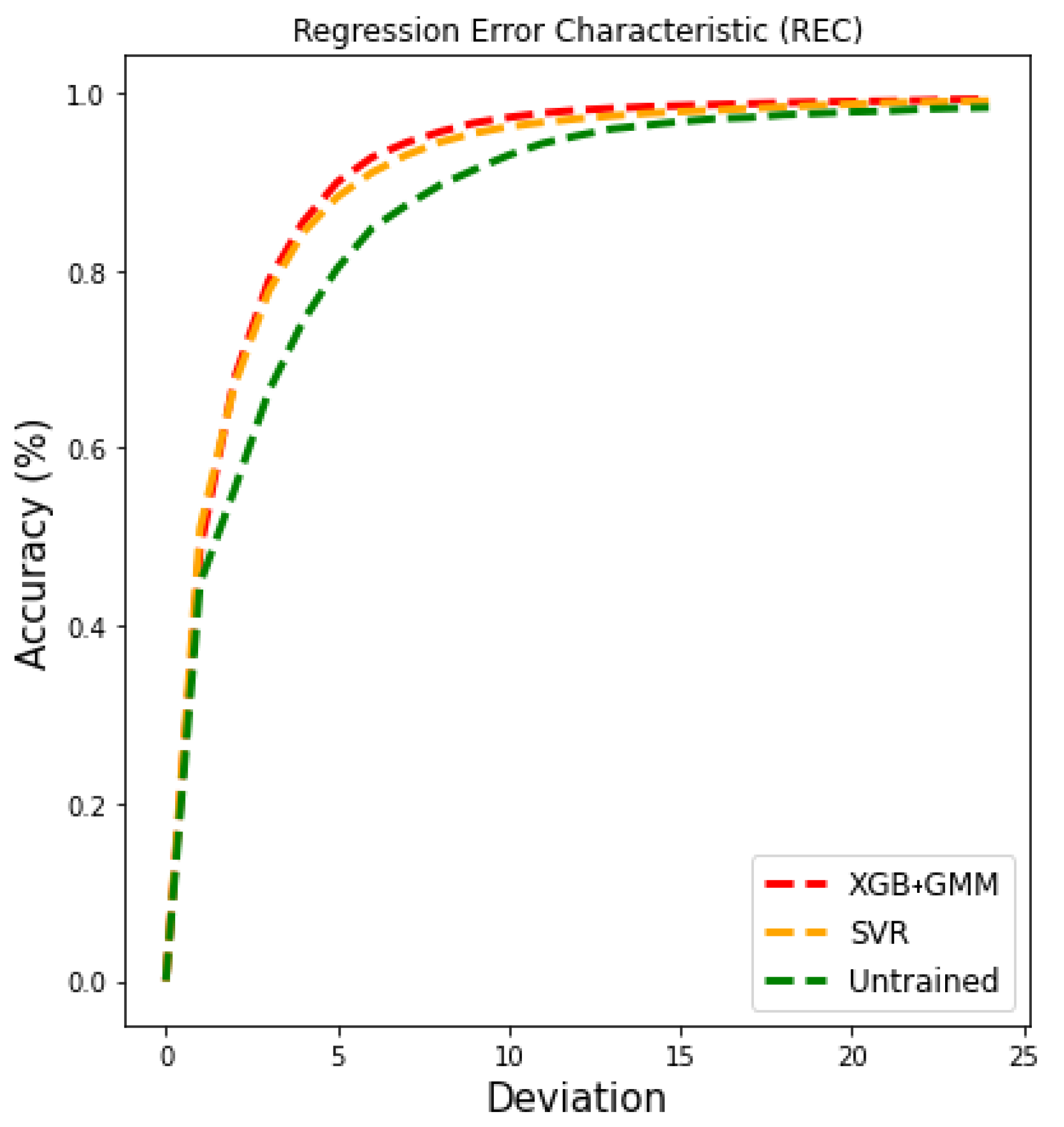
Figure 10 gives residual plots and R 2 values for the best XGB+GMM (a + i, j + t + s) model and the best SVR model (a + i, j + t), superimposed on the untrained model residuals. Visually, XGB+GMM and SVR are giving predictions closer to the 45° line than the untrained regressor, while the R 2 values are more than doubled. Figure 11 presents Regression Error Characteristics (REC) curves for the same three models. For XGB+GMM, 85% of pixel predictions have a deviation of 5 or less.

6. Conclusions

This paper investigated the automatic prediction of groundwater Δ TWS in the GRACE dataset. The proposed approach uses a regression-based approach to predict full groundwater images based on sequences of monthly groundwater maps.
Our results show that the application of appropriate machine-learning techniques can yield significantly more accurate predictions. In particular, it was shown that using SVR as a predictor, automatically selected previous same-pixel values and time stamp as features, and square root rescaling all contributed to better overall prediction outcomes. Global features constructed from GMMs fitted to the pixel intensity distribution brought further improvements.
In future work we will apply these methods to other regions and meteorological parameters such as rainfall, temperature, air pressure, humidity etc. We shall also explore possible improvements to the method such as better imputation of missing values and the investigation of other global features. Additionally, we shall extend these methods to the joint prediction of multiple parameters.

Author Contributions

Conceptualization, M.G., A.B. and E.A.H.; methodology, M.G. and E.A.H.; software, E.A.H.; validation, M.G. and C.T.; formal analysis, C.T.; computing resources, M.G., M.V. and A.B.; writing—original draft preparation, E.A.H.; writing—review and editing, M.G., M.V., C.T. and A.B.; visualization, M.G., C.T. and E.A.H.; supervision, M.G., C.T. and A.B.; funding acquisition, M.G. and M.V. All authors have read and agreed to the published version of the manuscript.

Funding

E.A.H. acknowledges financial support from the South African National Research Foundation, and the Telkom-Openserve-Aria Technologies center of Excellence at Computer Science at UWC.

Acknowledgments

Meerkat Cluster was made use of during this study, (http://docs.meerkat.uwc.ac.za/) provided by the University of the Western Cape’s eRe-search Office (https://eresearch.uwc.ac.za/).

Conflicts of Interest

The authors declare no conflict of interest.

References

  1. Levy, J.; Xu, Y. Groundwater management and groundwater/surface-water interaction in the context of South African water policy. Hydrogeol. J. 2012, 20, 205–226. [Google Scholar] [CrossRef]
  2. Braune, E.; Xu, Y. Groundwater management issues in Southern Africa—An IWRM perspective. Water SA 2008, 34, 699–706. [Google Scholar] [CrossRef] [Green Version]
  3. Ghasemian, D. Groundwater Management Using Remotely Sensed Data in High Plains Aquifer. Ph.D. Thesis, The University of Arizona, Tucson, AZ, USA, 2016. [Google Scholar]
  4. Cao, G.; Zheng, C.; Scanlon, B.R.; Liu, J.; Li, W. Use of flow modeling to assess sustainability of groundwater resources in the North China Plain. Water Resour. Res. 2013, 49, 159–175. [Google Scholar] [CrossRef]
  5. Assembly, U.N.G. Transforming Our World: The 2030 Agenda for Sustainable Development. 2015. Available online: http://www.naturalcapital.vn/wp-content/uploads/2017/02/UNDP-Viet-Nam.pdf (accessed on 15 July 2020).
  6. Felix Landerer. JPL TELLUS GRACE Level-3 Monthly Land Water-Equivalent-Thickness Surface Mass Anomaly Release 6.0 Version 03 in netCDF/ASCII/GeoTIFF Formats; Ver. RL06 v03; PO.DAAC: Pasadena, CA, USA, 2020. [Google Scholar] [CrossRef]
  7. Natkhin, M.; Steidl, J.; Dietrich, O.; Dannowski, R.; Lischeid, G. Differentiating between climate effects and forest growth dynamics effects on decreasing groundwater recharge in a lowland region in Northeast Germany. J. Hydrol. 2012, 448, 245–254. [Google Scholar] [CrossRef]
  8. Goderniaux, P.; Brouyère, S.; Wildemeersch, S.; Therrien, R.; Dassargues, A. Uncertainty of climate change impact on groundwater reserves—Application to a chalk aquifer. J. Hydrol. 2015, 528, 108–121. [Google Scholar] [CrossRef] [Green Version]
  9. Yadav, B.; Ch, S.; Mathur, S.; Adamowski, J. Assessing the suitability of extreme learning machines (ELM) for groundwater level prediction. J. Water Land Dev. 2017, 32, 103–112. [Google Scholar] [CrossRef]
  10. Lo, M.H.; Famiglietti, J.S.; Yeh, P.F.; Syed, T. Improving parameter estimation and water table depth simulation in a land surface model using GRACE water storage and estimated base flow data. Water Resour. Res. 2010, 46. [Google Scholar] [CrossRef]
  11. Zhou, T.; Wang, F.; Yang, Z. Comparative analysis of ANN and SVM models combined with wavelet preprocess for groundwater depth prediction. Water 2017, 9, 781. [Google Scholar] [CrossRef] [Green Version]
  12. Adamowski, J.; Fung Chan, H.; Prasher, S.O.; Ozga-Zielinski, B.; Sliusarieva, A. Comparison of multiple linear and nonlinear regression, autoregressive integrated moving average, artificial neural network, and wavelet artificial neural network methods for urban water demand forecasting in Montreal, Canada. Water Resour. Res. 2012, 48. [Google Scholar] [CrossRef]
  13. Sahoo, S.; Jha, M.K. Groundwater-level prediction using multiple linear regression and artificial neural network techniques: A comparative assessment. Hydrogeol. J. 2013, 21, 1865–1887. [Google Scholar] [CrossRef]
  14. Bourennane, H.; King, D.; Couturier, A. Comparison of kriging with external drift and simple linear regression for predicting soil horizon thickness with different sample densities. Geoderma 2000, 97, 255–271. [Google Scholar] [CrossRef]
  15. Tiwari, M.K.; Adamowski, J. Urban water demand forecasting and uncertainty assessment using ensemble wavelet-bootstrap-neural network models. Water Resour. Res. 2013, 49, 6486–6507. [Google Scholar] [CrossRef]
  16. Arandia, E.; Ba, A.; Eck, B.; McKenna, S. Tailoring seasonal time series models to forecast short-term water demand. J. Water Resour. Plan. Manag. 2016, 142, 04015067. [Google Scholar] [CrossRef] [Green Version]
  17. Mirzavand, M.; Ghazavi, R. A stochastic modelling technique for groundwater level forecasting in an arid environment using time series methods. Water Resour. Manag. 2015, 29, 1315–1328. [Google Scholar] [CrossRef]
  18. Nielsen, A. Practical Time Series Analysis: Prediction with Statistics and Machine Learning; O’Reilly: Sebastopol, CA, USA, 2020. [Google Scholar]
  19. Yoon, H.; Jun, S.C.; Hyun, Y.; Bae, G.O.; Lee, K.K. A comparative study of artificial neural networks and support vector machines for predicting groundwater levels in a coastal aquifer. J. Hydrol. 2011, 396, 128–138. [Google Scholar] [CrossRef]
  20. Sun, A.Y. Predicting groundwater level changes using GRACE data. Water Resour. Res. 2013, 49, 5900–5912. [Google Scholar] [CrossRef]
  21. Emamgholizadeh, S.; Moslemi, K.; Karami, G. Prediction the groundwater level of bastam plain (Iran) by artificial neural network (ANN) and adaptive neuro-fuzzy inference system (ANFIS). Water Resour. Manag. 2014, 28, 5433–5446. [Google Scholar] [CrossRef]
  22. Moosavi, V.; Vafakhah, M.; Shirmohammadi, B.; Behnia, N. A wavelet-ANFIS hybrid model for groundwater level forecasting for different prediction periods. Water Resour. Manag. 2013, 27, 1301–1321. [Google Scholar] [CrossRef]
  23. Dos Santos, C.C.; Pereira Filho, A.J. Water demand forecasting model for the metropolitan area of São Paulo, Brazil. Water Resour. Manag. 2014, 28, 4401–4414. [Google Scholar] [CrossRef]
  24. Huang, F.; Huang, J.; Jiang, S.H.; Zhou, C. Prediction of groundwater levels using evidence of chaos and support vector machine. J. Hydroinform. 2017, 19, 586–606. [Google Scholar] [CrossRef] [Green Version]
  25. Rahaman, M.M.; Thakur, B.; Kalra, A.; Li, R.; Maheshwari, P. Estimating High-Resolution Groundwater Storage from GRACE: A Random Forest Approach. Environments 2019, 6, 63. [Google Scholar] [CrossRef] [Green Version]
  26. Jing, W.; Yao, L.; Zhao, X.; Zhang, P.; Liu, Y.; Xia, X.; Song, J.; Yang, J.; Li, Y.; Zhou, C. Understanding terrestrial water storage declining trends in the Yellow River Basin. J. Geophys. Res. Atmos. 2019, 124, 12963–12984. [Google Scholar] [CrossRef]
  27. Jing, W.; Zhao, X.; Yao, L.; Di, L.; Yang, J.; Li, Y.; Guo, L.; Zhou, C. Can terrestrial water storage dynamics be estimated from climate anomalies? Earth Space Sci. 2020, 7, e2019EA000959. [Google Scholar] [CrossRef] [Green Version]
  28. Sahour, H.; Sultan, M.; Vazifedan, M.; Abdelmohsen, K.; Karki, S.; Yellich, J.A.; Gebremichael, E.; Alshehri, F.; Elbayoumi, T.M. Statistical applications to downscale GRACE-derived terrestrial water storage data and to fill temporal gaps. Remote Sens. 2020, 12, 533. [Google Scholar] [CrossRef] [Green Version]
  29. Mukherjee, A.; Ramachandran, P. Prediction of GWL with the help of GRACE TWS for unevenly spaced time series data in India: Analysis of comparative performances of SVR, ANN and LRM. J. Hydrol. 2018, 558, 647–658. [Google Scholar] [CrossRef]
  30. Seyoum, W.M.; Kwon, D.; Milewski, A.M. Downscaling GRACE TWSA data into high-resolution groundwater level anomaly using machine learning-based models in a glacial aquifer system. Remote Sens. 2019, 11, 824. [Google Scholar] [CrossRef] [Green Version]
  31. Shi, X.; Chen, Z.; Wang, H.; Yeung, D.Y.; Wong, W.K.; Woo, W.C. Convolutional LSTM network: A machine learning approach for precipitation nowcasting. In Proceedings of the Advances in Neural Information Processing Systems, Montreal, Canada, 7–12 December 2015; pp. 802–810. [Google Scholar]
  32. Shi, E.; Li, Q.; Gu, D.; Zhao, Z. A Method of Weather Radar Echo Extrapolation Based on Convolutional Neural Networks. In MultiMedia Modeling (MMM 2018); Schoeffmann, K., Ed.; Springer: Cham, Switzerland, 2018; Volume 10704, pp. 16–28. [Google Scholar]
  33. Shi, X.; Gao, Z.; Lausen, L.; Wang, H.; Yeung, D.Y.; Wong, W.k.; Woo, W.C. Deep learning for precipitation nowcasting: A benchmark and a new model. In Proceedings of the Advances in Neural Information Processing Systems, Long Beach, CA, USA, 4–9 December 2017; pp. 5617–5627. [Google Scholar]
  34. Tran, Q.K.; Song, S.k. Multi-Channel Weather Radar Echo Extrapolation with Convolutional Recurrent Neural Networks. Remote Sens. 2019, 11, 2303. [Google Scholar] [CrossRef] [Green Version]
  35. Wang, Y.; Long, M.; Wang, J.; Gao, Z.; Philip, S.Y. Predrnn: Recurrent neural networks for predictive learning using spatiotemporal lstms. In Proceedings of the Advances in Neural Information Processing Systems, Long Beach, CA, USA, 4–9 December 2017; pp. 879–888. [Google Scholar]
  36. Singh, S.; Sarkar, S.; Mitra, P. A deep learning based approach with adversarial regularization for Doppler weather radar ECHO prediction. In Proceedings of the 2017 IEEE International Geoscience and Remote Sensing Symposium (IGARSS), Fort Worth, TX, USA, 23–28 July 2017; pp. 5205–5208. [Google Scholar]
  37. Chen, L.; Cao, Y.; Ma, L.; Zhang, J. A Deep Learning Based Methodology for Precipitation Nowcasting with Radar. Earth Space Sci. 2020, 7, e2019EA000812. [Google Scholar] [CrossRef] [Green Version]
  38. D’Isanto, A.; Cavuoti, S.; Gieseke, F.; Polsterer, K.L. Return of the features-Efficient feature selection and interpretation for photometric redshifts. Astron. Astrophys. 2018, 616, A97. [Google Scholar] [CrossRef] [Green Version]
  39. Yu, P.S.; Yang, T.C.; Chen, S.Y.; Kuo, C.M.; Tseng, H.W. Comparison of random forests and support vector machine for real-time radar-derived rainfall forecasting. J. Hydrol. 2017, 552, 92–104. [Google Scholar] [CrossRef]
  40. Mukhopadhyay, A.; Shukla, B.P.; Mukherjee, D.; Chanda, B. A novel neural network based meteorological image prediction from a given sequence of images. In Proceedings of the 2011 Second International Conference on Emerging Applications of Information Technology, Kolkata, India, 19–20 February 2011; pp. 202–205. [Google Scholar]
  41. Pedregosa, F.; Varoquaux, G.; Gramfort, A.; Michel, V.; Thirion, B.; Grisel, O.; Blondel, M.; Prettenhofer, P.; Weiss, R.; Dubourg, V.; et al. Scikit-learn: Machine Learning in Python. J. Mach. Learn. Res. 2011, 12, 2825–2830. [Google Scholar]
  42. Khademi, F.; Jamal, S.M.; Deshpande, N.; Londhe, S. Predicting strength of recycled aggregate concrete using artificial neural network, adaptive neuro-fuzzy inference system and multiple linear regression. Int. J. Sustain. Built Environ. 2016, 5, 355–369. [Google Scholar] [CrossRef] [Green Version]
  43. Bengio, Y.; Goodfellow, I.; Courville, A. Deep Learning; MIT Press: New York, NY, USA, 2017; Volume 1. [Google Scholar]
  44. Liakos, K.G.; Busato, P.; Moshou, D.; Pearson, S.; Bochtis, D. Machine learning in agriculture: A review. Sensors 2018, 18, 2674. [Google Scholar] [CrossRef] [Green Version]
  45. Ding, S.; Li, H.; Su, C.; Yu, J.; Jin, F. Evolutionary artificial neural networks: A review. Artif. Intell. Rev. 2013, 39, 251–260. [Google Scholar] [CrossRef]
  46. Kolluru, V.; Ussenaiah, M. A survey on classification techniques used for rainfall forecasting. Int. J. Adv. Res. Comput. Sci. 2017, 8, 226–229. [Google Scholar]
  47. Voyant, C.; Notton, G.; Kalogirou, S.; Nivet, M.L.; Paoli, C.; Motte, F.; Fouilloy, A. Machine learning methods for solar radiation forecasting: A review. Renew. Energy 2017, 105, 569–582. [Google Scholar] [CrossRef]
  48. Liaw, A.; Wiener, M. Classification and regression by randomForest. R News 2002, 2, 18–22. [Google Scholar]
  49. Farnaaz, N.; Jabbar, M. Random forest modeling for network intrusion detection system. Procedia Comput. Sci. 2016, 89, 213–217. [Google Scholar] [CrossRef] [Green Version]
  50. Brownlee, J. XGBoost with Python, 1.10 ed.; Machine Learning Mastery; Machine Learning Mastery Pty: Victoria, Australia, 2018. [Google Scholar]
  51. Hastie, T.; Tibshirani, R.; Friedman, J. The Elements of Statistical Learning: Data Mining, Inference, and Prediction; Springer Science & Business Media: Berlin, Germany, 2009. [Google Scholar]
  52. Chau, K.; Wu, C. A hybrid model coupled with singular spectrum analysis for daily rainfall prediction. J. Hydroinform. 2010, 12, 458–473. [Google Scholar] [CrossRef] [Green Version]
  53. Oğcu, G.; Demirel, O.F.; Zaim, S. Forecasting electricity consumption with neural networks and support vector regression. Procedia Soc. Behav. Sci. 2012, 58, 1576–1585. [Google Scholar] [CrossRef] [Green Version]
  54. Hsu, C.C.; Wu, C.H.; Chen, S.C.; Peng, K.L. Dynamically optimizing parameters in support vector regression: An application of electricity load forecasting. In Proceedings of the 39th Annual Hawaii International Conference on System Sciences (HICSS’06), Kauia, HI, USA, 4–7 January 2006; Volume 2, p. 30c. [Google Scholar]
  55. Cheng, C.S.; Chen, P.W.; Huang, K.K. Estimating the shift size in the process mean with support vector regression and neural networks. Expert Syst. Appl. 2011, 38, 10624–10630. [Google Scholar] [CrossRef]
  56. Zeng, J.; Xie, L.; Liu, Z.Q. Type-2 fuzzy Gaussian mixture models. Pattern Recognit. 2008, 41, 3636–3643. [Google Scholar] [CrossRef]
  57. Reynolds, D.A. Gaussian Mixture Models. 2009. Available online: http://leap.ee.iisc.ac.in/sriram/teaching/MLSP_16/refs/GMM_Tutorial_Reynolds.pdf (accessed on 15 July 2020).
  58. Tran, D.; Le, T.V.; Wagner, M. Fuzzy Gaussian mixture models for speaker recognition. In Proceedings of the Fifth International Conference on Spoken Language Processing, Sydney, Australia, 30 November–4 December 1998. [Google Scholar]
  59. Brassington, G. Mean Absolute Error and Root Mean Square Error: Which Is the Better Metric for Assessing Model Performance? 2017. Available online: https://meetingorganizer.copernicus.org/EGU2017/EGU2017-3574.pdf (accessed on 15 July 2020).
  60. Chai, T.; Draxler, R.R. Root mean square error (RMSE) or mean absolute error (MAE)?—Arguments against avoiding RMSE in the literature. Geosci. Model Dev. 2014, 7, 1247–1250. [Google Scholar] [CrossRef] [Green Version]
  61. Mukhopadhyay, A.; Shukla, B.P.; Mukherjee, D.; Chanda, B. Prediction of meteorological images based on relaxation labeling and artificial neural network from a given sequence of images. In Proceedings of the 2012 International Conference on Computer Communication and Informatics, Coimbatore, India, 10–12 January 2012; pp. 1–5. [Google Scholar]
  62. Mehr, A.D.; Nourani, V.; Khosrowshahi, V.K.; Ghorbani, M.A. A hybrid support vector regression—Firefly model for monthly rainfall forecasting. Int. J. Environ. Sci. Technol. 2019, 16, 335–346. [Google Scholar] [CrossRef]
  63. Nourani, V.; Uzelaltinbulat, S.; Sadikoglu, F.; Behfar, N. Artificial intelligence based ensemble modeling for multi-station prediction of precipitation. Atmosphere 2019, 10, 80. [Google Scholar] [CrossRef] [Green Version]
  64. Fienen, M.N.; Nolan, B.T.; Feinstein, D.T. Evaluating the sources of water to wells: Three techniques for metamodeling of a groundwater flow model. Environ. Model. Softw. 2016, 77, 95–107. [Google Scholar] [CrossRef]
  65. Abudu, S.; Cui, C.; King, J.P.; Moreno, J.; Bawazir, A.S. Modeling of daily pan evaporation using partial least squares regression. Sci. China Technol. Sci. 2011, 54, 163–174. [Google Scholar] [CrossRef]
  66. Pinheiro, A.; Vidakovic, B. Estimating the square root of a density via compactly supported wavelets. Comput. Stat. Data Anal. 1997, 25, 399–415. [Google Scholar] [CrossRef]
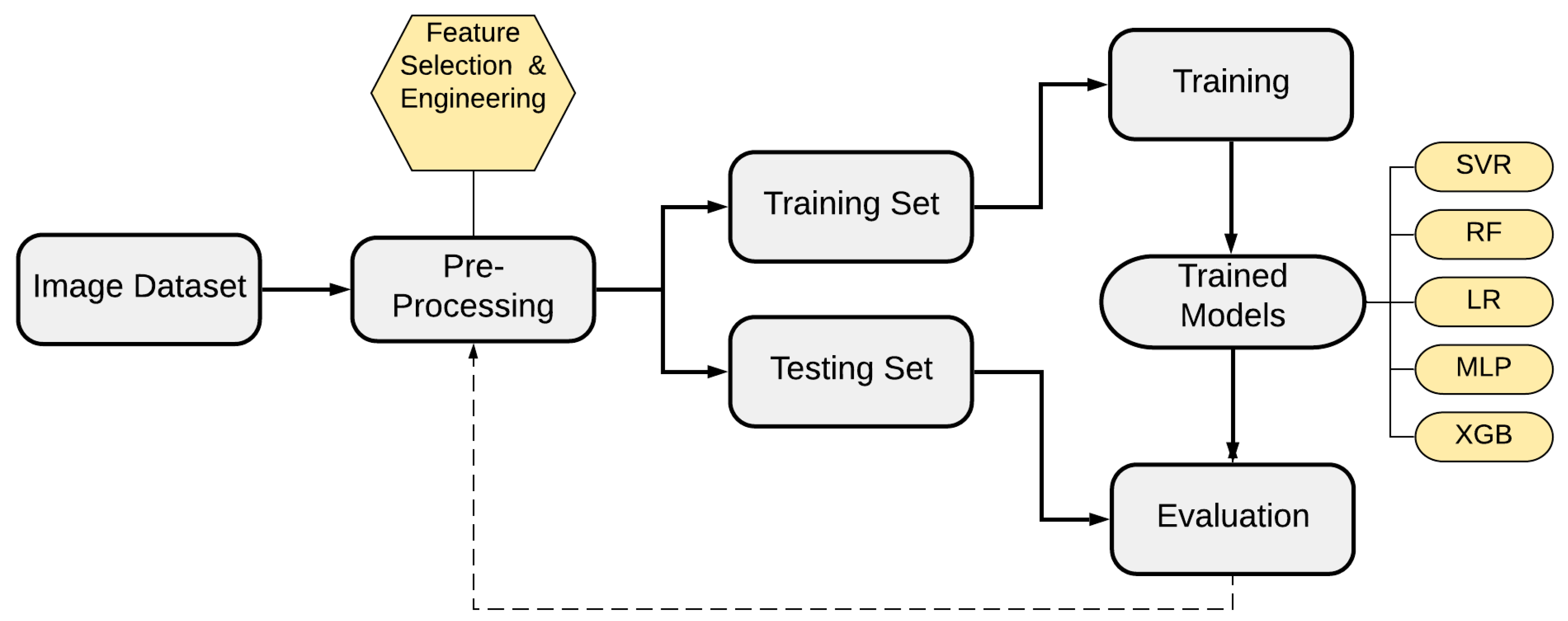
Figure 1. Flowchart showing the implementation process.
Algorithms 13 00300 g001
Figure 2. A sample full image of the GRACE groundwater dataset used in this research [6].
Algorithms 13 00300 g002
Figure 3. Overview of dataset preparation for feature selection: (left) Example of groundwater image of southern Africa before pre-processing (note image is inverted vertically); (right) Notation for same-pixel features used in image prediction.
Algorithms 13 00300 g003
Figure 4. Feature importance of same pixel of previous months, where f(0) stands for same month previous year, and f(11) stands for previous month.
Algorithms 13 00300 g004
Figure 5. Two image representations of groundwater, where (A) represents a normal frame of groundwater; (B) represents the captured high pixels intensity.
Algorithms 13 00300 g005
Figure 6. MAE Graph for the different set configurations.
Algorithms 13 00300 g006
Figure 7. RMSE Graph for the different set configurations.
Algorithms 13 00300 g007
Figure 8. Performance improvement of SVR versus the untrained previous month regressor.
Algorithms 13 00300 g008
Figure 9. Example of an image prediction made with the model (XGB+GMM).
Algorithms 13 00300 g009
Figure 10. Residual plots and R 2 values for XGB+GMM versus untrained predictor (left), and best SVR model versus the untrained (right).
Algorithms 13 00300 g010
Figure 11. Regression error characteristic (REC) curves for the best XGB+GMM, and SVR models, together with the untrained regressor.
Algorithms 13 00300 g011
Table 1. RMSE and MAE for the same-pixel features from previous months, using seven different configurations and five different machine-learning techniques.
FeaturesMAE
XGB
RMSE
XGB
MAE
LR
RMSE
LR
MAE
RF
RMSE
RF
MAE
MLP
RMSE
MLP
MAE
SVR
RMSE
SVR
MAE
Mean
RMSE
Mean
a2.8875.7902.9155.6492.9115.8782.8435.6392.7005.7202.8515.735
b2.8906.0642.8405.6423.0476.4023.0085.9522.6775.8952.8925.991
c2.9126.0782.9095.6303.0486.2552.7825.8442.6405.8612.8585.933
d2.9286.1452.9005.6253.0746.4072.8445.6572.6265.8572.8745.938
e2.8906.0602.9135.6213.0346.3512.8295.7232.6175.7512.8565.901
f2.9576.1042.9425.6413.0656.2932.7635.6552.6165.7102.8685.880
g2.9366.0652.9335.6282.9545.9812.8265.8032.6175.6852.8535.832
Table 2. RMSE and MAE using the same-pixel features from Table 1, plus an additional pixel location feature, using five different machine-learning techniques.
FeaturesMAE
XGB
RMSE
XGB
MAE
LR
RMSE
LR
MAE
RF
RMSE
RF
MAE
MLP
RMSE
MLP
MAE
SVR
RMSE
SVR
MAE
Mean
RMSE
Mean
a + i, j2.6555.5712.6555.5712.9966.3582.735.5402.4365.4132.6945.690
b + i, j2.7365.8842.7365.8842.8936.0572.8385.8092.5265.6572.7455.858
c + i, j2.7165.7632.7165.7632.7815.7362.8385.9082.4935.6252.7085.750
d + i, j2.8055.9832.8055.9832.7595.7702.7605.5942.4795.6262.7215.791
e + i, j2.7535.9042.7535.9042.7145.6682.8385.8092.4815.5652.7075.770
f + i, j2.8445.8902.8445.8902.8115.8062.8605.9072.4915.5922.7705.817
g + i, j2.8875.9962.8875.9962.8045.6792.8135.7422.5295.6072.7845.804
Table 3. RMSE and MAE using the same feature sets as Table 2 plus time stamp, using five different machine-learning techniques.
FeaturesMAE
XGB
RMSE
XGB
MAE
LR
RMSE
LR
MAE
RF
RMSE
RF
MAE
MLP
RMSE
MLP
MAE
SVR
RMSE
SVR
MAE
Mean
RMSE
Mean
a + i, j + t2.4785.8592.9675.6822.5675.9542.8725.8932.3775.3422.6525.746
b + i, j + t2.4815.7422.8675.6582.6535.7692.8075.7812.4455.5592.6505.701
c + i, j + t2.5145.8342.9335.6412.5875.5952.956.2722.4565.5882.6805.786
d + i, j + t2.5765.8792.9245.6372.6095.6342.7715.9032.4405.6022.6605.731
e + i, j + t2.5985.9462.945.6332.6205.6132.9456.2632.4515.5402.7105.799
f + i, j + t2.7586.0922.9625.6452.7005.6892.8826.1592.4745.5732.7555.831
g + i, j + t2.7245.9362.9545.6342.6215.5192.9125.8432.4915.5802.7405.702
Table 4. RMSE and MAE using the same feature sets as Table 3 and square root rescaling, using five different machine-learning techniques.
FeaturesMAE
XGB
RMSE
XGB
MAE
LR
RMSE
LR
MAE
RF
RMSE
RF
MAE
MLP
RMSE
MLP
MAE
SVR
RMSE
SVR
MAE
Mean
RMSE
Mean
a + i, j + t + s2.3425.5442.8575.5822.5365.8972.4905.5982.5425.3132.5535.586
b + i, j + t + s2.4385.6822.7885.6122.6125.8212.5985.6612.5035.3262.5875.620
c + i, j + t + s2.4175.6022.7975.5752.5585.6682.6335.6342.4505.2752.5715.550
d + i, j + t + s2.5395.8162.7855.5712.5575.6702.7265.8702.4555.2912.6125.643
e + i, j + t + s2.5545.7572.7965.5502.5695.6292.9456.0392.4555.2892.6635.652
f + i, j + t + s2.5965.8392.8185.5652.6285.6422.9426.2832.4775.3012.6925.726
g + i, j + t + s2.5575.6392.8115.5532.6315.6322.8595.9642.4775.3152.6675.620
Publisher’s Note: MDPI stays neutral with regard to jurisdictional claims in published maps and institutional affiliations.