Abstract
There are two reasons to have an efficient algorithm for identifying all right-maximal Lyndon substrings of a string: firstly, Bannai et al. introduced in 2015 a linear algorithm to compute all runs of a string that relies on knowing all right-maximal Lyndon substrings of the input string, and secondly, Franek et al. showed in 2017 a linear equivalence of sorting suffixes and sorting right-maximal Lyndon substrings of a string, inspired by a novel suffix sorting algorithm of Baier. In 2016, Franek et al. presented a brief overview of algorithms for computing the Lyndon array that encodes the knowledge of right-maximal Lyndon substrings of the input string. Among those presented were two well-known algorithms for computing the Lyndon array: a quadratic in-place algorithm based on the iterated Duval algorithm for Lyndon factorization and a linear algorithmic scheme based on linear suffix sorting, computing the inverse suffix array, and applying to it the next smaller value algorithm. Duval’s algorithm works for strings over any ordered alphabet, while for linear suffix sorting, a constant or an integer alphabet is required. The authors at that time were not aware of Baier’s algorithm. In 2017, our research group proposed a novel algorithm for the Lyndon array. Though the proposed algorithm is linear in the average case and has worst-case complexity, it is interesting as it emulates the fast Fourier algorithm’s recursive approach and introduces -reduction, which might be of independent interest. In 2018, we presented a linear algorithm to compute the Lyndon array of a string inspired by Phase I of Baier’s algorithm for suffix sorting. This paper presents the theoretical analysis of these two algorithms and provides empirical comparisons of both of their C++ implementations with respect to the iterated Duval algorithm.
1. Introduction
In combinatorics on words, Lyndon words play a very important role. Lyndon words, a special case of Hall words, were named after Roger Lyndon, who was looking for a suitable description of the generators of free Lie algebras [1]. Despite their humble beginnings, to date, Lyndon words have facilitated many applications in mathematics and computer science, some of which are: constructing de Bruijin sequences, constructing bases in free Lie algebras, finding the lexicographically smallest or largest substring in a string, and succinct prefix matching of highly periodic strings; see Marcus et al. [2], and the informative paper by Berstel and Perrin [3] and the references therein.
The pioneering work on Lyndon decomposition was already introduced by Chen, Fox, and Lyndon in [4]. The Lyndon decomposition theorem is not explicitly stated there; nevertheless, it follows from the work presented there.
Theorem 1
(Lyndon decomposition theorem, Chen+Fox+Lyndon, 1958). For any word , there are unique Lyndon words so that for any , and , where ≺ denotes the lexicographic ordering.
As there exists a bijection between Lyndon words over an alphabet of cardinality k and irreducible polynomials over [5], many results are known about this factorization: the average number of factors, the average length of the longest factor [6] and of the shortest [7]. Several algorithms deal with Lyndon factorization. Duval gave in [8] an elegant algorithm that computes, in linear time and in-place, the factorization of a word into Lyndon words. More about its implementation can be found in [9]. In [10], Fredricksen and Maiorana presented an algorithm generating all Lyndon words up to a given length in lexicographical order. This algorithm runs in a constant average time.
Two of the latest applications of Lyndon words are due to Bannai et al. In [11], they employed Lyndon roots of runs to prove the runs conjecture that the number of runs in a string is bounded by the length of the string. In the same paper, they presented an algorithm to compute all the runs in a string in linear time that requires the knowledge of all right-maximal Lyndon substrings of the input string with respect to an order of the alphabet and its inverse. The latter result was the major reason for our interest in computing the right-maximal Lyndon substrings of a given string. Though the terms word and string are interchangeable, and so are the terms subword and substring, in the following, we prefer to use exclusively the terms string and substring to avoid confusing the reader.
There are at least two reasons for having an efficient algorithm for identifying all right-maximal Lyndon substrings of a string: firstly, Bannai et al. published in 2017 [11] a linear algorithm to compute all runs in a string that depends on knowing all right-maximal Lyndon substrings of the input string, and secondly, in 2017, Franek et al. in [12] showed a linear equivalence of sorting suffixes and sorting right-maximal Lyndon substrings, inspired by Phase II of a suffix sorting algorithm introduced by Baier in 2015 (Master’s thesis [13]) and published in 2016 [14].
The most significant feature of the runs algorithm presented in [11] is that it relies on knowing the right-maximal Lyndon substrings of the input string for some order of the alphabet and for the inverse of that order, while all other linear algorithms for runs rely on Lempel–Ziv factorization of the input string. It also raised the issue about which approach may be more efficient: to compute the Lempel–Ziv factorization or to compute all right-maximal Lyndon substrings. There are several efficient linear algorithms for Lempel–Ziv factorization (e.g., see [15,16] and the references therein).
Interestingly, Kosolobov [17] showed that for a general alphabet, in the decision tree model, the runs problem is easier than the Lempel–Ziv decomposition. His result supports the conjecture that there must be a linear random access memory model algorithm finding all runs.
Baier introduced in [13], and published in [14], a new algorithm for suffix sorting. Though Lyndon strings were never mentioned in [13,14], it was noticed by Cristoph Diegelmann in a personal communication [18] that Phase I of Baier’s suffix sort identifies and sorts all right-maximal Lyndon substrings.
The right-maximal Lyndon substrings of a string can be best encoded in the so-called Lyndon array, introduced in [19] and closely related to the Lyndon tree of [20]: an integer array so that for any , the length of the right-maximal Lyndon substring starting at the position i.
In an overview [19], Franek et al. discussed an algorithm based on an iterative application of Duval’s Lyndon factorization algorithm [8], which we refer to here as IDLA, and an algorithmic scheme based on Hohlweg and Reutenauer’s work [20], which we refer to as SSLA. The authors were not aware of Baier’s algorithm at that time. Two additional algorithms were presented there, a quadratic recursive application of Duval’s algorithm and an algorithm NSV* with possibly worst-case complexity based on ranges that can be compared in constant time for constant alphabets. The correctness of NSV* and its complexity were discussed there just informally.
The algorithm IDLA (see Figure 1) is simple and in-place, so no additional space is required except for the storage for the string and the Lyndon array. It is completely independent of the alphabet of the string and does not require the alphabet to be sorted; all it requires is that the alphabet be ordered, i.e., only pairwise comparisons of the alphabet symbols are needed. Its weakness is its quadratic worst-case complexity, which becomes a problem for longer strings with long right-maximal Lyndon substrings, as one of our experiments showed (see Figure 11 in Section 7).
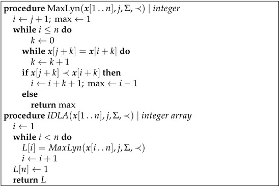
Figure 1.
Algorithm IDLA.
In our empirical work, we used IDLA as a control for comparison and as a verifier of the results. Note that the reason the procedure MaxLyn of Figure 1 really computes the longest Lyndon prefix is not obvious and is based on the properties of periods of prefixes; see [8] or Observation 6 and Lemma 11 in [19].
Lemma 1, below, characterizes right-maximal Lyndon substrings in terms of the relationships of the suffixes and follows from the work of Hohlweg and Reutenauer [20]. Though the definition of the proto-Lyndon substring is formally given in Section 2 below, it suffices to say the it means that it is a prefix of a Lyndon substring of the string. The definition of the lexicographic ordering ≺ is also given Section 2. The proof of this lemma is delayed to the end of Section 2, where all the technical terms needed are defined.
Lemma 1.
Consider a string over an alphabet ordered by ≺.
A substring is proto-Lyndon if and only if:
- (a)
- for any .
A substring is right-maximal Lyndon if and only if:
- (b)
- is proto-Lyndon and
- (c)
- either or .
Thus, the Lyndon array is an NSV (Next Smaller Value) array of the inverse suffix array. Consequently, the Lyndon array can be computed by sorting the suffixes, i.e., computing the suffix array, then computing the inverse suffix array, and then applying NSV to it; see [19]. Computing the inverse suffix array and applying NSV are “naturally” linear, and computing the suffix array can be implemented to be linear; see [19,21] and the references therein. The execution and space characteristics are dominated by those of the first step, i.e., computation of the suffix array. We refer to this scheme as SSLA.
In 2018, a linear algorithm to compute the Lyndon array from a given Burrows–Wheeler transform was presented [22]. Since the Burrows–Wheeler transform is computed in linear time from the suffix array, it is yet another scheme of how to obtain the Lyndon array via suffix sorting: compute the suffix array; from the suffix array, compute the Burrows–Wheeler transform, then compute the Lyndon array during the inversion of the Burrows–Wheeler transform. We refer to this scheme as BWLA.
The introduction of Baier’s suffix sort in 2015 and the consequent realization of the connection to right-maximal Lyndon substrings brought up the realization that there was an elementary (not relying on a pre-processed global data structure such as a suffix array or a Burrows–Wheeler transform) algorithm to compute the Lyndon array, and that, despite its original clumsiness, could be eventually refined to outperform any SSLA or BWLA implementation: any implementation of a suffix sorting-based scheme requires a full suffix sort and then some additional processing, while Baier’s approach is “just” a partial suffix sort; see [23].
In this work, we present two additional algorithms for the Lyndon array not discussed in [19]. The C++ source code of the three implementations IDLA, TRLA, and BSLA is available; see [24]. Note that the procedure IDLA is in the lynarr.hpp file.
The first algorithm presented here is TRLA. TRLA is a -reduction based Lyndon array algorithm that follows Farach’s approach used in his remarkable linear algorithm for suffix tree construction [25] and reproduced very successfully in all linear algorithms for suffix sorting (e.g., see [21,26] and the references therein). Farach’s approach follows the Cooley–Tukey algorithm for the fast Fourier transform relying on recursion to lower the quadratic complexity to complexity; see [27]. TRLA was first introduced by the authors in 2019 (see [28,29]) and presented as a part of Liut’s Ph.D. thesis [30].
The second algorithm, BSLA, is a Baier’s sort-based Lyndon array algorithm. BSLA is based on the idea of Phase I of Baier’s suffix sort, though our implementation necessarily differs from Baier’s. BSLA was first introduced at the Prague Stringology Conference 2018 [23] and also presented as a part of Liut’s Ph.D. thesis [30] in 2019; here, we present a complete and refined theoretical analysis of the algorithm and a more efficient implementation than that initially introduced.
The paper is structured as follows: In Section 2, the basic notions and terminology are presented. In Section 3, the TRLA algorithm is presented and analysed. In Section 4, the BSLA algorithm is presented and analysed. In Section 5, the datasets with random strings of various lengths and over various alphabets and other datasets used in the empirical tests are described. In Section 6, the conclusion of the research and the future work are presented. The results of the empirical measurements of the performance of IDLA, TRLA, and BSLA on those datasets are presented in Section 7 in both tabular and graphical forms.
2. Basic Notation and Terminology
Most of the fundamental notions, definitions, facts, and string algorithms can be found in [31,32,33,34]. For the ease of access, this section includes those that are directly related to the work herein.
The set of integers is denoted by . For two integers , the range. An alphabet is a finite or infinite set of symbols, or equivalently called letters. We always assume that the sentinel symbol $ is not in the alphabet and is always assumed to be lexicographically the smallest. A string over an alphabet is a finite sequence of symbols from . A $-terminated string over is a string over terminated by $. We use the array notation indexing from 1 for strings; thus, indicates a string of length n; the first symbol is the symbol with index 1, i.e., ; the second symbol is the symbol with index 2, i.e., , etc. Thus, . For a $-terminated string of length n, . The alphabet of string , denoted as , is the set of all distinct alphabet symbols occurring in .
We use the term strings over a constant alphabet if the alphabet is a fixed finite alphabet. The integer alphabet is the infinite alphabet . We use the term strings over integer alphabet for the strings over the alphabet with an additional constraint that all letters occurring in the string are all smaller than the length of the string, i.e., in this paper, is a string over the integer alphabet if it is a string over the alphabet . Many authors use a more general definition; for instance, Burkhardt and Kärkkäinen [35] defined it as any set of integers of size ; however, our results can easily be adapted to such more general definitions without changing their essence.
We use a bold font to denote strings; thus, x denotes a string, while x denotes some other mathematical entity such as an integer. The empty string is denoted by and has length zero. The length or size of string is n. The length of a string is denoted by . For two strings and , the concatenation is a string
where
If , then is a prefix, a substring, and a suffix of . If (respectively, , ) is empty, then it is called an empty prefix (respectively, empty substring, empty suffix); if (respectively, , ), then it is called a proper prefix (respectively, proper substring, proper suffix). If , then is called a rotation or a conjugate of ; if either or , then the rotation is called trivial. A non-empty string is primitive if there is no string and no integer so that .
A non-empty string has a non-trivial border if is both a non-empty proper prefix and a non-empty proper suffix of . Thus, both and are trivial borders of . A string without a non-trivial border is call unbordered.
Let ≺ be a total order of an alphabet . The order is extended to all finite strings over the alphabet : for and , if either is a proper prefix of or there is a so that , ..., and . This total order induced by the order of the alphabet is called a lexicographic order of all non-empty strings over . We denote by if either or . A string over is Lyndon for a given order ≺ of if is strictly lexicographically smaller than any non-trivial rotation of . In particular:
x is Lyndon ⇒x is unbordered ⇒ x is primitive
Note that the reverse implications do not hold: is primitive but neither unbordered, nor Lyndon, while is unbordered, but not Lyndon. A substring of , is a right-maximal Lyndon substring of if it is Lyndon and either or for any , is not Lyndon.
A substring of a string is proto-Lyndon if there is a so that is Lyndon. The Lyndon array of a string is an integer array so that where is a maximal integer such that is Lyndon. Alternatively, we can define it as an integer array so that where j is the last position of the right-maximal Lyndon substring starting at the position i. The relationship between those two definitions is straightforward: or .
Proof ofLemma 1.
We first prove the following claim:
Claim. Substring is right-maximal Lyndon if and only if:
- for any and
- either or .
Let be right-maximal Lyndon. We need to show that and hold.
Let . Since it is Lyndon, . Thus, there is so that and and for any and . It follows that , and is satisfied.
If , then holds. Therefore, let us assume that .
- (1)
- If , then ; together with for any , it shows that is Lyndon, contradicting the right-maximality of .
- (2)
- If , then , and holds.
- (3)
- If , then there are a prefix , strings and , and an integer so that , , and . Let us take a maximal such and a maximal such r.
- (3a)
- Let . Then, since is Lyndon, , and so, ; hence, , and holds.
- (3b)
- Let , i.e., and . There is no common prefix of and as it would contradict the maximality of . There are thus two mutually exclusive cases, either or . Let and . If , then , and so, . For any , as is Lyndon, so , giving to be Lyndon, a contradiction with the right-maximality of . Therefore, ; thus, , and holds.
Now, we go in the opposite direction. Assuming and , we need to show that is right-maximal Lyndon.
Consider the right-maximal substring of starting at the position i; it is for some .
- (1)
- If , then by the first part of this proof, , contradicting the assumption as .
- (2)
- If , then , and by the first part of this proof, , contradicting the assumption .
- (3)
- If , then is right-maximal Lyndon.
Now, we can prove . Let be a proto-Lyndon substring of . By definition, it is a prefix of a Lyndon substring of and, hence, a prefix of a right-maximal Lyndon substring of , say for some . It follows from the claim that for any . Since , holds. For the opposite direction, if holds, then there are two possibilities: either there is so that or for any . By the claim, in the former case, is a right-maximal Lyndon substring of , while in the latter case, is a right-maximal Lyndon substring of . Thus, in both cases, is a prefix of a Lyndon substring of .
With proven, we can now replace in the claim with , completing the proof. □
3. -Reduction Algorithm (TRLA)
The purpose of this section is to introduce a recursive algorithm TRLA for computing the Lyndon array of a string. As will be shown below, the most significant aspect is the so-called -reduction of a string and how the Lyndon array of the -reduced string can be expanded to a partially filled Lyndon array for the whole string, as well as how to compute the missing values. This section thus provides the mathematical justification for the algorithm and, in so doing, proves the correctness of the algorithm. The mathematical understanding of the algorithm provides the bases for the bounding of its worst-case complexity by and determining the linearity of the average-case complexity.
The first idea of the algorithm was proposed in Paracha’s 2017 Ph.D. thesis [36]. It follows Farach’s approach [25]:
- (1)
- reduce the input string to ;
- (2)
- by recursion, compute the Lyndon array of ; and
- (3)
- from the Lyndon array of , compute the Lyndon array of .
The input strings for the algorithm are $-terminated strings over an integer alphabet. The reduction computed in (1) is important. All linear algorithms for suffix array computations use the proximity property of suffixes: comparing and can be done by comparing and and, if they are the same, comparing with . For instance, in the first linear algorithm for the suffix array by Kärkkäinen and Sanders [37], obtaining the sorted suffixes for positions and via the recursive call is sufficient to determine the order of suffixes for the positions, then merging both lists together. However, there is no such proximity property for right-maximal Lyndon substrings, so the reduction itself must have a property that helps determine some of the values of the Lyndon array of from the Lyndon array of and computing the rest.
In our algorithm, we use a special reduction, which we call -reduction, defined in Section 3.2, that reduces the original string to at most and at least of its length. The algorithm computes as a -reduction of the input string in Step (1) in linear time. In Step (3), it expands the Lyndon array of the reduced string computed by Step (2) to an incomplete Lyndon array of the original string also in linear time. The incomplete Lyndon array computed in (3) is about to full, and for every position i with an unknown value, the values at positions and are known. In particular, the values at Position 1 and position n are both known. Therefore, much information is provided by the recursive Step (2). For instance, for 00011001, via the recursive call, we would identify the right-maximal Lyndon substrings that are underlined in and would need to compute the missing right-maximal Lyndon substrings that are underlined in .
However, computing the missing values of the incomplete Lyndon array takes at most steps, as we will show, resulting in the overall worst-case complexity of . When the input string is such that the missing values of the incomplete Lyndon array of the input string can be computed in linear time, the overall execution of the algorithm is linear as well, and thus, the average case complexity will be shown to be linear in the length of the input string.
In the following subsections, we describe the -reduction in several steps: first, the -pairing, then choosing the -alphabet, and finally, the computation of the . The -reduction may be of some general interest as it preserves (see Lemma 6) some right-maximal Lyndon substrings of the original string.
3.1. -Pairing
Consider a $-terminated string whose alphabet is ordered by ≺ where and for any . A -pair consists of a pair of adjacent positions from the range . The -pairs are computed by induction:
- the initial -pair is ;
- if is the last -pair computed, then:if thenthe next -pair is set tostopelseif thenstopelseif and thenthe next -pair is set to ; repeat 2.elsethe next -pair is set to ; repeat 2.
Every position of the input string that occurs in some -pair as the first element is labelled black; all others are labelled white. Note that Position 1 is always black, while the last position n can be either black or white; however, the positions and n cannot be simultaneously both black. Note also that most of the -pairs do not overlap; if two -pairs overlap, they overlap in a position i such that and and . The first position and the last position never figure in an overlap of -pairs. Moreover, a -pair can be involved in at most one overlap; for an illustration, see Figure 2; for the formal proof see Lemma 2.
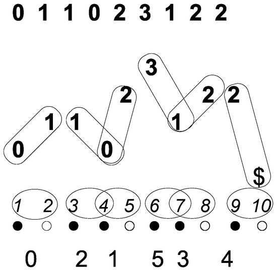
Figure 2.
Illustration of the -reduction of a string 011023122. The rounded rectangles indicate symbol -pairs; the ovals indicate the -pairs. below are the colour labels of the positions; at the bottom is the -reduction.
Lemma 2.
Let be the τpairs of a string . Then, for any :
- (1)
- ,
- (2)
- .
Proof.
This is by induction; trivially true for as is the only -pair. Assume it is true for .
- Case :Then, , and so, are -pairs of ; thus, they satisfy (1) and (2) by the induction hypothesis. However, for , so (1) and (2) hold for .
- Cases and :Therefore, are -pairs of , and thus, they satisfy (1) and (2) by the induction hypothesis. However, for , and ; so, , and so, (1) and (2) hold for .
- Cases and :Then, are -pairs of , so they satisfy (1) and (2) by the induction hypothesis. However, for , so (1) and (2) hold for .
□
3.2. -Reduction
For each -pair , we consider the pair of alphabet symbols . We call them symbol-pairs. They are in a total order ⊲ induced by ≺ : if either , or and . They are sorted using the radix sort with a key of size two and assigned letters from a chosen -alphabet that is a subset of so that the assignment preserves the order. Since the input string is over an integer alphabet, the radix sort is linear.
In the example (Figure 2), the -pairs are , and so, the symbol -pairs are . The sorted symbol -pairs are . Thus, we chose as our -alphabet , and so, the symbol -pairs are assigned these letters: , , , , , and . Note that the assignments respect the order ⊲ of the symbols -pairs and the natural order < of .
The -letters are substituted for the symbol -pairs, and the resulting string is terminated with $. This string is called the -reduction of and denoted , and it is a $-terminated string over an integer alphabet. For our running example from Figure 2, . The next lemma justifies calling the above transformation a reduction.
Lemma 3.
For any string , .
Proof.
There are two extreme cases; the first is when all the -pairs do not overlap at all, then ; and the second is when all the -pairs overlap, then . Any other case must be in between. □
Let denote the set of all black positions of . For any , where j is a black position in of the -pair corresponding to the new symbol in at position i, while assigns each black position of the position in where the corresponding new symbol is, i.e., and . Thus,
In addition, we define p as the mapping of the -pairs to the -alphabet.
In our running example from Figure 2, , , , , , and , while , , , , , and . For the letter mapping, we get , , , , , and .
3.3. Properties Preserved by -Reduction
The most important property of -reduction is a preservation of right-maximal Lyndon substrings of that start at black positions. This means there is a closed formula that gives, for every right-maximal Lyndon substring of , a corresponding right-maximal Lyndon substring of . Moreover, the formula for any black position can be computed in constant time. It is simpler to present the following results using , the alternative form of the Lyndon array, the one where the end positions of right-maximal Lyndon substrings are stored rather than their lengths. More formally:
Theorem 2.
Let ; let be the Lyndon array of ; and let be the Lyndon array of .
Then, for any black , where .
The proof of the theorem requires a series of lemmas that are presented below. First, we show that -reduction preserves the relationships of certain suffixes of .
Lemma 4.
Let , and let . Let and . If i and j are both black positions, then implies .
Proof.
Since i and j are both black positions, both and are defined, and . Let us assume that . The proof is argued in several cases determined by the nature of the relationship .
- (1)
- Case: is a proper prefix of .Then, , and so, . It follows that , and thus, is a border of .
- (1a)
- Case: is black.Since n may be either black or white, we need to discuss two cases.
- (1a)
- Case: n is white.Since n is white, the last -pair of must be . The -pairs of must be the same as the -pairs of ; the last -pair of must be . Since is black by our assumption (1a), the next -pair of must be , as indicated in the following diagram:
 Thus, . Since , we have , and so, is a proper prefix of giving .
 - (1a)
- Case: n is black.Then, the last -pair of must be , and hence, the last -pair of , so the next -pair is ; since cannot be black when n is, the situation is as indicated in the following diagram:
 Thus, . Since and , we have , and so, , giving . Since , we have .
- (1b)
- Case: is white.Then, is black; hence, is black; so, n must also be white, and thus, , as indicated by the following diagram:
 Since , we have , and so, is a proper prefix of , giving .
- (2)
- Case: or ( and ).Then, , and so, , and thus, .
- (3)
- Case: for some , , while .First note that and are either both black, or both are white:
- If is white, then the -pairs of correspond one-to-one to the -pairs of . To determine what follows , we need to know the relationship between the values , , and . Since , , and , the values , , and have the same relationship, and thus, the -pair following will be the “same” as the -pair following . Since is white, the -pair following is , and so, the -pair following is , making white as well.
- If is black, then the -pairs of correspond one-to-one to the -pairs of . It follows that is black as well.
We proceed by discussing these two cases for the colours of and .- (3a)
- Case when and are both white.Therefore, we have the -pairs for that correspond one-to-one to the -pairs for . It follows that . and . Since and, by our assumption (3), , it follows that , giving , and so, . Since and , we have .
- (3b)
- Case when and are both black.Therefore, we have the -pairs for that correspond one-to-one to the -pairs for . It follows that .We need to discuss the four cases based on the colours of and .
- (3b)
- Both and are black.It follows that the next -pair for is , and the next -pair for is . It follows that and . Hence, and . Since and, by Assumption (3), , we have , and so, , giving us . It follows that .
- (3b)
- is white, and is black.It follows that the next -pair for is , and the next -pair for is . It follows that , while . Thus, and . Since is black, we know that . Since and , we have , and so, , as otherwise, would be black. This gives us . Thus, , giving and, ultimately, . The last step is to realize that and , which gives us . It follows that .
- (3b)
- is black, and is white.It follows that the next -pair for is , and the next -pair for is . It follows that , while . Thus, and . Since is black, we know that , where the last inequality is our Assumption (3). Therefore, . Thus, , giving , , and ultimately, . It follows that .
- (3b)
- Both and are white.Then, the next -pair for is , and the next -pair for is . It follows that , while . Thus, and . Since and, by our Assumption (3), , , giving , , and ultimately, . It follows that .
□
Lemma 5 shows that -reduction preserves the proto-Lyndon property of certain proto-Lyndon substrings of .
Lemma 5.
Let , and let . Let . Let be a proto-Lyndon substring of , and let i be a black position.
Then,
Proof.
Let us first assume that j is black.
Since both i and j are black, and are defined. Let , , and consider , so that . Let . Then, and , and so, by Lemma 1 as is proto-Lyndon. It follows that by Lemma 4. Thus, for any , and so, is proto-Lyndon by Lemma 1.
Now, let us assume that j is white.
Then, is black, and is proto-Lyndon, so as in the previous case, is proto-Lyndon. □
Now, we can show that -reduction preserves some right-maximal Lyndon substrings.
Lemma 6.
Let , and let . Let . Let be a right-maximal Lyndon substring, and let i be a black position.
Then,
Proof.
Since is Lyndon and hence proto-Lyndon, by Lemma 5, we know that is proto-Lyndon for j black, while for white j, is proto-Lyndon. Thus, in order to conclude that the respective strings are right-maximal Lyndon substrings, we only need to prove that the property of Lemma 1 holds in both cases.
Since is right-maximal Lyndon, either or by Lemma 1, giving or . Since is Lyndon and hence unbordered, . Thus, either or .
If , then there are two simple cases. If n is white, is black and , so , giving us (c) of Lemma 1 for . On the other hand, if n is black, then , and so, giving us (c) of Lemma 1 for .
Thus, in the following, we can assume that and that . We will proceed by discussing two possible cases, one where j is black and the other where j is white.
- (1)
- Case: j is black.We need to show that either or .If , then , and we are done. Thus, we can assume that . We must show that .
- (1a)
- Case: .Then, and , and so, is black. It follows that . By Lemma 4, because , thus .
- (1b)
- Case: .Then, . It follows that the -pair is followed by a -pair , and thus, . Thus,; hence,. Since , , and , it follows that , and so, .
- (2)
- Case: j is white.We need to prove that . Since j is white, necessarily both and are black and . By Lemma 5, is proto-Lyndon as both i and are black and is proto-Lyndon. Since and both i and are black, by Lemma 4, we get .
□
Now, we are ready to tackle the proof of Theorem 2.
Proof of Theorem 2.
Let where i is black. Then, is defined, and is a right-maximal Lyndon substring of . We proceed by analysis of the two possible cases of the label for the position j. Let (*) denote the condition from the theorem, i.e.,
- (*)
- or
- (1)
- Case: j is black.Then, by Lemma 6, is a right-maximal Lyndon substring of ; hence, . Therefore, . We have to also prove that the condition (*) holds.If , then the condition (*) holds. Therefore, assume that . Since is right-maximal, by Lemma 1, , and so, . Then, .
- (2)
- Case: j is white.Then, is black, and . By Lemma 6, is a right-maximal Lyndon substring of ; hence, , so , giving .We want to show that the condition (*) does not hold.If , then , which is impossible as . Since is Lyndon, , and so, . Thus, Condition (*) does not hold.
□
3.4. Computing from
Theorem 2 indicates how to compute the partial from . The procedure is given in Figure 3.
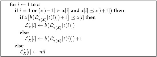
Figure 3.
Computing the partial Lyndon array of the input string.
To compute the missing values, the partial array is processed from right to left. When a missing value at position i is encountered (note that it is recognized by ), the Lyndon array is completely filled, and also, is known. Recall that is the ending position of the right-maximal Lyndon substring starting at the position . In several cases, we can determine the value of in constant time:
- (1)
- if , then .
- (2)
- if , then .
- (3)
- if and and either or , then .
- (4)
- if and and either or , then .
- (5)
- if and and either or , then .
We call such points easy. All others will be referred to as hard. For a hard point i, it means that is followed by at least two consecutive right-maximal Lyndon substrings before reaching either or n, and we might need to traverse them all.
The while loop, seen in Figure 4’s procedure, is the likely cause of the complexity. At first glance, it may seem that the complexity might be ; however, the doubling of the length of the string when a hard point is introduced actually trims it down to an worst-case complexity. See Section 3.5 for more details and Section 7 for the measurements and graphs.
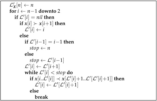
Figure 4.
Computing missing values of the Lyndon array of the input string.
Consider our running example from Figure 2. Since , we have giving . Computing is easy as , and so, . is more complicated and an example of a hard point: we can extend the right-maximal Lyndon substring from to the left to 23, but no more, so . Computing is again easy as , and so, . Thus, .
3.5. The Complexity of TRLA
To determine the complexity of the algorithm, we attach to each position i a counter initialized to zero. Imagine a hard point j indicated by the following diagram:

represents the right-maximal Lyndon substring starting at the position ; represents the right-maximal Lyndon substring following immediately and so forth. To make j a hard point, and . The value of is determined by:
.
To determine the right-maximal Lyndon substring starting at the hard position j, we need first to check if can be left-extended by to make Lyndon; we are using abbreviated notation for the substring where ; in simple words, represents the left-extension of by one position. If is proto-Lyndon, we have to check whether can be left-extended by to a Lyndon substring. If is Lyndon, we must continue until we check whether is Lyndon. If so, we must check whether is Lyndon. We need not go beyond .
How do we check if can left-extend to a Lyndon substring? If , we can stop, and is the right-maximal Lyndon substring starting at position j. If , we need to continue. Since is the last position of the right-maximal Lyndon substring at the position or n, we are assured to stop there. When comparing the substring with , we increment the counter at every position of used in the comparison. When done with the whole array, the value of represents how many times i was used in various comparisons, for any position i.
Consider a position i that was used k times for , i.e., . In the next four diagrams and related text, the upper indices of A and C do not represent powers; they are just indices. The next diagram indicates the configuration when the counter was incremented for the first time in the comparison of and during the computation of the missing value where:
 The next diagram indicates the configuration when the counter was incremented for the second time in the comparison of and during the computation of the missing value where:
 The next diagram indicates the configuration when the counter was incremented for the third time in the comparison of and during the computation of the missing value where:
 The next diagram indicates the configuration when the counter was incremented for the fourth time in the comparison of and during the computation of the missing value where:
 and so forth until the k-th increment of . Thus, if , then as . Thus, , and so, . Thus, either or . Therefore, the overall complexity is .
The next diagram indicates the configuration when the counter was incremented for the second time in the comparison of and during the computation of the missing value where:
The next diagram indicates the configuration when the counter was incremented for the third time in the comparison of and during the computation of the missing value where:
The next diagram indicates the configuration when the counter was incremented for the fourth time in the comparison of and during the computation of the missing value where:
and so forth until the k-th increment of . Thus, if , then as . Thus, , and so, . Thus, either or . Therefore, the overall complexity is .To show that the average case complexity is linear, we first recall that the overall complexity of TRLA is determined by the procedure filling the missing values. We showed above that there are at most missing values (hard positions) that cannot be determined in constant time. We overestimate the number of strings of length n over an alphabet of size , , which will force a non-linear computation, by assuming that every possible subset of indices with any possible letter assignment forces the worst performance. Thus, there are strings that are processed in linear time, say with a constant , and there are strings that are processed in the worst time, with a constant . Let . Then, the average time is bounded by:
for . The last step follows from the fact that for any .
The combinatorics of the processing is too complicated to ascertain whether the worst-case complexity is linear or not. We tried to generate strings that might give the worst performance. We used three different formulas to generate the strings, nesting the white indices that might require non-constant computation: the dataset extreme_trla of binary strings is created using the recursive formula 000, using the first 100 shortest binary Lyndon strings as the start . The moment the size exceeds the required length of the string, the recursion stops, and the string is trimmed to the required length. For the extreme_trla1 dataset, we used the same approach with the formula 00000, and for the extreme_trla2 dataset, we used the formula 000000.
The space complexity of our C++ implementation is bounded by integers. This upper bound is derived from the fact that a Tau object (see Tau.hpp [24]) requires integers of space for a string of length n. Therefore, the first call to TRLA requires , the next recursive call at most , the next recursive call at most , ...; thus, . However, it should be possible to bring it down to integers.
4. The Algorithm BSLA
The purpose of this section is to present a linear algorithm BSLA for computing the Lyndon array of a string over an integer alphabet. The algorithm is based on a series of refinements of a list of groups of indices of the input string. The refinement is driven by a group that is already complete, and the refinement process makes the immediately preceding group also complete. In turn, this newly completed group is used as the driver of the next round of the refinement. In this fashion, the refinement proceeds from right to left until all the groups in the list are complete. The initial list of groups consists of the groups of indices with the same alphabet symbol. The section contains proper definitions of all these terms—group, complete group, and refinement. In the process of refinement, each newly created group is assigned a specific substring of the input string referred to as the context of the group. Throughout the process, the list of the groups is maintained in an increasing lexicographic order by their contexts. Moreover, at every stage, the contexts of all the groups are Lyndon substrings of with an additional property that the contexts of the complete groups are right-maximal Lyndon substrings. Hence, when the refinement is completed, the contexts of all the groups in the list represent all the right-maximal Lyndon substrings of . The mathematics of the process of refinement is necessary in order to ascertain its correctness and completeness and to determine the worst-case complexity of the algorithm.
4.1. Notation and Basic Notions of BSLA
For the sake of simplicity, we fix a string for the whole Section 4.1; all the definitions and the observations apply and refer to this .
A group is a non-empty set of indices of . The group G is assigned a context, i.e., a substring of with the property that for any , . If , then denotes the occurrence of the context of G at the position i, i.e., the substring . We say that a group is smaller than or precedes a group if .
Definition 1.
An ordered list of groups is agroup configurationif:
- ;
- for any ;
- ;
- For any , is a Lyndon substring of .
Note that () and () guarantee that is a disjoint partitioning of . For , denotes the unique group to which i belongs, i.e., if , then . Note that using this notation, .
The mapping is defined by if such j exists, otherwise .
For a group G from a group configuration, we define an equivalence ∼ on G as follows: iff or . The symbol denotes the class of equivalence ∼ that contains i, i.e., . If , then the class is called trivial. An interesting observation states that if G is viewed as an ordered set of indices, then a non-trivial is an interval:
Observation 7.
Let G be a group from a group configuration for . Consider an such that . Let and . Then, .
Proof.
Since is a candidate to be , and , so . □
On each non-trivial class of ∼, we define a relation ≈ as follows: iff ; in simple terms, it means that the occurrence of is immediately followed by the occurrence of . The transitive closure of ≈ is a relation of equivalence, which we also denote by ≈. The symbol denotes the class of equivalence ≈ containing i, i.e., .
For each j from a non-trivial , we define the valence by . In simple terms, is the number of elements from that are . Thus, .
Interestingly, if G is viewed as an ordered set of indices, then is a subinterval of the interval :
Observation 8.
Let G be a group from a group configuration for . Consider an such that . Let and . Then, .
Proof.
We argue by contradiction. Assume that there is an so that and . Take the minimal such j. Consider . Then, , and since, , due to the minimality of j. Therefore, , and so, , a contradiction. □
Definition 2.
A group G iscompleteif for any , the occurrence of is a right-maximal Lyndon substring of .
A group configuration ist-complete, , if
- the groups are complete;
- the mapping isproperon :for any , if and , then there are , , , and so that is a prefix of ;
- the family isproper:if is a proper substring of , i.e., , then ,if is followed immediately by , i.e., when , and , then ;
- the family has theMongeproperty, i.e., if , then or .
The condition is all-important for carrying out the refinement process (see below). The conditions and are necessary for asserting that the condition is preserved during the refinement process.
4.2. The Refinement
For the sake of simplicity, we fix a string for the whole Section 4.2; all the definitions, lemmas, and theorems apply and refer to this .
Lemma 9.
Let and . For , define with context . Then, is a one-complete group configuration.
Proof.
(), (), (), and () are straightforward to verify. To verify (), we need to show that is complete. Any occurrence of in is a right-maximal Lyndon substring, so is complete.
To verify (), consider and for . Consider any r such that . If , then , which contradicts the definition of . Hence, , and so, , while for some . It follows that has as a prefix.
The condition is trivially satisfied as no can have a proper substring. If is immediately followed by and , then , , , and . Then, , so is also satisfied.
To verify (), consider . Then, . □
Let by a t-complete group configuration. The refinement is driven by the group , and it might only partition the groups that precede it, i.e., the groups , while the groups remain unchanged.
- Partition into classes of the equivalence ∼.where may be possibly empty and .
- Partition every class , , into classes of the equivalence ≈.where .
- Therefore, we have a list of classes in this order: , , ... , , , ... , ..., , , ... . This list is processed from left to right. Note that for each , , and .For each , move all elements from the group into a new group H, place H in the list of groups right after the group , and set its context to . (Note, that this “doubling of the contexts” is possible due to . Then, update :
- All values of are correct except possibly the values of for indices from H. It may be the case that for , there is , so that , so must be reset to the maximal such . (Note that before the removal of H from , the index was not eligible to be considered for as i and were both from the same group.)
Theorem 3 shows that having a t-complete group configuration and refining it by , then the resulting system of groups is a -complete group configuration. This allows carrying out the refinement in an iterative fashion.
Theorem 3.
Let be a t-complete group configuration, . After performing the refinement of Conf by group , the resulting system of groups denoted as is a -complete group configuration.
Proof.
We carry the proof in a series of claims. The symbols , , , , and denote the functions for Conf, while , , , , and denote the functions for .
When a group is partitioned, a part of it is moved as the next group in the list, and we call it ; thus, . For details, please see () above.
Claim 1.
is a group configuration, i.e., , , , and for hold.
Proof of Claim 1.
() and () follow from the fact that the process is a refinement, i.e., a group is either preserved as is or is partitioned into two or more groups. The doubling of the contexts in Step guarantees that the increasing order of the contexts is preserved, i.e., () holds. For any so that , is Lyndon, and is also Lyndon, while , so is Lyndon as well; thus, holds.
To illustrate the concatenation: let us call as A and as B, and let , then we know that A is Lyndon and B is Lyndon and ; so, is clearly Lyndon as if A and B were letters. □
This concludes the proof of Claim 1.
Claim 2.
is proper and has the Monge property, i.e., and for hold.
Proof of Claim 2.
Consider for some . There are two possibilities:
- or
- , for some , so that for any , , , and for any and . Note that .
Consider and for some .
- Case and .
- (a)
- Show that holds.If , then , and so, by for Conf, , and thus, . Therefore, for holds.
- (b)
- Show that holds. If , then , so , and so, ; so, for holds.
- Case and ,where , , and .
- (a)
- Show that holds.If , then ; hence, , and so, by for Conf, . By the t-completeness of Conf, is a right-maximal Lyndon substring, a contradiction with being Lyndon. This is an impossible case.
- (b)
- Show that holds.If , then by for Conf. By for Conf, cannot be a suffix of as . Hence, , and so, ; and since cannot be a suffix of as , it follows that , ..., ultimately giving . Therefore, for holds.
- Case and ,where , , and .
- (a)
- Show that holds.If , then either , which implies by for Conf that , giving , or for some . If , then , giving . Therefore for holds.
- (b)
- Show that holds.Let . Consider .Assume that :
- By for Conf, either , and we are done, or . Let be the smallest element of . Since cannot be the prefix of , it means that . Since cannot be a prefix of , it means that , and so, , which contradicts the fact that .
Assume that :- Then, , and so, by for Conf, as .
- Case and ,where , , and and where , , and .
- (a)
- Show that holds.Let . Then, either , and so, , implying that is maximal contradicting being Lyndon. Thus, for some . However, then, , implying that is maximal, again a contradiction. This is an impossible case.
- (b)
- Show that holds.Let . Let us first assume that . Then, . Since cannot be a suffix of , it follows that . Therefore, . Repeating this argument leads to , and we are done.Therefore, assume that . Let be the smallest such that . Such an ℓ must exist. Then, . If , then either is a prefix of or vice versa, both impossibilities; hence, . Repeating the same arguments as for i, we get that , and so, we are done.
It remains to show that for holds.
Consider immediately followed by with .
- Assume that .Then, , , and . If , then , and is immediately followed by , so by for Conf, we have a contradiction. Thus, for and , and is immediately followed by , a contradiction by for Conf.
- Assume that .Then, the group is partitioned when refining by , and so, for . Since is immediately followed by , we have again a contradiction, as it implies that .
□
This concludes the proof of Claim 2.
Claim 3.
The functionis proper on, i.e., for holds.
Proof of Claim 3.
Let and with . Then, , and so, , where . Hence, , , and , and so, . It remains to show that is a prefix of . It suffices to show that is immediately followed by .
If , then by the Monge property , as , and so, by , , a contradiction.
Thus, . Set . It follows that . Assume that . Since and , . Since , . Consider . If , then by , , and so, by , , a contradiction. Thus, . Since immediately follows , by , , a contradiction. Therefore, , and so, is proper on . □
This concludes the proof of Claim 3.
Claim 4.
is a complete group, i.e., for holds.
Proof of Claim 4.
Assume that there is so that is not maximal, i.e., for some , is a right-maximal Lyndon substring of .
Either and so , and so, is a suffix of , or , and then, , since implies that is Lyndon, a contradiction with the right-maximality of . Consider , then , and so, .
Therefore, there is so that , and is a suffix of . Take the smallest such . If , then as is Lyndon. By , , so we have , a contradiction.
Therefore, . Consider . If , is Lyndon, and since , would be a context of , this contradicts the fact was chosen to be the smallest such one. Therefore, , and so, . Thus, there is , , and is a suffix of . Take the smallest such . If , then by , , a contradiction. Hence, . If , then , and so, by , , a contradiction. Hence, .
The same argument done for can now be done for . We end up with and with . If , then we have a contradiction, so . These arguments can be repeated only finitely many times, and we obtain so that , which is a contradiction.
Therefore, our initial assumption that is not maximal always leads to a contradiction. □
This concludes the proof of Claim 4.
The four claims show that all the conditions ... are satisfied for , and that proves Theorem 3.
As the last step, we show that when the process of refinement is completed, all right-maximal Lyndon substrings of are identified and sorted via the contexts of the groups of the final configuration.
Theorem 4.
Let with , , , , and be the initial 1complete group configuration from Lemma 9.
Let with , , , , and be the 2complete group configuration obtained from through the refinement by the group .
Let with , , , , and be the 3complete group configuration obtained from through the refinement by the group .
...
Let with , , , , and be the rcomplete group configuration obtained from through the refinement by the group . Let be the final configuration after the refinement runs out.
Then, is a right-maximal Lyndon substring of iff .
Proof.
That all the groups of are complete follows from Theorem 3, and hence, every is a right-maximal Lyndon string. Let be a right-maximal Lyndon substring of . Consider ; since it is maximal, it must be equal to . □
4.3. Motivation for the Refinement
The process of refinement is in fact a process of the gradual revealing of the Lyndon substrings, which we call the water draining method:
- (a)
- lower the water level by one;
- (b)
- extend the existing Lyndon substrings; the revealed letters are used to extend the existing Lyndon substrings where possible, or became Lyndon substrings of length one otherwise;
- (c)
- consolidate the new Lyndon substrings; processed from the right, if several Lyndon substrings are adjacent and can be joined to a longer Lyndon substring, they are joined.
The diagram in Figure 5 and the description that follows it illustrate the method for a string 011023122. The input string is visualized as a curve, and the height at each point is the value of the letter at that position.
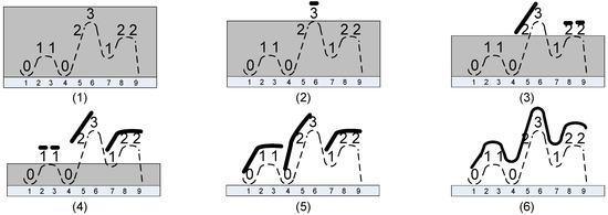
Figure 5.
The water draining method for 011023122. Stages (1)–(6) explained in the text.
In Figure 5, we illustrate the process:
- (1)
- We start with the string 011023122 and a full tank of water.
- (2)
- We drain one level; only 3 is revealed; there is nothing to extend, nothing to consolidate.
- (3)
- We drain one more level, and three 2’s are revealed; the first 2 extends 3 to 23, and the remaining two 2’s form Lyndon substrings 2 of length one; there is nothing to consolidate.
- (4)
- We drain one more level, and three 1’s are revealed; the first two 1’s form Lyndon substrings 1 of length one; the third 1 extends 22 to 122; there is nothing to consolidate.
- (5)
- We drain one more level, and two 0’s are revealed; the first 0 extends 11 to 011; the second 0 extends 23 to 023; in the consolidation phase, 023 is joined with 122 to form a Lyndon substring 023122, and then, 011 is joined with 023122 to form a Lyndon substring 011023122.
Therefore, during the process, the following right-maximal Lyndon substrings were identified: 3 at Position 6, 23 at Position 5, 2 at Positions 8 and 9, 1 at Positions 2 and 3, 122 at Position 7, 023 at Position 4, and finally, 011023122 at Position 1. Note that all positions are accounted for; we really have all right-maximal Lyndon substrings of the string 011023122.
In Figure 6, we present an illustrative example for the string 011023122, where the arrows represent the mapping shown only on the group used for the refinement. The groups used for the refinement are indicated by the bold font.
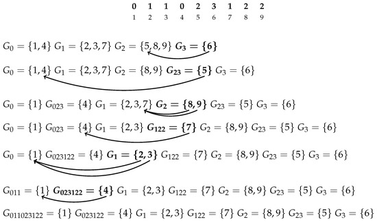
Figure 6.
Group refinement for 011023122.
4.4. The Complexity of BSLA
The computation of the initial configuration can be done in linear time. To compute the initial value of in linear time, a stack-based approach similar to the NSV algorithm is used. Since all groups are non-empty, there can never be more groups than n. Theorem 3 is at the heart of the algorithm. The refinement by the last completed group is linear in the size of the group, including the update of . Therefore, the overall worst-case complexity of BSLA is linear in the length of the input string.
5. Data and Measurements
Initially, computations were performed on the Department of Computing and Software’s moore server; memory: 32 GB (DDR4 @ 2400 MHz), CPU: 8 × Intel Xeon E5-2687W v4 @ 3.00 GHz, OS: Linux Version 2.6.18-419.el5 (gcc Version 4.1.2 and Red Hat Version 4.1.2-55). To verify correctness, new randomized data were produced and computed independently on the University of Toronto Mississauga’s octolab cluster; memory: 8 × 32 GB (DDR4 @ 3200 MHz), CPU: 8 × AMD Ryzen Threadripper 1920X (12-Core) @ 4.00 GHz, OS: Ubuntu 16.04.6 LTS (gcc Version 5.4.0). The results of both were extremely similar, and those reported herein are those generated using the moore server. All the programs were compiled without any additional level of optimization (i.e., neither -O1, nor -O2, nor -O3 flags were specified for the compilation). The CPU time was measured in clock ticks with 1,000,000 clock ticks per second. Since the execution time was negligible for short strings, the processing of the same string was repeated several times (the repeat factor varied from , for strings of length 10, to one, for strings of length ), resulting in a higher precision. Thus, for graphing, the logarithmic scale was used for both, x-axis representing the length of the strings and y-axis representing the time. We used four categories of randomly generated datasets:
- (1)
- binrandom strings over an integer alphabet with exactly two distinct letters (kind of binary strings).
- (2)
- dnarandom strings over an integer alphabet with exactly four distinct letters (kind of random DNA strings).
- (3)
- engrandom strings over an integer alphabet with exactly 26 distinct letters (kind of random English).
- (4)
- intrandom strings over an integer alphabet (i.e., over the alphabet ).
Each dataset contains 100 randomly generated strings of the same length. For each category, there were datasets for length s 10, 50, , , ..., , , , and . The minimum, average, and maximum times for each dataset were computed. Since the variance for each dataset was minimal, the results for minimum times and the results for maximum times completely mimicked the results for the average times, so we only present the averages here.
Tables 1–4 and the graphs in Figures 7–10 from Section 7 clearly indicate that the performance of the three algorithms is linear and virtually indistinguishable. We expected IDLA and TRLA to exhibit linear behaviour on random strings as such strings tend to have many, but short right-maximal Lyndon substrings. However, we did not expect the results to be so close.
Despite the fact that IDLA performed in linear time on the random strings, it is relatively easy to force it into its worst quadratic performance. The dataset extreme_idla contains individual strings of the required lengths. Table 5 and the graph in Figure 11 from Section 7 show this clearly.
In Section 3.5, we describe how the three datasets, extreme_trla, extreme_trla1, and extreme_trla2, are generated and why. The results of experimenting with these datasets do not suggest that the worst-case complexity for TRLA is . Yet again, the performances of the three algorithms are linear and virtually indistinguishable; see Tables 6–8 and the graphs in Figures 12–14 in Section 7.
6. Conclusions and Future Work
We present two novel algorithms for computing right-maximal Lyndon substrings. The first one, TRLA, has a simple implementation with a complicated theory behind it. Its average time complexity is linear in the length of the input string, and its worst-case complexity is no worse than . The -reduction used in the algorithm is an interesting reduction preserving right-maximal Lyndon substrings, a fact used significantly in the design of the algorithm. Interestingly, it seem to slightly outperform BSLA, at least on the datasets used for our experimentations. BSLA, the second algorithm, is linear and elementary in the sense that it does not require a pre-processed global data structure. Being linear and elementary, BSLA is more interesting, and it is possible that its performance could be more streamlined. However, both the theory and implementation of BSLA are rather complex.
On random strings, none of the two algorithms were significantly better than the simple IDLA, whose implementation is just a few lines. However, its quadratic worst-case complexity is an obstacle, as our experiments indicated.
Additional effort needs to go into proving TRLA’s worst-case complexity. The experiments performed did not indicate that it is not linear even in the worst case. Both algorithms need to be compared to some efficient implementation of SSLA and BWLA.
7. Results
This section contains the measurements of the average times for the datasets discussed in the previous section. For better understanding of the data, we present them in Table 1, Table 2, Table 3, Table 4, Table 5, Table 6, Table 7 and Table 8 and Figure 7, Figure 8, Figure 9, Figure 10, Figure 11, Figure 12, Figure 13 and Figure 14. All the graphs include the curve for reference.

Table 1.
Average times for dataset bin ( clock ticks per second).
Table 2.
Average times for dataset dna ( clock ticks per second).
Table 3.
Average times for dataset eng ( clock ticks per second).
Table 4.
Average times for dataset int ( clock ticks per second).
Table 5.
Average times for dataset extreme_idla ( clock ticks per second).
Table 6.
Average times for dataset extreme_trla ( clock ticks per second).
Table 7.
Average times for dataset extreme_trla1 ( clock ticks per second).
Table 8.
Average times for dataset extreme_trla2 ( clock ticks per second).
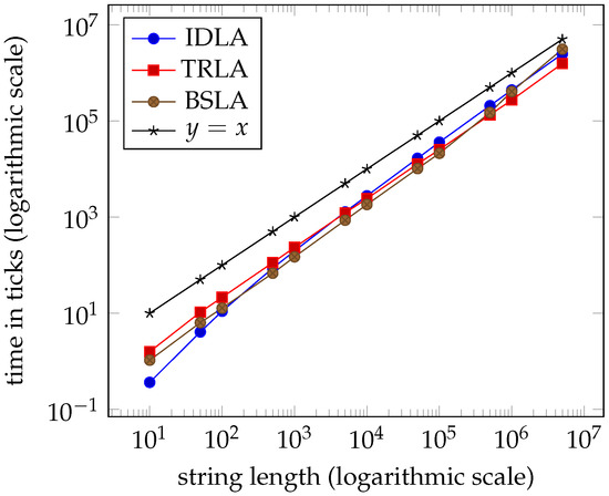
Figure 7.
Average times for dataset bin ( clock ticks per second).
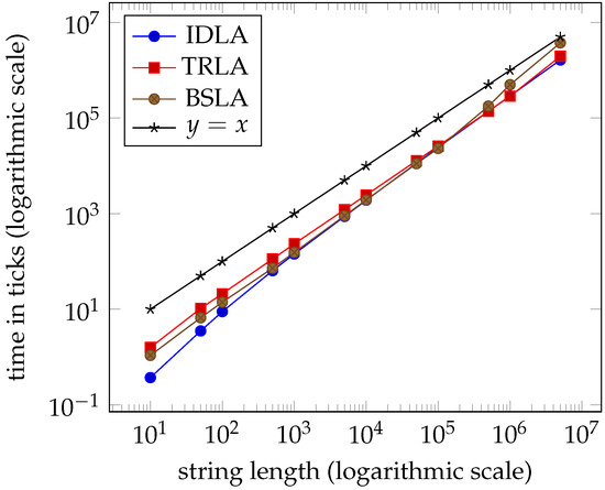
Figure 8.
Average times for dataset dna ( clock ticks per second).
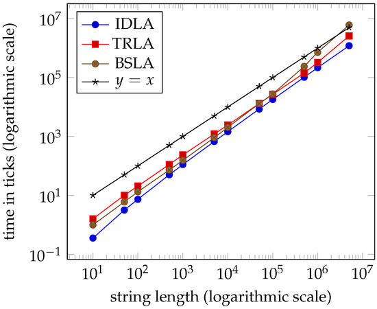
Figure 9.
Average times for dataset eng ( clock ticks per second).
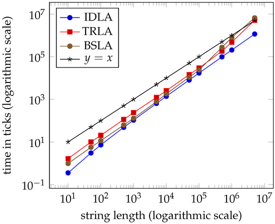
Figure 10.
Average times for dataset int ( clock ticks per second).
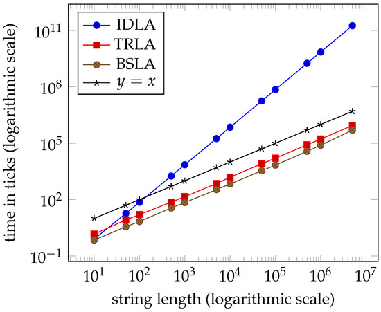
Figure 11.
Average times for dataset extreme_idla ( clock ticks per second).
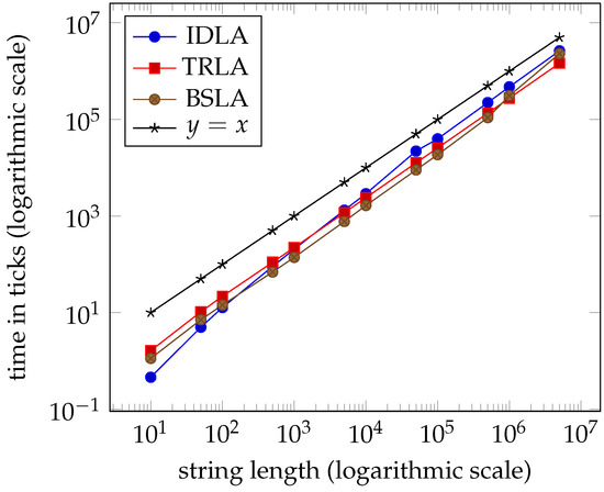
Figure 12.
Average times for dataset extreme_trla ( clock ticks per second).
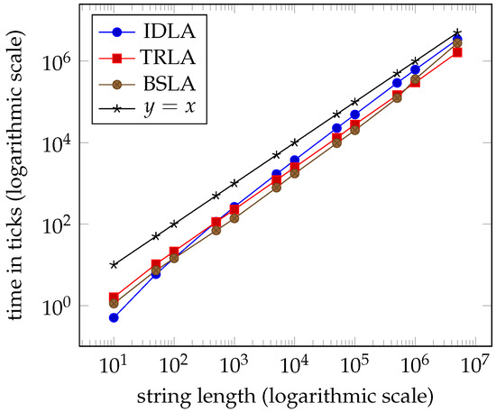
Figure 13.
Average times for dataset extreme_trla1 ( clock ticks per second).
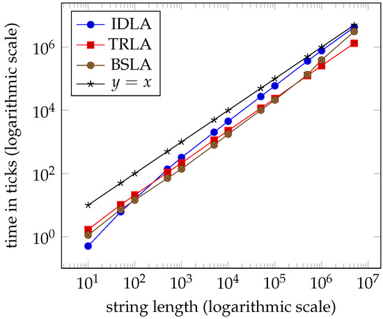
Figure 14.
Average times for dataset extreme_trla2 ( clock ticks per second).
Author Contributions
Conceptualization, F.F. and M.L.; methodology, F.F. and M.L.; software, F.F. and M.L.; validation, F.F. and M.L.; formal analysis, F.F. and M.L.; investigation, F.F. and M.L.; resources, F.F. and M.L.; data curation, F.F. and M.L.; writing, original draft preparation, F.F. and M.L.; writing, review and editing, F.F. and M.L.; visualization, F.F. and M.L.; supervision, F.F. and M.L.; project administration, F.F. and M.L.; funding acquisition, F.F. Both authors read and agreed to the published version of the manuscript.
Funding
This research was funded by the National Sciences and Research Council of Canada (NSERC) Grant RGPIN/5504-2018.
Conflicts of Interest
The authors declare no conflict of interest.
Abbreviations
The following abbreviations are used in this manuscript:
| BSLA | Baier’s Sort Lyndon Array |
| IDLA | Iterative Duval Lyndon Array |
| TRLA | Tau Reduction Lyndon Array |
References
- Lyndon, R.C. On Burnside’s Problem. II. Trans. Am. Math. Soc. 1955, 78, 329–332. [Google Scholar]
- Marcus, S.; Sokol, D. 2D Lyndon words and applications. Algorithmica 2017, 77, 116–133. [Google Scholar] [CrossRef][Green Version]
- Berstel, J.; Perrin, D. The origins of combinatorics on words. Eur. J. Comb. 2007, 28, 996–1022. [Google Scholar] [CrossRef]
- Chen, K.; Fox, R.; Lyndon, R. Free differential calculus IV. The quotient groups of the lower central series. Ann. Math. 2nd Ser. 1958, 68, 81–95. [Google Scholar] [CrossRef]
- Golomb, S. Irreducible polynomials, synchronizing codes, primitive necklaces and cyclotomic algebra. Comb. Math. Appl. 1967, 4, 358–370. [Google Scholar]
- Flajolet, P.; Gourdon, X.; Panario, D. The complete analysis of a polynomial factorization algorithm over finite fields. J. Algorithms 2001, 40, 37–81. [Google Scholar] [CrossRef]
- Panario, D.; Richmond, B. Smallest components in decomposable structures:exp-log class. Algorithmica 2001, 29, 205–226. [Google Scholar] [CrossRef]
- Duval, J.P. Factorizing words over an ordered alphabet. J. Algorithms 1983, 4, 363–381. [Google Scholar] [CrossRef]
- Berstel, J.; Pocchiola, M. Average cost of Duval’s algorithm for generating Lyndon words. Theor. Comput. Sci. 1994, 132, 415–425. [Google Scholar] [CrossRef]
- Fredricksen, H.; Maiorana, J. Necklaces of beads in k colors and k-ary de Bruijn sequences. Discret. Math. 1983, 23, 207–210. [Google Scholar] [CrossRef]
- Bannai, H.; Tomohiro, I.; Inenaga, S.; Nakashima, Y.; Takeda, M.; Tsuruta, K. The “Runs” Theorem. SIAM J. Comput. 2017, 46, 1501–1514. [Google Scholar] [CrossRef]
- Franek, F.; Paracha, A.; Smyth, W. The linear equivalence of the suffix array and the partially sorted Lyndon array. In Proceedings of the Prague Stringology Conference, Prague, Czech Republic, 28–30 August 2017; pp. 77–84. [Google Scholar]
- Baier, U. Linear-Time Suffix Sorting—A New Approach for Suffix Array Construction. Master’s Thesis, University of Ulm, Ulm, Germany, 2015. [Google Scholar]
- Baier, U. Linear-Time Suffix Sorting—A New Approach for Suffix Array Construction. In Proceedings of the 27th Annual Symposium on Combinatorial Pattern Matching (CPM 2016), Tel Aviv, Israel, 27–29 June 2016; Grossi, R., Lewenstein, M., Eds.; Schloss Dagstuhl–Leibniz-Zentrum fuer Informatik: Dagstuhl, Germany, 2016; Volume 54, pp. 1–12. [Google Scholar]
- Chen, G.; Puglisi, S.; Smyth, W. Lempel-Ziv factorization using less time & space. Math. Comput. Sci. 2013, 1, 605–623. [Google Scholar]
- Crochemore, M.; Ilie, L.; Smyth, W. A simple algorithm for computing the Lempel-Ziv factorization. In Proceedings of the 18th Data Compression Conference, Snowbird, UT, USA, 25–27 March 2008; pp. 482–488. [Google Scholar]
- Kosolobov, D. Lempel-Ziv factorization may be harder than computing all runs. In Proceedings of the 32 International Symposium on Theoretical Aspects of Computer Science—STACS 2015, Garching, Germany, 4–7 March 2015; pp. 582–593. [Google Scholar]
- Digelmann, C.; (Frankfurt, Germany). Personal communication, 2016.
- Franek, F.; Sohidull Islam, A.; Sohel Rahman, M.; Smyth, W. Algorithms to compute the Lyndon array. In Proceedings of the Prague Stringology Conference 2016, Prague, Czech Republic, 29–31 August 2016; pp. 172–184. [Google Scholar]
- Hohlweg, C.; Reutenauer, C. Lyndon words, permutations and trees. Theor. Comput. Sci. 2003, 307, 173–178. [Google Scholar] [CrossRef]
- Nong, G.; Zhang, S.; Chan, W.H. Linear suffix array construction by almost pure induced-sorting. In Proceedings of the 2009 Data Compression Conference, Snowbird, UT, USA, 16–18 March 2009; pp. 193–202. [Google Scholar]
- Louza, F.; Smyth, W.; Manzini, G.; Telles, G. Lyndon array construction during Burrows–Wheeler inversion. J. Discret. Algorithms 2018, 50, 2–9. [Google Scholar] [CrossRef]
- Franek, F.; Liut, M.; Smyth, W. On Baier’s sort of maximal Lyndon substrings. In Proceedings of the Prague Stringology Conference 2018, Prague, Czech Republic, 27–28 August 2018; pp. 63–78. [Google Scholar]
- C++ Code for IDLA, TRLA and BSLA Algorithms. Available online: https://github.com/MichaelLiut/Computing-LyndonArray (accessed on 3 November 2020).
- Farach, M. Optimal suffix tree construction with large alphabets. In Proceedings of the 38th IEEE Symp. Foundations of Computer Science, Miami Beach, FL, USA, 20–22 October 1997; pp. 137–143. [Google Scholar]
- Nong, G. Practical linear-time O(1)-workspace suffix sorting for constant alphabets. ACM Trans. Inf. Syst. 2013, 31, 1–15. [Google Scholar] [CrossRef]
- Cooley, J.; Tukey, J. An algorithm for the machine calculation of complex Fourier series. Math. Comput. 1965, 19, 297–301. [Google Scholar] [CrossRef]
- Franek, F.; Liut, M. Computing Maximal Lyndon Substrings of a String, AdvOL Report 2019/2, McMaster University. Available online: http://optlab.mcmaster.ca//component/option,com_docman/task,cat_view/gid,77/Itemid,92 (accessed on 1 March 2019).
- Franek, F.; Liut, M. Algorithms to compute the Lyndon array revisited. In Proceedings of the Prague Stringology Conference 2019, Prague, Czech Republic, 26–28 August 2019; pp. 16–28. [Google Scholar]
- Liut, M. Computing Lyndon Arrays. Ph.D. Thesis, McMaster University, Hamilton, ON, Canada, 2019. [Google Scholar]
- Lothaire, M. Combinatorics on Words; Cambridge University Press: Cambridge, UK, 2003. [Google Scholar]
- Lothaire, M. Applied Combinatorics on Words; Cambridge University Press: Cambridge, UK, 2005. [Google Scholar]
- Smyth, B. Computing Patterns in Strings; Pearson Addison-Wesley: Boston, MA, USA, 2003. [Google Scholar]
- Louza, F.; Gog, S.; Telles, G. Construction of Fundamental Data Structures for Strings; Springer: Cham, Switzerland, 2020. [Google Scholar]
- Burkhardt, S.; Kärkkäinen, J. Fast Lightweight Suffix Array Construction and Checking. In Proceedings of the 14th Annual Conference on Combinatorial Pattern Matching, Michoacan, Mexico, 25–27 June 2003; Springer: Berlin, Heidelberg, 2003; pp. 55–69. [Google Scholar]
- Paracha, A. Lyndon Factors and Periodicities in Strings. Ph.D. Thesis, McMaster University, Hamilton, ON, Canada, 2017. [Google Scholar]
- Kärkkäinen, J.; Sanders, P. Simple linear work suffix array construction. In Proceedings of the 30th International Conference on Automata, Languages and Programming, Eindhoven, The Netherlands, 30 June–4 July 2003; Springer: Berlin/Heidelberg, Germany, 2003; pp. 943–955. [Google Scholar]


Publisher’s Note: MDPI stays neutral with regard to jurisdictional claims in published maps and institutional affiliations. |
© 2020 by the authors. Licensee MDPI, Basel, Switzerland. This article is an open access article distributed under the terms and conditions of the Creative Commons Attribution (CC BY) license (http://creativecommons.org/licenses/by/4.0/).