Markov Chain Monte Carlo Based Energy Use Behaviors Prediction of Office Occupants

Abstract

Prediction of energy use behaviors is a necessary prerequisite for designing personalized and scalable energy efficiency programs. The energy use behaviors of office occupants are different from those of residential occupants and have not yet been studied as intensively as residential occupants. This paper proposes a method based on Markov chain Monte Carlo (MCMC) to predict the energy use behaviors of office occupants. Firstly, an indoor electrical Internet of Things system (IEIoTS) for the office scenario is developed to collect the switching state time series data of selected user electrical equipment (desktop computer, water dispenser, light) and the historical environment parameters. Then, the Metropolis–Hastings (MH) algorithm is used to sample and obtain the optimal solution of the parameters for the office occupants’ behavior function, the model of which includes the energy action model, energy working hours model, and air-conditioner energy use behavior model. Finally, comparative experiments are carried out to evaluate the performance of the proposed method. The experimental results show that while the mean value performs similarly in estimating the energy use model, the proposed method outperforms the Maximum Likelihood Estimation (MLE) method on uncertainty quantification with relatively narrower confidence intervals.

1. Introduction

Building energy consumption has increased dramatically due to population growth, increased demand for building functions, and global climate change in recent decades [1]. The proportion of building energy consumption in China has increased to about 35 percent, in which office building energy consumption occupies an important part [2]. A large number of studies show that building energy consumption is not only affected by meteorological parameters, building shape, envelope structure, window-to-wall ratio, etc., it is also related to the behaviors of occupants [3]. By mining the hidden patterns from office occupants’ equipment usage data and establishing a corresponding personnel energy use behavior model, the most preferred equipment control scheme according to the needs of users can be recommended and configured, and the experience of the office occupants can be improved and accurate demand response strategies for office buildings designed accordingly.

Many scholars have made considerable contributions in the field of personal behavior prediction and have obtained some excellent research results, some of which were reviewed in [4]. The traditional methods of personal behavior prediction mainly include naive Bayes (NB) [5], support vector machine (SVM) [6], k-nearest neighbor (KNN) [7], the hidden Markov model (HMM) [8], and convolutional neural networks (CNN) [9]. Withanage et al. [10] used the depth cuboid similarity feature (DCSF) algorithm to identify and predict the behavior characteristics of the elderly through video capture of personnel behavior information. Although this method has high accuracy, it is easy to invade privacy, and it has low security. Zou et al. [11,12] proposed a personal behavior prediction system based on wearable devices and smart phones. The system can acquire personal information through embedded sensor devices and realize the functions of personal location and behavior prediction. This method improves the prediction accuracy, but the calculation speed is slower due to the increase of the computational complexity of multi-parameter prediction. Kasteren et al. [13,14,15] could predict personal continuous behavior by continuously optimizing the hidden Markov model (HMM), using each sensor activation as a personal action, and simulating the relationship between each action. Chen et al. [16,17,18] used the sequence probability map model to predict single user activity in a wireless sensor network environment, which shortened the identification time and improved the accuracy. Cameras, mobile phones, wearable devices, etc., are all non-intrusive devices, which are prone to cause security problems and fail to meet people’s privacy requirements.

Hitherto, several non-intrusive behavioral prediction methods have been proposed to address some of the above mentioned challenges. Zhou et al. [19] monitored the lighting energy consumption of office buildings in Beijing and Hong Kong for a long time, which was used to study the energy consumption pattern of lighting and simulate lighting behaviors. They found that the fluctuation of daily lighting energy consumption in office buildings is closely related to personal regular routines. Indraganti et al. [20,21] investigated the thermal comfort level of the population and the adaptive behavior of high temperature, in which the polynomial was fitted to the air-conditioning usage rate and outdoor temperature. Wang et al. [22] proposed a basic research framework and quantitative description method for occupant behavior related to building energy. It was based on the segmentation probability function and the conditional triggering form of the personal action model. This method effectively reflected a number of characteristics including the diversity among different individuals, the randomness of behavior, the environmental relevance, and the diversity among different individuals. Kumagai et al. [23] established a quantitative stochastic model based on user actions to predict the air-conditioning usage status. The mathematical descriptions affecting the use of air-conditioning were regarded as a series of conditional probabilities, which had a high accuracy rate. Glicksman et al. [24] proposed a new method for describing personal behavior and built an energy using behavior model and algorithm process based on the “subject and event mechanism”. This model focused on the overall process of people in buildings from mobile behavior to energy use behavior. Influenced by the surrounding physical environment, social environment, and personal subjective factors, such as emotional changes, habit adjustments, etc., the behaviors of office occupants have a large degree of uncertainty. The traditional point prediction models cannot describe them well, while probabilistic models can provide more information about the uncertainty.

This paper proposes an MCMC based method for predicting office occupants’ energy use behavior. The on-off state data of electrical equipment and indoor environmental parameters are collected through the indoor electrical Internet of Things system (IEIoTS). The Metropolis–Hastings MCMC algorithm is used for random sampling of the parameter values of the fitting function, and the sampling theorem is used for judgment, so as to obtain the optimal energy use action model, energy use working hours model, and air-conditioning energy use behavior model of the office occupants. Compared with other prediction approaches, this method can predict the user behavior more quickly, because the accept-reject step in Metropolis–Hastings MCMC algorithms can make the probability distribution model converge more efficiently to the optimal parameters. Understanding users’ energy use behaviors can provide decision-making reference for intelligent control of building equipment. For example, air-conditioners and water dispensers in the office can be turned on automatically during electricity price valley periods and maintained in the specified state in advance before working, which can effectively reduce the electricity bill while providing users with a comfortable working environment.

The rest of the paper is organized as follows: Section 2 introduces the properties of the Markov chain and the principle of the Metropolis–Hastings (MH) MCMC algorithm. Section 3 presents the procedure of the proposed method to predict energy use behaviors of office occupants. The comparative experiments are carried out and the results are discussed in Section 4. Finally, conclusions are drawn in Section 5.

2. Methodology

The Markov chain Monte Carlo (MCMC) method has been widely used in machine learning, deep learning, natural language processing, and others [25]. The MCMC method consists of two MCs. The first MC is Monte Carlo sampling, and the second MC is the Markov chain. It is essentially a method of repeatedly drawing the random values of the assumed parameters according to the current value until it converges to the the real distribution. The samples of each value are randomly sampled, while the selection of values is limited only by the current state and the prior distribution of the assumed parameters [26,27,28,29].

2.1. Markov Chain

In the Markov chain, the probability of state transition from the current state to the next state depends only on its current state, independent of the previous states [30]. Suppose $\cdots ,x_{i-3},x_{i-2},x_{i-1},x_i,\cdots$ are the states in a Markov chain. The transition probability can be described as by:

$$P\left(x_i\right|\cdots ,x_{i-3},x_{i-2},x_{i-1})=P\left(x_i\right|x_{i-1})$$

(1)

where P is the probability of the occurrence of the event; $P\left(x_i\right|x_{i-1})$ is the probability of transitioning to the state $x_i$ under the condition of $x_{i-1}$.

A Markov chain that satisfies the detailed balance condition can converge to a stationary distribution, and it is given by:

$$\pi \left(x^{\left(i\right)}\right)T\left(x^{\left(i-1\right)}\left|x^{\left(i\right)}\right.\right)=\pi \left(x^{\left(i-1\right)}\right)T\left(x^{\left(i\right)}\left|x^{\left(i-1\right)}\right.\right)$$

(2)

where $\pi \left(x\right)$ is the stationary distribution of the system; $\pi \left(x^{\left(i\right)}\right)$ represents the probability value corresponding to the current state; $T\left(x\right)$ is the transfer matrix; $T\left(x^{\left(i\right)}\right|x^{(i-1)})$ is the transition probability from state $i-1$ to i. The existence of this property makes the Markov chain have a recurrence; therefore, the state of the Markov chain can return to any state with a probability greater than zero when the value of the variable iis large enough [31]. A Markov chain that satisfies the detailed balance condition can be converted from the $i-1$ state to i for any two states and without any loss in the conversion. However, under normal circumstances, the two state transitions in the Markov chain are not equal and do not satisfy the detailed balance condition. How to construct the transfer matrix so that the stationary distribution is the target distribution is the key of Markov chain sampling.

2.2. Metropolis–Hastings Algorithm

The Metropolis–Hastings (MH) algorithm is the cornerstone of Markov chain Monte Carlo sampling [32]. In order to make the Markov chain meet the detailed balance condition, the acceptance rate $r(x^{(i-1)},x^{\left(i\right)})$ is introduced to make the original Markov chain jump from state $i-1$ to i, which is received with the probability of $r(x^{(i-1)},x^{\left(i\right)})$[33]. The original Markov chain is random. Assuming there is a stationary distribution of $\pi \left(x\right)$, x is a sample obtained from the Markov chain, and the ratio of $\pi \left(x^{\left(i\right)}\right)$ and $\pi \left(x^{(i-1)}\right)$ can be calculated by Equation (2), while parameters $x^{\left(i\right)}$ and $x^{(i-1)}$ can be selected according to a certain probability. The parameters by multiple iteration sampling should be met $\pi \left(x\right)$ [34,35]. The iterative steps of the MH algorithm are as follows:

• The MH algorithm takes random values in the parameter space as the starting parameter $x^{\left(0\right)}$. The random parameter $x^{\left(1\right)}$ is generated from the distribution function of parameters, and the probability density of the current parameter is calculated.
• First, a random number ${\mu }_t$ is extracted from the uniform distribution of $[0,1]$, and then, we determine whether to keep the current parameter according to whether the probability density ratio between the current parameter $x^{\left(i\right)}$ and the starting parameter $x^{(i-1)}$ is greater than ${\mu }_t$. If the reception probability of the current parameter is greater than ${\mu }_t$, ${\mu }_t\le r(x^{(i-1)},x^{\left(i\right)})$, the state is accepted, and it needs to be updated $x^{\left(i\right)}=x^{\left(i\right)}$, otherwise $x^{\left(i\right)}=x^{(i-1)}$[36]. The acceptance probability $r(x^{(i-1)},x^{\left(i\right)})$ of MH can be described as:

  $$r\left(x^{\left(i-1\right)},x^{\left(i\right)}\right)=min\left\{1,\frac{{\pi }^{\left(x^{\left(i-1\right)}\right)}T\left(x^{\left(i\right)}\left|x^{\left(i-1\right)}\right.\right)}{{\pi }^{\left(x^{\left(i\right)}\right)}T\left(x^{\left(i-1\right)}\left|x^{\left(i\right)}\right.\right)}\right\}$$

  (3)

It is obvious that the acceptance probability $r(x^{(i-1)},x^{\left(i\right)})$ value is between $[0,1]$, and its purpose is accelerating the convergence of the Markov chain to the detailed balance condition.

3. Proposed Method

The energy use behavior of the office occupant has a certain regularity, which is related to the working time and thermal comfort of users. The daily on and off states and working hours of electrical equipment are related to personal energy use behavior habits, and the energy use behavior of air-conditioner is related to users’ thermal comfort. The purpose of this paper is to predict the office occupant energy use behavior by mining the user’s equipment usage data. This method regards the energy use behavior model as a time or temperature function and uses the MCMC method to fit the posterior probability distribution of the energy use action model, energy use working hours model, and air conditioning energy use behavior model. The prediction process of personnel energy use behavior can be roughly divided into three sections: data acquisition, data preprocessing, and model training.

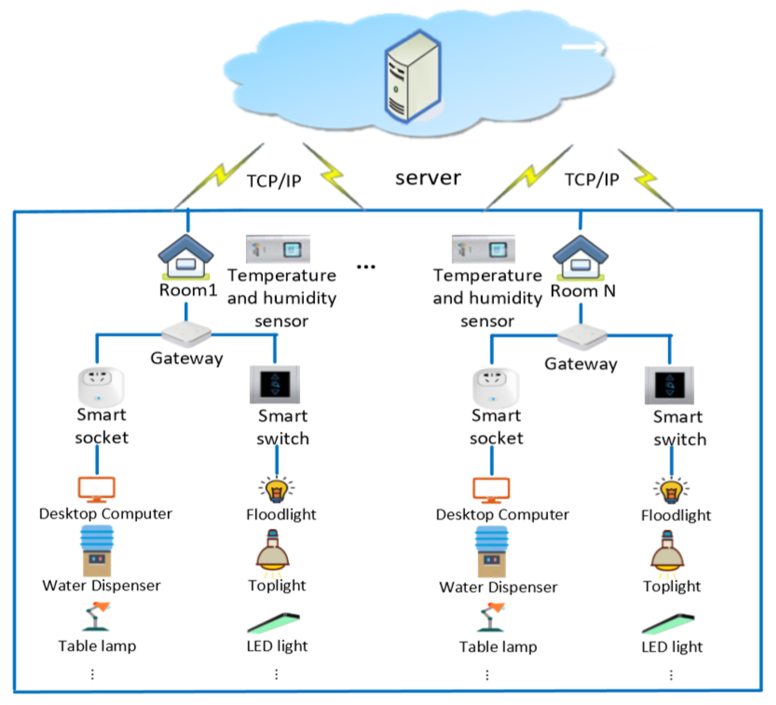
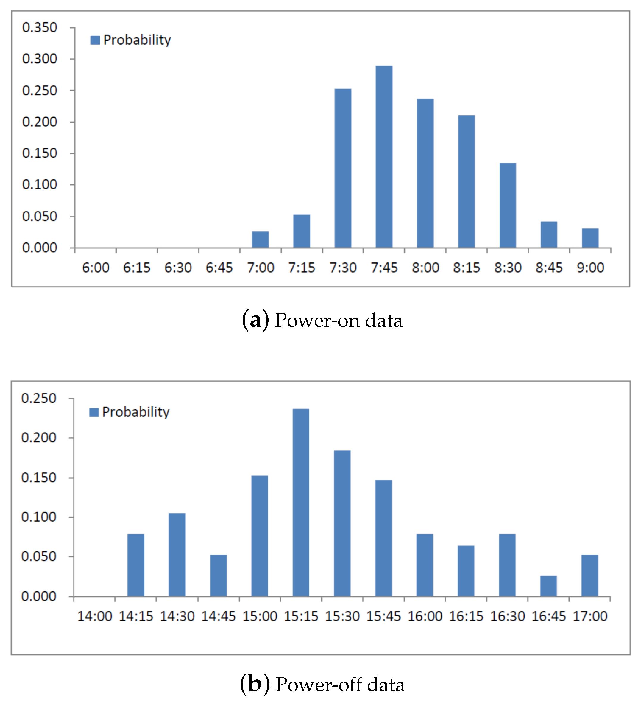
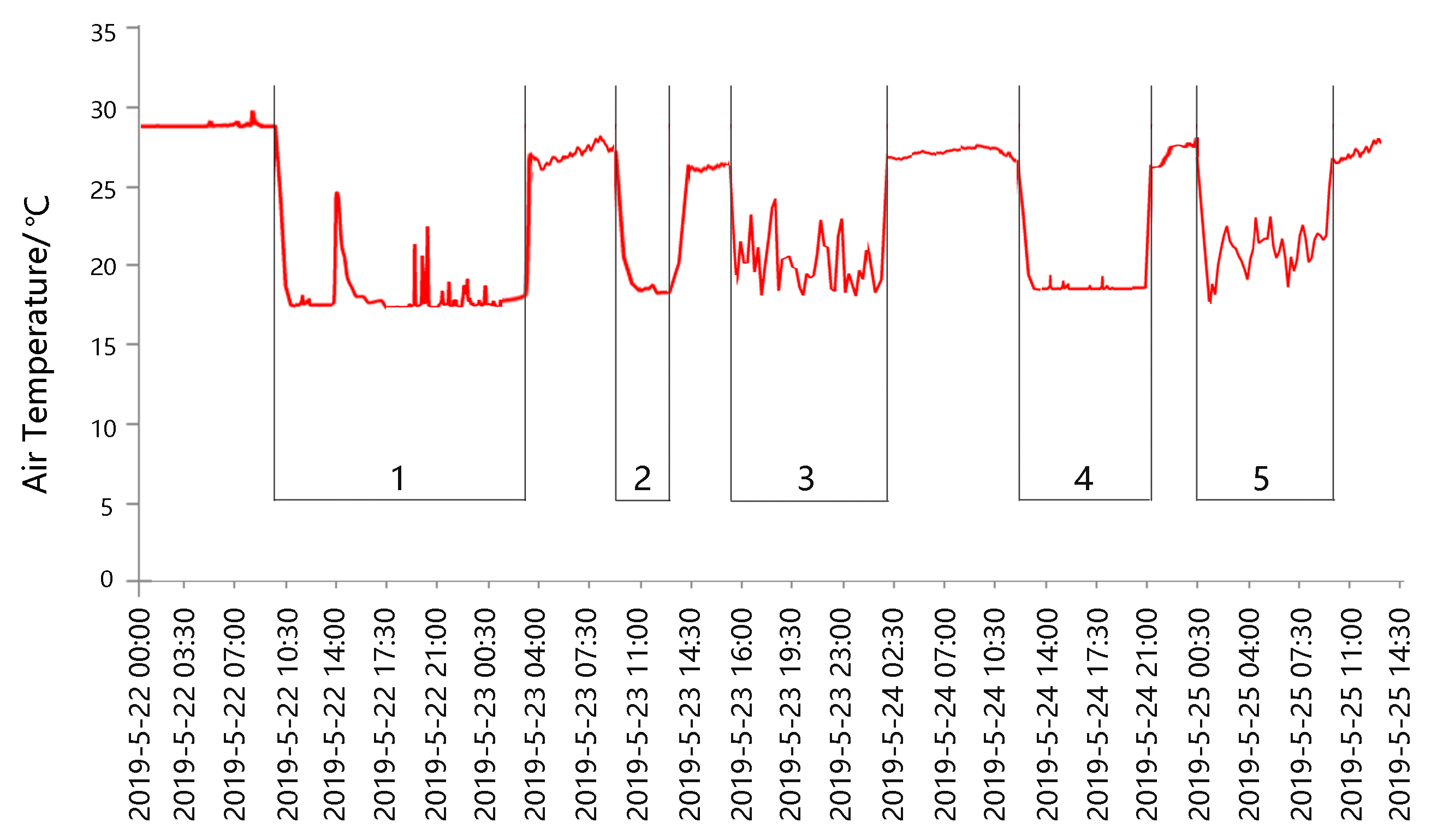
3.1. Data Acquisition

In order to obtain the usage data of electrical equipment in the office, we build an indoor electrical Internet of Things system (IEIoTS), which can obtain the electrical equipment’s state data and environmental parameters by installing smart sockets, smart switches, temperature and humidity sensors, and electrical parameter detection modules. The architecture of this system is shown in Figure 1.

As can be seen from Figure 1, this system includes electrical equipment, a gateway, and a server from the bottom up. The system was deployed in an office building of Shandong Jianzhu University, and the collected data were stored and managed in units of rooms. The electrical equipment of each room included smart sockets, smart switches, and other electrical equipment. The on-off state data of electrical equipment could be acquired by smart sockets and switches, and temperature data were acquired by temperature and humidity sensors. The gateway was the core equipment of the indoor electrical Internet of Things system, which could not only complete the two way transmission of control instructions and state data, but also complete the protocol conversion, and so on [37]. At the top of the system, there was a cloud server to manage the data in the building and store the effective information from the sensors in each room. The data of electrical equipment was uploaded to the database in the cloud server by the gateway for analysis and storage. The TCP/IP protocol was adopted, which could reliably transmit the data collected in the remote environment to the database in real time.

The dataset used in this paper was generated from the IEIoTS deployed in a laboratory building of Shandong Jianzhu University and an occupant in the office. The on/off state data of three pieces of equipment (water dispenser, desktop computer, and light) and the historical data of environmental parameters in the lab were collected and recorded as the original data. The sampling frequency was 1 sample per minute. The original data of half a year were used in this paper, and the total number of the data was 65,880, during which 98% were used as the training data and the remaining 2% as the test data.

3.2. Data Preprocessing

The preprocessing of the original data mainly included: time interception, removing the zero vector, excluding outliers, data interception, etc. The data preprocessing process is shown in Figure 2.

(1)

Time interception: The data should strictly require daily data starting from 00:00, with one minute as the sampling period and yyyy/m/d h:mm as the time format for date processing. One-thousand-four-hundred-forty records could be obtained in one day. It was necessary to determine whether the data were complete. If there was a missing value, we assigned the previous state.

(2)

Removing the zero vector: Removing the state data of the powered device that was not working for a whole day.

(3)

Excluding outliers: For data outliers that occasionally occurred in the original data, outliers were detected and removed by the Laida algorithm [38].

(4)

Data interception: By analyzing the time period of the equipment action daily, the state data during the device on and off time periods were respectively intercepted.

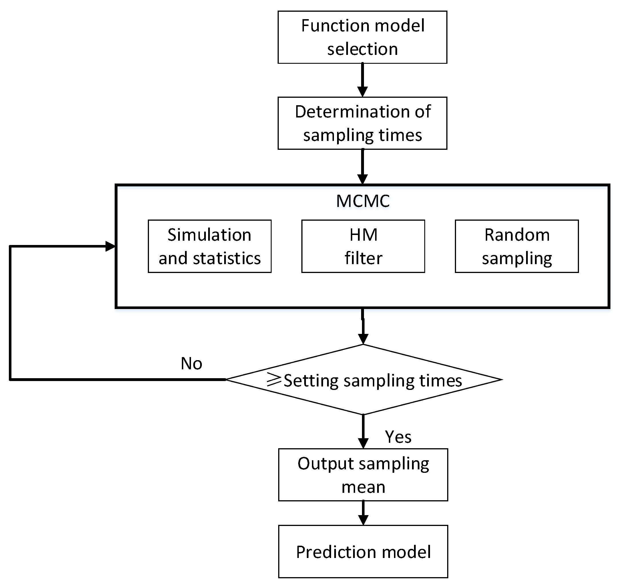
3.3. Model Training

The energy use action model refers to the probability that the electrical equipment enters the power-on and power-off state within a certain temperature; the energy use working hours model refers to the probability of the electrical equipment duration of energy use; and the energy use behavior model of air-conditioner refers to the probability that the air-conditioner enters into the cooling and heating state at a given temperature. Since time and temperature are continuous variables, which are difficult to determine for the entire posterior distribution, the MCMC was used to study the approximate distribution and obtain the fitting curve of the data distribution.

The energy use action model and the energy use working hours model reflect the time rule of user’s energy use behavior. The air-conditioner energy use behavior model reflects user’s thermal comfort, which depends on user’s comfortable temperature range. The process of model training was as follows, taking the energy use action model as an example to elaborate in detail. At first, we needed to observe the electrical equipment’s state distribution based on the time series to determine the fitting function with the parameters that needed to be trained, set the number of samples, and give the initial value to the parameters for the sampling. Secondly, we assumed the a priori distribution of the parameters, and MH random sampling was carried out by searching the distribution space of the parameters. Based on Markov characteristics, new values were randomly assigned to the parameters according to the current state. Thirdly, we checked the new random values; if they satisfied the MH sampling theorem, then we accepted them as a new current state; if not, we rejected and returned them to the previous state. Lastly, we repeated the previous two steps for the specified number of iterations, until it reached the detailed condition of a Markov chain. This method could construct the energy use behavior model based on different time ranges (daily, weekly, annually, etc.), and the calibration frequency of the model needed to be adjusted accordingly. We took the construction of the day based energy use behavior model as an example to evaluate the performance of the proposed method in this paper. The flowchart of energy use behavior prediction is shown in Figure 3.

The algorithm returned all the values generated by the parameters, and the mean of these values was used as the most likely final value for the parameters in the model. We used the Bernoulli function to calculate the probability of the equipment action time. The MCMC returned an approximation of the distribution instead of the accurate results.

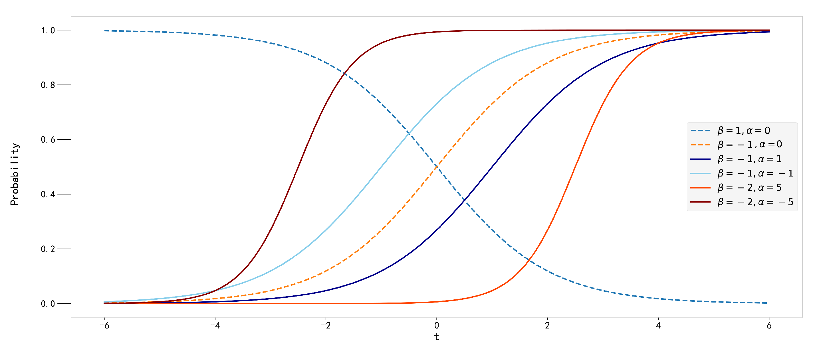
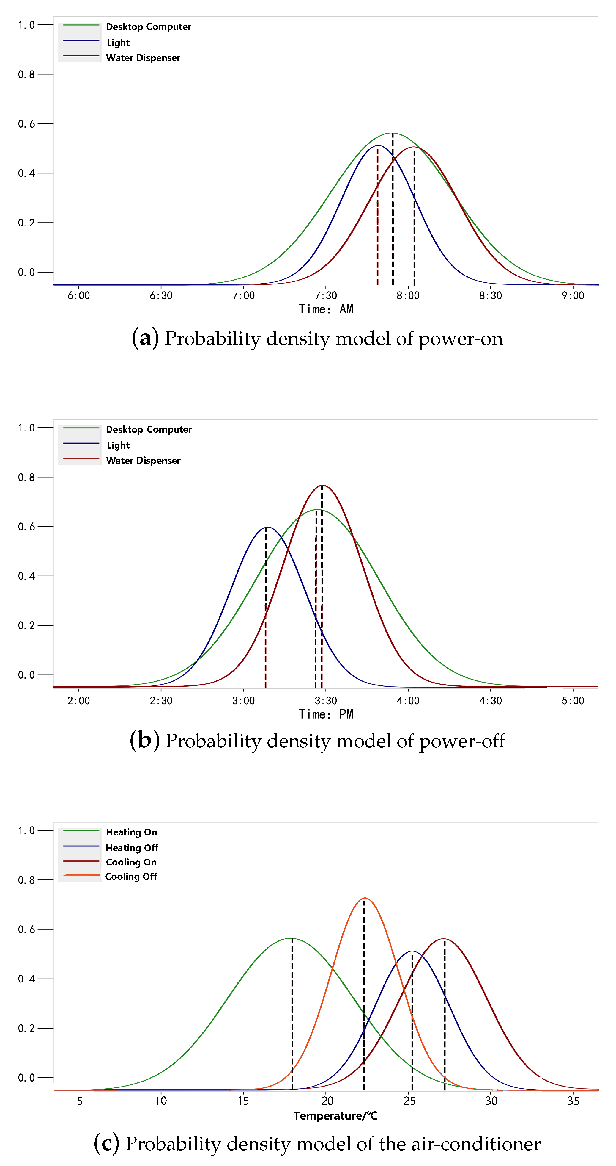
3.3.1. Action Model

(1) Function model selection:

This study took the desktop computer as an example to introduce the algorithm in detail. First, a fitting function was required to model the posterior probability distribution of the energy use action behaviors (on and off) for the desktop computer. The distribution of the historical state data of the desktop computer was observed. The power-on time period was selected as 6:00–9:00, and the power-off time period was selected as 14:00–17:00. The action time probability distribution is shown in Figure 4.

As shown in the Figure 4, it can be concluded that users usually powered on and powered off after 7:30 and 15:00, respectively, and the model was created to simulate the transition process of the user between power-on and power-off in the form of a probability. After many experiments, the logistic function was chosen as the posterior probability distribution model of the on-off action. It can be described as:

$$P\left(action\right|t_i)=\frac{1}{1+e^{\beta t_i+\alpha }}$$

(4)

where t represents the action time. The parameter $\beta$ affects the direction and steepness of the curve; the parameter $\alpha$ affects the position. $\beta$ and $\alpha$ are the two model parameters that need to be trained in the MCMC process jointly. The logistic function with different parameters is shown in Figure 5.

The logistic function satisfied the experimental data, because the probability of the power-on and power-off of the desktop computer would gradually change, which could reflect the change of the on-off action model.

(2) MH sampling:

The procedure of the MH algorithm was randomly sampling from the probability distribution model of the parameters. Each time, the sampling values of the parameters ($\beta$ and $\alpha$) of the function were changed, and the response was observed. The mean value of all sample values was taken to obtain the optimal approximation.

First, in order to plot the random values of the parameters $\beta$ and $\alpha$, it was necessary to assume the prior distribution of the parameters. In this paper, a 2D Gaussian distribution was selected as the prior distribution of the parameters. The two edge distributions of the 2D Gaussian distribution were all in the form of a univariate Gaussian distribution, and this can be expressed as:

$$f\left(x\left|\mu ,\tau \right.\right)=\sqrt{\frac{\tau }{2\pi }}exp\left(-\frac{\tau }{2}{\left(x-\mu \right)}^2\right)$$

(5)

where $\mu$ is the mean of the normal distribution; $\tau$ is the accuracy; $f\left(x\right)$ is Gaussian distribution function. The accuracy ($\tau$) determines the concentration of the distribution; the mean ($\mu$) determines the position of the distribution. The higher the accuracy, the more centralized the presentation data and the smaller the change. The mean can be positive or negative, and the precision must be positive. In order to broaden the search area of the acquired $\beta$ and $\alpha$ values, choose $\mu =0$ and $\tau =0.01$. The parameter space of the prior distribution is shown in Figure 6.

It can be seen from Figure 6 that not every point in the parameter distribution space could be attempted, but the most fitting model could be created by random sampling from a higher probability region (the red part in Figure 6). In order to make the test results more accurate, a step size as long as possible should be chosen. In this paper, the step size was 5000. The MH algorithm evaluated the random values of $\beta$ and $\alpha$ each time. If the MH sampling condition was satisfied, the current values of $\beta$ and $\alpha$ would be accepted, and the state was transferred. If not, the values of $\beta$ and $\alpha$ were random values of the previous time. The sampling trajectory of the parameters $\beta$ and $\alpha$ of the desktop computer power-on model are shown in Figure 7.

The Bernoulli variable was adopted to model the on or off action of equipment, where the power-on was set to 1 and the power-off was set to 0 [39]. The Bernoulli variable of the desktop computer state data depended on the time, which could be defined by the logistic function. It can be described as:

$$S_i\sim Ber\left(p\left(t_i\right)\right),i=1,\cdots ,N$$

(6)

where $p\left(t_i\right)$ is the logistic function with time as the argument, representing the probability of action at a certain time. Therefore, the probability of power-on and power-off was converted by Equation (4), and it can be written in the form:

$$P\left(action\left|t_i\right.\right)=Ber\left(\frac{1}{1+e^{\left(\beta t_i+\alpha \right)}}\right)$$

(7)

The goal of MCMC was to find the optimal values of parameters $\beta$ and $\alpha$ based on the data from the assumption of normal prior distribution. In order to find the most optimal posterior probability distribution of the turn-on and turn-off action model, the mean values of $\beta$ and $\alpha$ samples were taken as the optimal parameters of desktop computer, water dispenser, and light. The probability distribution of the energy use action model is shown in Figure 8.

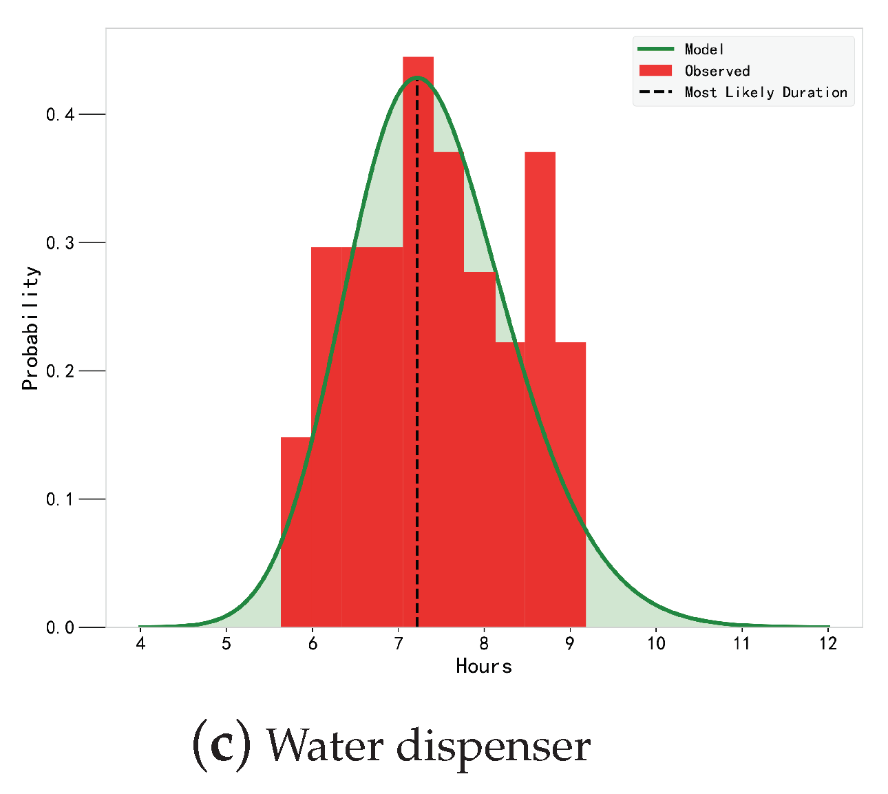
3.3.2. Working Hours Model

According to the characteristics of the data distribution, we adopted the skewed distribution as a posterior distribution of the working hours model. The skewed distribution is the frequency distribution of deviating from the symmetrical value of variables, which can be expressed as:

$$f\left(x;\mu ,\sigma ,\lambda \right)=\frac{2}{\sigma }\varphi \left(\frac{x-\mu }{\sigma }\right)\mathsf{\Phi }\left(\frac{\lambda \left(x-\mu \right)}{\sigma }\right)$$

(8)

where $\varphi (x;\mu ,\sigma )$ and $\mathsf{\Phi }(x;\mu ,\sigma )$ are the density function and distribution function of the standard normal distribution, respectively [40,41]. The MCMC method was used to obtain the optimal values of the mean values $\mu$, variance ${\sigma }^2$, and skewness $\lambda$ in the skewed normal distribution, as well as fitting the maximum probability value of the user electrical equipment’s used time. The energy use working hours models of the desktop computer, light, and water dispenser were established, which are shown in Figure 9.

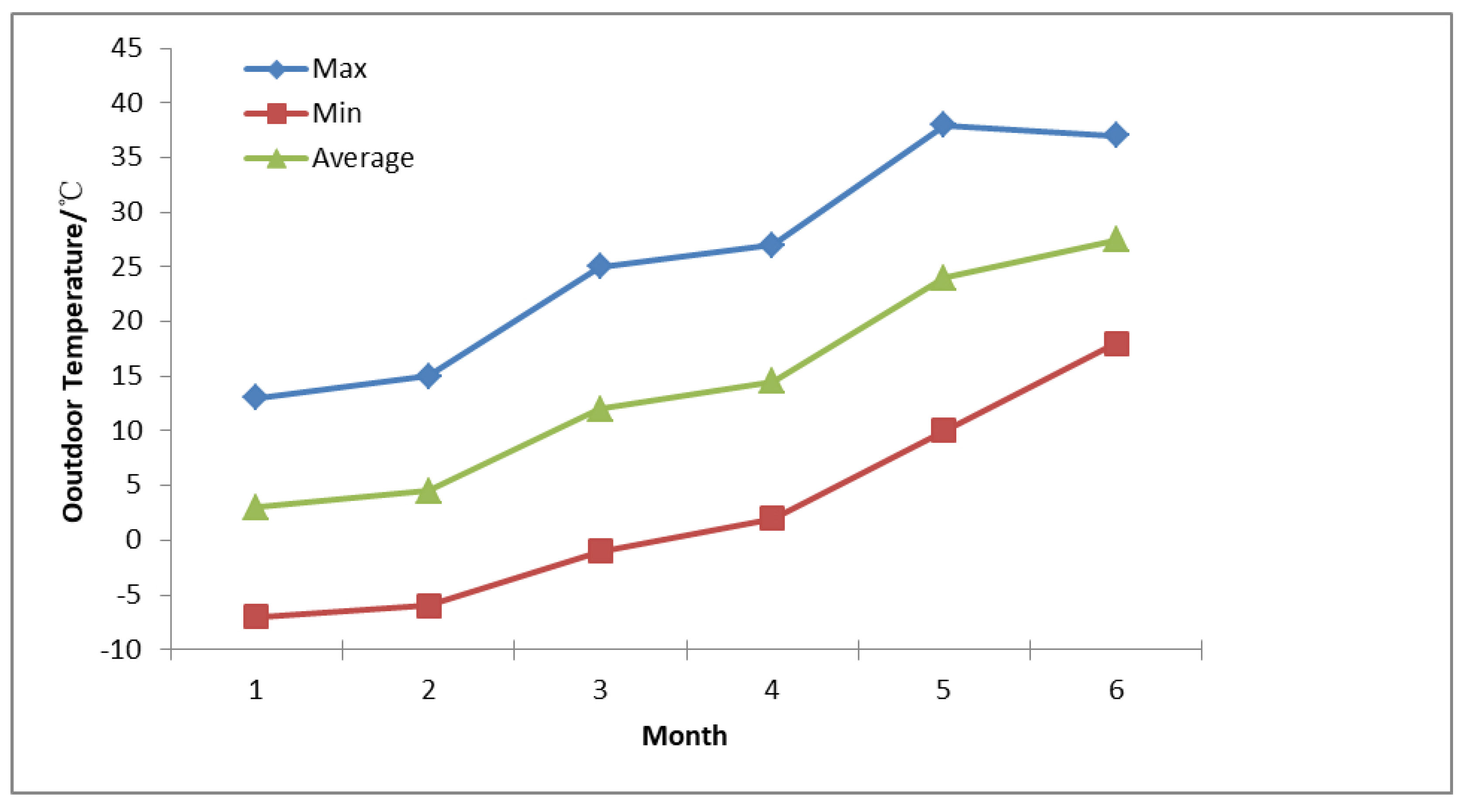
3.3.3. Air-Conditioner Energy Use Behavior Model

The air-conditioner can effectively improve the indoor thermal environment and meet the desired thermal comfort of office occupants. Through the collection of the environmental parameters (temperature, humidity) of the office air outlet, the on-off state and the set temperature of the air-conditioner could be analyzed, then the air-conditioner energy use behaviors of office occupants could be predicted.

The MCMC algorithm was used to build the energy use behavior model of the manual on and off air-conditioner and predict the user’s air-conditioner use behavior based on temperature data. The energy use behavior model of the air-conditioner refers to the probability that the air-conditioner enters into the cooling or heating state in a given temperature. The air-conditioner energy use behavior model included air-conditioner heating-on, heating-off, cooling-on, and cooling-off action model. The training process of the air-conditioner energy use behavior model was similar to the example of the energy use action model in Section 3.3.1. The difference was that the air-conditioner energy use behavior model was based on temperature, while the energy use action model was based on time series of the equipment state. Specifically, the steps of MCMC algorithm for the air-conditioner energy use behavior model are as follows. At first, we needed to observe the air-conditioner state distribution based on the temperature to determine the fitting function with the parameters that needed to be trained; the logistic function was selected similarly, and we set the number of samples and gave the initial value to the parameters for the sampling. Secondly, we assumed the a priori distribution of the parameters was 2D Gaussian, and MH random sampling was carried out by searching the distribution space of the parameters. Based on Markov characteristics, new values were randomly assigned to the parameters according to the current state. Thirdly, we checked the new random values; if they satisfied the MH sampling theorem, then we accepted them as a new current state; if not, we rejected and returned them to the previous state. Lastly, we repeated the previous two steps for the specified number of iterations, until it reached the detailed condition of a Markov chain, which was the probability distributions of the air-conditioner energy use behavior.

The experimental period was from 22 January 2019 to 4 June 2019. The highest, lowest, and average outdoor temperatures of Jinan in each month during the experiment are shown in Figure 10. The temperatures in May and June were higher, with the average temperatures of 24 °C and 27.5 °C, respectively. The highest temperature in May was 38 °C; the lowest temperature in January was −7 °C.

Figure 11 shows the temperature change of a user’s office with the air-conditioner from 22 to 25 May 2019. It can be seen from Figure 11 that the temperature of the air outlet was about 10–15 °C, which was lower than the indoor temperature when the air-conditioner was running. Based on this, the working states of the air-conditioner could be judged.

Figure 11 shows several typical air-conditioner operation processes. Processes 2 and 4 show that after the user turned on the air-conditioner, the air outlet temperature dropped to about 17 °C, and with little fluctuation, so the air-conditioner compressor was in constant frequency operation. After the operation of Processes 1, 3, and 5 for a period of time, due to the frequency conversion of the compressor, the temperature was fluctuating continuously. Before the air-conditioner was started manually, the temperature was basically stable and high. Therefore, the above judgment method could distinguish the manual on and off condition of the air-conditioner from the automatic on and off process, so as to obtain the record of the manual on and off condition of the air-conditioner. Through the above MCMC algorithm, we could get the probability model of the on and off condition of the air-conditioner at a certain temperature, as shown in Figure 12c.

4. Experimental Evaluation

4.1. Evaluation Indices

The root mean squared error (RMSE) and mean absolute error (MAE) are usually used as the loss function of linear regression in machine learning. RMSE is the square root of the squared sum of the deviation between the observed value and the true value with the ratio of the observed times and is used to measure the deviation between the observed value and the true value. MAE is the average of absolute errors, which can better reflect the actual situation of the predicted value error. Therefore, RMSE and MAE were selected to verify the accuracy of the experiment, which can be described as:

$$RMSE=\sqrt{\frac{1}{m}{\sum }_{n=1}^m{\left(\widehat{y_i}-y_i\right)}^2}$$

(9)

$$MAE=\frac{1}{m}{\sum }_{n=1}^m\left|\widehat{y_i}-y_i\right|$$

(10)

where m is the number of sample data; $y_i$ is the true value; $\widehat{y_i}$ represents the predicted value. $y_i$ and $\widehat{y_i}$ are both probability values, and the range is [0,1].

Using the above evaluation indices, the loss between the energy use action time model and the real value of each electrical equipment could be obtained, and the accuracy of the experiment could be evaluated. The MCMC method was used to obtain 5000 sample values, and the average of all sample values was taken as the final parameter of the model. The results of RMSE and MAE are shown in

Table 1. Comparisons of three prediction models in the first experiment.

Equipment Action Model	Optimal Parameter		Evaluation Index
	$\mathit{\alpha }$	$\mathit{\beta }$	RMSE	MAE
Desktop computer Power-on	3.2269	−0.0578	0.0823	0.0517
Desktop computer Power-off	−0.8263	0.0331	0.0732	0.0415
Light Power-on	3.3025	−0.0693	0.0536	0.0346
Light Power-off	−0.4510	0.0345	0.0634	0.0238
Water dispenser Power-on	4.3892	−0.0705	0.0815	0.0591
Water dispenser Power-off	−1.0008	0.0362	0.0924	0.0612
Air-conditioner heating-on	2.8954	−0.0873	0.0687	0.0491
Air-conditioner heating-off	3.7358	−0.0492	0.0824	0.0574
Air-conditioner cooling-on	5.1029	−0.0617	0.0635	0.0329
Air-conditioner cooling-off	4.8796	−0.0584	0.0744	0.0482

; the value of RMSE and MAE of the light power-on model was smaller than the desktop computer power-on model, so the light power-on model was more accurate than the desktop computer power-on model.

4.2. Comparison between MCMC Estimation and MLE

The Maximum Likelihood Estimate (MLE) is a statistical method based on the principle of maximum likelihood, which is the application of probability theory in statistics. It provides a way to estimate a model for a given observation. The steps of solving the maximum likelihood estimation value mainly include: writing out the likelihood function $\ell \left(\theta \right)$ at first, taking the logarithm of the likelihood function, and finally, solving the maximum likelihood function estimation value $\widehat{\theta }$. $\ell \left(\theta \right)$ and $\widehat{\theta }$ can be described as:

$$\ell \left(\theta \right)=p(x_1,x_2,\dots ,x_N\left|\theta \right.)=\prod _{i=1}^{N}p\left(x_i\left|\theta \right.\right)$$

(11)

$$\widehat{\theta }=arg\underset{\theta }{max}\prod _{i=1}^{N}p\left(x_i\left|\theta \right.\right)$$

(12)

where $x_1,x_2,\dots ,x_N$ are samples; ℓ is the parameter vector. We compared the MCMC and MLE algorithm for the analysis of the energy use behavior models corresponding to the optimal parameters $\beta$ and $\alpha$. For the convenience of the statistics, the time periods of [6:00–9:00] and [14:00–17:00] were mapped respectively to the numerical interval of [−85,95] and [−60,120]. The comparative analysis results are shown in

Table 2. Comparison results of MLE and MCMC.

Energy Use Model	MLE			MCMC
	$v$	$L$	$d$	$v$	$L$	$d$
Desktop computer power-on	33.2179	[32.4142,34.0216]	1.6074	33.2637	[32.7747,33.7527]	0.9780
Desktop computer power-off	25.7983	[24.6318,26.9648]	2.3330	25.4528	[24.6492,26.2564]	1.6072
Light power-on	28.3459	[26.8734,29.8184]	2.9450	27.1368	[25.9037,28.3366]	2.4329
Light power-on	23.4086	[22.5467,24.2705]	1.7238	23.8457	[23.6375,24.0539]	0.4164
Water dispenser power-on	40.4608	[39.0547,41.8669]	2.8122	39.7638	[38.9513,40.5763]	1.6250
Water dispenser power-on	26.0109	[25.1376,26.8847]	1.7466	26.5534	[25.7375,27.3693]	1.6318
Air-conditioner heating-on	17.9635	[17.0346,18.8924]	1.8578	18.2389	[17.8934,18.5844]	0.6910
Air-conditioner heating-off	26.0184	[24.7342,27.3076]	2.5684	25.7267	[24.8763,26.5771]	1.7008
Air-conditioner cooling-on	27.8423	[26.3756,29.3090]	2.9334	27.5361	[26.9108,28.1614]	1.2506
Air-conditioner cooling-off	23.4861	[22.0785,24.8937]	2.8152	23.3462	[22.7658,23.9216]	1.1608

, for the desktop computer power-on model; the model interval difference (d) fitted by the MLE algorithm and the MCMC algorithm was 1.6074 and 0.9780, respectively. The smaller the d was, the more the data in the confidence interval, and the better the fitting result. Therefore, the MCMC algorithm was better than the MLE algorithm. By comparing the mean (v), the 90% credible interval (L), and the difference of the interval (d) for the model, it could be obtained that while the mean value performed similarly in estimating the energy use model, the proposed method outperformed the Maximum Likelihood Estimation (MLE) algorithm on uncertainty quantification with relatively narrower confidence intervals.

4.3. Experimental Results and Analysis

In order to analyze energy use behavior intuitively, the probability distribution model of energy use behavior in Figure 8 was transformed into the probability density distribution model, as shown in Figure 12a,b.

As can be seen from the Figure 12a,b, the energy use behaviors had a certain regularity. In the morning, the user tended to turn on the light between 7:40 and 7:50 firstly, then turn on the desktop between 7:50 and 8:00, and finally, turn on the water dispenser between 8:00 and 8:10. In the afternoon, the user turned off the light between 15:10 and 15:20 at first, then turned off the desktop and the water dispenser between 15:20 and 15:30 PM. However, the analysis of the office occupant energy use behavior habits had a high time dependence and uncertainty. The energy use behavior of the office occupants can be deduced from

Table 3. Prediction results of energy use behaviors.

	Prediction	On Period	Off Period	On Time	Off Time	Working Hours (h)
Device
Desktop computer		7:50–8:00	15:20–15:30	7:55	15:25	7.18
Light		7:40–7:50	15:10–15:20	7:47	15:13	7.16
Water dispenser		8:00–8:10	15:20–15:30	8:02	15:27	7.20

.

It can be seen from Figure 12c that the average temperature of air-conditioner cooling-on was 27.5 °C, and the average off temperature was 23.3 °C; the average temperature of air-conditioner heating-on was 18.2 °C, and the average off temperature was 25.7 °C. The on and off behavior of the air-conditioner also reflected the thermal comfort of the users. When the indoor temperature in summer exceeded 27.5 °C, the thermal endurance of users exceeded the threshold value, and the air-conditioner was turned on for cooling; when the indoor temperature dropped to 23.3 °C, the users felt cold, and the air-conditioner was turned off at this time. Therefore, 23.3–27.5 °C could be regarded as the comfortable temperature range for the experimenters under the working condition of the air-conditioner in summer.

5. Conclusions

In this paper, a new method for predicting personal energy use behavior was proposed. Based on the data of electrical equipment used by an office occupant for half a year, the prediction of energy use behavior was realized by using the MCMC method. Firstly, the on-off state data of electrical equipment and temperature history data were obtained by building the IEIoTS for office application, and the experimental data were obtained by data preprocessing. Secondly, the sampling parameters were determined by selecting an a priori function model from observation data. Then, the optimal parameters were obtained through continuous sampling with the MH algorithm in MCMC, and the energy use action model, the energy use working hours model, and the air-conditioner energy use behavior model were fitted. Finally, comparative analysis of the experiments verified that the proposed method had high accuracy and stability. The method proposed in this paper was a generic statistical modeling framework. As long as the user behavior had certain statistical patterns, this method could be used for prediction. Therefore, the model could be applied to other types of buildings, such as residential buildings, industrial buildings, and so on.

In some cases, equipment states and performance data may not be available. For example, considering the user’s privacy, we may not be able to access equipment states of residential buildings, but it is possible to infer the working state information of the equipment by using the aggregated data from the household electricity meters, and then, the method in this paper could be used to predict the user behaviors. Although the proposed method could obtain the rules of personal energy use behaviors, it could not predict the energy use behavior rules with a high resolution. In the future study, we will further improve the accuracy of the algorithm, for example by acquiring longer electrical equipment state data. In addition, we will design energy saving strategies on the basis of office occupants’ energy use behaviors.

References

- Tian, C.; Li, C.; Zhang, G.; Lv, Y. Data driven parallel prediction of building energy consumption using generative adversarial nets. Energy Build. 2019, 186, 230–243. [Google Scholar] [CrossRef]
- Ghalehkhondabi, I.; Ardjmand, E.; Weckman, G.R.; Young, W.A. An overview of energy demand forecasting methods published in 2005-2015. Energy Syst. 2017, 8, 411–447. [Google Scholar] [CrossRef]
- Ren, X.; Yan, D.; Wang, C. Air-conditioning usage conditional probability model for residential buildings. Build. Environ. 2014, 81, 172–182. [Google Scholar] [CrossRef]
- Rafsanjani, H.N.; Ahn, C.R.; Alahmad, M. A review of approaches for sensing, understanding, and improving occupancy-related energy-use behaviors in commercial buildings. Energies 2015, 8, 10996–11029. [Google Scholar] [CrossRef]
- Muncaster, J.; Ma, Y. Activity recognition using dynamic Bayesian networks with automatic state selection. In Proceedings of the 2007 IEEE Workshop on Motion and Video Computing (WMVC’07), Austin, TX, USA, 23–24 February 2007; p. 30. [Google Scholar]
- Shin, J.H.; Lee, B.; Park, K.S. Detection of abnormal living patterns for elderly living alone using support vector data description. IEEE Trans. Inf. Technol. Biomed. 2011, 15, 438–448. [Google Scholar] [CrossRef]
- Nam, Y.; Park, J.W. Child activity recognition based on cooperative fusion model of a triaxial accelerometer and a barometric pressure sensor. IEEE J. Biomed. Health Inform. 2013, 17, 420–426. [Google Scholar]
- Melián-Gutiérrez, L.; Zazo, S.; Blanco-Murillo, J.L.; Pérez-Álvarez, I.; García-Rodríguez, A.; Pérez-Díaz, B. Hf spectrum activity prediction model based on hmm for cognitive radio applications. Phys. Commun. 2013, 9, 199–211. [Google Scholar] [CrossRef]
- Singh, D.; Merdivan, E.; Hanke, S.; Kropf, J.; Geist, M.; Holzinger, A. Convolutional and recurrent neural networks for activity recognition in smart environment. In Towards Integrative Machine Learning and Knowledge Extraction; Springer: Cham, Switzerland, 2017; pp. 194–205. [Google Scholar]
- Withanage, K.I.; Lee, I.; Brinkworth, R.; Mackintosh, S.; Thewlis, D. Fall recovery subactivity recognition with rgb-d cameras. IEEE Trans. Ind. Inform. 2016, 12, 2312–2320. [Google Scholar] [CrossRef]
- Zou, H.; Chen, Z.; Jiang, H.; Xie, L.; Spanos, C. Accurate indoor localization and tracking using mobile phone inertial sensors, wifi and ibeacon. In Proceedings of the 2017 IEEE International Symposium on Inertial Sensors and Systems (INERTIAL), Kauai, HI, USA, 27–30 March 2017; pp. 1–4. [Google Scholar]
- Huang, B.; Qi, G.; Yang, X.; Zhao, L.; Zou, H. Exploiting cyclic features of walking for pedestrian dead reckoning with unconstrained smartphones. In Proceedings of the 2016 ACM International Joint Conference on Pervasive and Ubiquitous Computing, Heidelberg, Germany, 12–16 September 2016; pp. 374–385. [Google Scholar]
- van Kasteren, T.; Noulas, A.; Englebienne, G.; Kröse, B. Accurate activity recognition in a home setting. In Proceedings of the 10th International Conference On Ubiquitous Computing, Seoul, Korea, 21–24 September 2008; pp. 1–9. [Google Scholar]
- Singla, G.; Cook, D.J.; Schmitter-Edgecombe, M. Recognizing independent and joint activities among multiple residents in smart environments. J. Ambient. Intell. Humaniz. Comput. 2010, 1, 57–63. [Google Scholar] [CrossRef]
- van Kasteren, T.L.; Englebienne, G.; Krose, B.J. Hierarchical activity recognition using automatically clustered actions. In Proceedings of the International Joint Conference on Ambient Intelligence, Amsterdam, The Netherlands, 16–18 November 2011; pp. 82–91. [Google Scholar]
- Vail, D.L.; Veloso, M.M.; Lafferty, J.D. Conditional random fields for activity recognition. In Proceedings of the 6th International Joint Conference on Autonomous Agents and Multiagent Systems, Honolulu, HI, USA, 14–18 May 2007; p. 235. [Google Scholar]
- Wu, T.-Y.; Lian, C.-C.; Hsu, J.Y.-J. Joint recognition of multiple concurrent activities using factorial conditional random fields. In Proceedings of the 22nd Conference on Artificial Intelligence (AAAI-2007), Vancouver, BC, Canada, 22–26 July 2007. [Google Scholar]
- Chen, R.; Tong, Y. A two-stage method for solving multi-resident activity recognition in smart environments. Entropy 2014, 16, 2184–2203. [Google Scholar] [CrossRef]
- Zhou, X.; Yan, D.; Hong, T.; Ren, X. Data analysis and stochastic modeling of lighting energy use in large office buildings in china. Energy Build. 2015, 86, 275–287. [Google Scholar] [CrossRef]
- Indraganti, M. Behavioural adaptation and the use of environmental controls in summer for thermal comfort in apartments in india. Energy Build. 2010, 42, 1019–1025. [Google Scholar] [CrossRef]
- Indraganti, M. Thermal comfort in apartments in india: Adaptive use of environmental controls and hindrances. Renew. Energy 2011, 36, 1182–1189. [Google Scholar] [CrossRef]
- Wang, C.; Yan, D.; Ren, X. Modeling individual’s light switching behavior to understand lighting energy use of office building. Energy Procedia 2016, 88, 781–787. [Google Scholar] [CrossRef]
- Kumagai, S.; Kishima, S. Building air conditioning model using the room-specific thermal inertia and its implementation as a controller. IEEJ Trans. Electron. Inf. Syst. 2014, 134, 620–633. [Google Scholar]
- Glicksman, L.R.; Taub, S. Thermal and behavioral modeling of occupant-controlled heating, ventilating and air conditioning systems. Energy Build. 1997, 25, 243–249. [Google Scholar] [CrossRef]
- Hadfield, J.D. Mcmc methods for multi-response generalized linear mixed models: the mcmcglmm r package. J. Stat. Softw. 2010, 33, 1–22. [Google Scholar] [CrossRef]
- Robert, C.P.; Casella, G.; Casella, G. Introducing Monte Carlo Methods with R; Springer: New York, NY, USA, 2010; Volume 18. [Google Scholar]
- Li, C.-Y.; Ji, H.-B. A new particle filter with ga-mcmc resampling. In Proceedings of the 2007 International Conference on Wavelet Analysis and Pattern Recognition, Beijing, China, 2–4 November 2007; Volume 1, pp. 146–150. [Google Scholar]
- Mingas, G.; Rahman, F.; Bouganis, C.-S. On optimizing the arithmetic precision of mcmc algorithms. In Proceedings of the 2013 IEEE 21st Annual International Symposium on Field-Programmable Custom Computing Machines, Seattle, WA, USA, 28–30 April 2013; pp. 181–188. [Google Scholar]
- Andrieu, C.; de Freitas, N.; Doucet, A.; Jordan, M.I. An introduction to mcmc for machine learning. Mach. Learn. 2003, 50, 5–43. [Google Scholar] [CrossRef]
- Jernigan, R.W.; Baran, R.H. Testing lumpability in Markov chains. Stat. Probab. Lett. 2003, 64, 17–23. [Google Scholar] [CrossRef]
- Ng, W.; Reilly, J.P.; Kirubarajan, T.; Larocque, J.-R. Wideband array signal processing using mcmc methods. IEEE Trans. Signal Process. 2005, 53, 411–426. [Google Scholar] [CrossRef]
- Dwivedi, R.; Chen, Y.; Wainwright, M.J.; Yu, B. Log-concave sampling: Metropolis-hastings algorithms are fast! arXiv 2018, arXiv:1801.02309. [Google Scholar]
- Roberts, G.O.; Stramer, O. On inference for partially observed nonlinear diffusion models using the metropolis–hastings algorithm. Biometrika 2001, 88, 603–621. [Google Scholar] [CrossRef]
- Chen, P.; Xu, R.-X. Metropolis-hastings adaptive algorithm and its application. Syst. Eng. Theory Pract. 2008, 1, 100–108. [Google Scholar]
- Chen, M.; Wei, F.; Chao, Y.; Li, X. Bayesian statistics and mcmc method-matlab programming for metropolis-hastings (mh) algorithm. J. East China Jiaotong Univ. 2018, 1, 1–8. [Google Scholar]
- Fries, M.; Baum, A.; Wittmann, M.; Lienkamp, M. Derivation of a real-life driving cycle from fleet testing data with the Markov-chain-monte-carlo method. In Proceedings of the 2018 21st International Conference on Intelligent Transportation Systems (ITSC), Maui, HI, USA, 4–7 November 2018; pp. 2550–2555. [Google Scholar]
- Peng, W.; Li, C.; Zhang, G.; Yi, J. Interval type-2 fuzzy logic based transmission power allocation strategy for lifetime maximization of wsns. Eng. Appl. Artif. Intell. 2020, 87, 103269. [Google Scholar] [CrossRef]
- Fu, C.; Zhang, P.; Jiang, J.; Yang, K.; Lv, Z. A Bayesian approach for sleep and wake classification based on dynamic time warping method. Multimed. Tools Appl. 2017, 76, 17765–17784. [Google Scholar] [CrossRef]
- Fernández-Sáez, J.; Zaera, R.; Loya, J.A.; Reddy, J.N. Bending of euler–bernoulli beams using eringen’s integral formulation: a paradox resolved. Int. J. Eng. Sci. 2016, 99, 107–116. [Google Scholar] [CrossRef]
- Mizuseki, K.; Buzsáki, G. Preconfigured, skewed distribution of firing rates in the hippocampus and entorhinal cortex. Cell Rep. 2013, 4, 1010–1021. [Google Scholar] [CrossRef]
- Schneck, A.; Kalle, S.; Pryss, R.; Schlee, W.; Probst, T.; Langguth, B.; Landgrebe, M.; Reichert, M.; Spiliopoulou, M. Studying the potential of multi-target classification to characterize combinations of classes with skewed distribution. In Proceedings of the 2017 IEEE 30th International Symposium on Computer-Based Medical Systems (CBMS), Thessaloniki, Greece, 22–24 June 2017; pp. 630–635. [Google Scholar]