Article

A Comparative Study of Four Metaheuristic Algorithms, AMOSA, MOABC, MSPSO, and NSGA-II for Evacuation Planning

by
Olive Niyomubyeyi
1,2,*,
Tome Eduardo Sicuaio
1,
José Ignacio Díaz González
1,
Petter Pilesjö
1,3 and
Ali Mansourian
1,3
1
Department of Physical Geography and Ecosystem Science, Lund University, SE-221 00 Lund, Sweden
2
Center for Geographic Information Systems and Remote Sensing, College of Science and Technology, University of Rwanda, Kigali 3900, Rwanda
3
Center for Middle Eastern Studies, Lund University, SE-221 00 Lund, Sweden
*
Author to whom correspondence should be addressed.
Algorithms 2020, 13(1), 16; https://doi.org/10.3390/a13010016
Submission received: 26 November 2019 / Revised: 19 December 2019 / Accepted: 26 December 2019 / Published: 3 January 2020

Abstract

:
Evacuation planning is an important activity in disaster management to reduce the effects of disasters on urban communities. It is regarded as a multi-objective optimization problem that involves conflicting spatial objectives and constraints in a decision-making process. Such problems are difficult to solve by traditional methods. However, metaheuristics methods have been shown to be proper solutions. Well-known classical metaheuristic algorithms—such as simulated annealing (SA), artificial bee colony (ABC), standard particle swarm optimization (SPSO), genetic algorithm (GA), and multi-objective versions of them—have been used in the spatial optimization domain. However, few types of research have applied these classical methods, and their performance has not always been well evaluated, specifically not on evacuation planning problems. This research applies the multi-objective versions of four classical metaheuristic algorithms (AMOSA, MOABC, NSGA-II, and MSPSO) on an urban evacuation problem in Rwanda in order to compare the performances of the four algorithms. The performances of the algorithms have been evaluated based on the effectiveness, efficiency, repeatability, and computational time of each algorithm. The results showed that in terms of effectiveness, AMOSA and MOABC achieve good quality solutions that satisfy the objective functions. NSGA-II and MSPSO showed third and fourth-best effectiveness. For efficiency, NSGA-II is the fastest algorithm in terms of execution time and convergence speed followed by AMOSA, MOABC, and MSPSO. AMOSA, MOABC, and MSPSO showed a high level of repeatability compared to NSGA-II. It seems that by modifying MOABC and increasing its effectiveness, it could be a proper algorithm for evacuation planning.

1. Introduction

Natural disasters are threats to human life and the ecosystem in general. Climate changes as well as environmental changes—e.g., deforestation—increase the frequency and intensity of natural disasters such as hurricanes, floods, and landslides [1]. Such extreme catastrophes cause many losses in lives, affect the economy, and leave many damages to the affected area. However, disaster effects can be reduced if the society is prepared and plans—e.g., for evacuation—are in place.
Evacuation is a means to save lives and is incorporated in both preparedness and response phases of disaster operations management [2]. However, evacuation planning is a complex process and more crucial in urban areas due to the high population density and complex urban settlement. A critical challenge in evacuation planning is to find optimum evacuation time and a proper shelter allocation such that they have enough space for evacuees and other basic living requirements. This means that evacuation planning is considered as a complex multi-criteria decision problem with conflicting objectives, constraints, and spatial aspects. Usually, such problems are modeled by multi-objective optimization techniques, which often provide decision-makers with quick responses and reliable solutions to the problem.
Various studies reported the complexity of evacuation planning in disaster operations management (DOM) and proposed techniques to solve them [3,4]. Thus, depending on the type of disaster and according to the aim of emergency planners, evacuation problems have been modeled as network/routing problems [5,6], transportation problems [7,8], or location-allocation problems [9,10,11]. This study considers evacuation planning as a location-allocation problem.
There are two approaches for solving multi-objective optimization evacuation problems: exact methods and metaheuristic methods. The exact methods—such as linear programming, goal programming, mixed-integer programming, and weighted summation—have been widely used for many decades in disaster operations [12,13]. These methods combine the criteria/objectives of a multi-objective optimization problem with a set of weights provided by decision-makers. Doing so, a single-objective optimization model is created and then a conventional mathematical programming algorithm can be used to solve the problem. Cova and Johnson [14] presented a network flow model for lane-based evacuation routing. Mixed-Integer programming was used as a solution method to identify an optimal lane-based evacuation routing plan in a complex road network.
Although these old and traditional methods have been widely used to solve multi-objective optimization problems, they have limitations when applied to real-world problems. For example, these techniques are often extremely time-consuming to solve real-world problems with large dimensions, hardly constrained problems, and multimodal problems. In addition, the final solution is highly influenced by, and biased towards, the initial weights provided by experts at the early stage of the algorithm. To overcome these limitations, researchers have used multi-objective optimization instead of single-objective optimization in order to design and solve evacuation problems. Metaheuristic algorithms have the ability to produce good quality solutions in reasonable computation time, good enough for a practical purpose [15,16]. They are also not biased with the preferences of experts since no initial weighting of criteria is needed. However, not all of these algorithms are efficient, a few algorithms have proved their capacities for solving real-world problems [17,18]. Moreover, each algorithm has its own limitations. Therefore, it is very important to conduct a comparative study of metaheuristic algorithms on a specific real-world problem.
Saeidian et al. [19] compared two metaheuristic algorithms for location-allocation of earthquake relief centers—genetic algorithm (GA) and bees algorithm (BA). Their results show that BA converges faster than GA, while GA is more favorable in terms of repeatability of the algorithm. Also, Saeidian et al. [20] compared particle swarm optimization (PSO) and ant colony optimization (ACO) using different criteria. The study found that PSO outperformed ACO in terms of quality of solutions, better convergence, and consistency. Xu et al. [21] applied a modified particle swarm optimization (PSO) algorithm combined with a simulated annealing (SA) algorithm to derive solutions using the hybrid bi-level model and conventional multi-objective model for shelters location-allocation problems. The hybrid bi-level model was proven to be useful for optimal shelter allocation. As mentioned in the study by Caunhye et al. [22], the multi-objective approaches are less used and more advanced algorithms are needed to solve many problems in DOM including evacuation.
This paper aims to compare the performance of four metaheuristic algorithms extended from the standard algorithms of simulated annealing (archive multi-objective simulated annealing—AMOSA), artificial bee colony (multi-objective artificial bee colony—MOABC), genetic algorithm (non-dominated sorted genetic algorithm-II—NSGA-II), and particle swarm optimization (multi-objective version of standard particle swarm optimization—MSPSO) for evacuation planning. The four algorithms along with geographic information systems (GIS) are used to solve an urban evacuation problem on a study area in the city of Kigali, Rwanda. Their performance is evaluated based on effectiveness, efficiency, consistency, and computational time for each algorithm.
The remainder of this paper is organized as follows: In Section 2 we review the metaheuristic algorithms and give an overview of the tested four algorithms; Section 3 describes the study area and data preparation; Section 4 explains the methodology used in this study; Section 5 presents the results and analysis, and Section 6 concludes the paper and provides future research directions.

2. An Overview of Metaheuristic Algorithms

Multi-objective optimization problems (MOOP) involve more than one objective function that is to be minimized or maximized. An answer to these types of problems is to find a set of solutions that define the best tradeoff between conflicting objectives. In recent decades, there has been a trend in the scientific community to solve MOOPs by using metaheuristic methods over exact methods. A metaheuristic is defined as a procedure or technique designed for finding the approximate solution in a short time (low computation time) [23]. Metaheuristic approaches categorized as population-based metaheuristics are emerged to find optimal solutions through the iterative process of generating a new population through natural selection. According to Fister Jr. et al. [24], evolutionary algorithms or bio-inspired-based and swarm-intelligence-based algorithms are the most interesting and widely used approaches in population-based metaheuristics. GA and its variants represent a group of evolutionary algorithms, while ABC, ACO, and PSO are three approaches grouped in swarm-intelligence-based algorithms. Those four algorithms are commonly used to solve real-world problems [15]. Another category of metaheuristics is physics/chemistry-based algorithms, which mimic certain physical and or chemical phenomena, including for instance electrical charges, temperature changes, and gravity or river systems. Such algorithms solve a problem based on the process of improving a single solution. SA is the commonly used algorithm in this category [25,26]. These five metaheuristic algorithms are all global optimization methods and can solve higher-dimensional problems; they are robust with respect to the complexity of the evaluation of functions. They can easily be adjusted to the problem at hand. On the other hand, although a lot of research has used these algorithms, the question of finding which one is the best suited for a specific problem has not been answered satisfactorily. Furthermore, maintaining the diversity of optimal solutions and premature convergence of solutions to local optima are still crucial to population-based algorithms.
In order to evaluate all categories, this study used the multi-objective version of four approaches, that is NSGA-II to represent evolutionary algorithms, MOABC and MSPSO to represent swarm-intelligence-based, and AMOSA to represent physics/chemistry-based algorithms. A brief review of each approach is discussed in the following.

2.1. Archive Multi-Objective Simulated Annealing Algorithm

Archive multi-objective simulated annealing (AMOSA) is a global optimization algorithm adapted from the process of annealing in metallurgy. Bandyopadhyay et al. [27] proposed the AMOSA algorithm based on the principle of the original Simulated Annealing (SA) algorithm [28]. In AMOSA, the Pareto dominance approach is adopted and uses the concept of an archive to store all non-dominated solutions. The archive size is limited with two parameters known as hard limit (HL) and soft limit (SL). The HL is the maximum size of the archive on termination, and it is equal to the number of non-dominated solutions required by the user; while SL is the maximum size to which the archive may be filled before clustering is used. The algorithm starts with the set of solutions randomly initialized and refined in the archive by using a hill-climbing technique. A solution is added in the archive if it dominates the previous one and exceeds the HL. If the archive reaches the SL size, then the well-known single-linkage clustering is used to reduce the size of the archive to HL in order to keep a diversity of non-dominated solutions [29]. In the main loop of AMOSA, three cases can occur in dominance:
  • The current solution dominates the new solution and k points from the archive dominate the new solution. In this situation, a new solution can be accepted as the current solution with a given probability.
  • The current solution and the new solution are non-dominating with respect to each other. Here, the domination status of a new solution and members of the archive are checked through three situations: when a new solution is dominated by k points in the archive, the new solution is non-dominating with respect to the points in the archive, and when new solution dominates k points of the archive.
  • The new solution dominates k points of the archive. Here the new solution is selected as the current solution and also added to the archive, while all the k dominated points in the archive are removed. The process in the main loop is repeated through the number of iterations for each temperature, which is reduced to at each iteration using the cooling rate alpha until the minimum temperature is reached. Thereafter, the process stops and the resulting archive contains the final non-dominated solutions.
AMOSA algorithm is capable of solving problems with many objective functions. It has been used to solve medical and engineering-related problems [30,31], but so far there is no literature on AMOSA applied to solve evacuation problems.

2.2. Multi-Objective Artificial Bee Colony Algorithm

Akbari et al. [32] proposed a multi-objective artificial bee colony algorithm (MOABC) based on the standard ABC algorithm developed by Karaboga [33]. Recently, a variant version of MOABC developed based on ABC has been used to solve evacuation problems [34,35]. In this study, the MOABC colony consists of three groups of artificial bees: employed, onlookers, and scout bees. This algorithm generates a number of solutions and works through optimizing them. First, a number of scout bees explore the search space of the problem randomly and generate solutions as the initial population. The quality of the solutions is evaluated (fitness value) and the best solutions are stored in the external memory (archive). The scout bees that have high fitness are selected to act as employed bees. Each employed bee explores the neighborhood to update its position. Onlooker bees select a solution with a high amount of fitness from the neighborhood of employed bees. A new scout bee makes a new generation of the solution if the onlooker failed to update the quality of the solution. Then, the fitness values of all bees are compared to select the best solution and store it to the archive. The Pareto-based approach proposed by Deb et al. [36] has been used to rank the non-dominated solutions into Pareto fronts. The archive is updated by non-dominated solutions, at each iteration. The MOABC algorithm terminates when the termination conditions are met, and the archive returns the final best solutions as output.

2.3. Multi-Objective Standard Particle Swarm Optimization Algorithm

Particle swarm optimization (PSO) is a population-based metaheuristic algorithm introduced by Kennedy and Eberhart [37]. PSO is a swarm intelligence algorithm inspired by the social behavior of bird flocks, fish school. The algorithm has many variants due to its flexibility and robustness in terms of updating the way the velocity of the particle is updated [38,39]. This velocity is the speed of a particle which is used to find its next position in search space. A particle updates its position through topological relationships in the neighborhood. The links between particles facilitate to share information about the previous best position of particles from one to another. PSO has been adapted in many studies related to evacuation planning [40,41,42,43].
In this study, we used the recent standard PSO (SPSO) that was proposed to provide common procedures and guidance to improve the original PSO [44]. However, the proposed SPSO is not for solving complex problems with many objectives. Therefore, we applied a Pareto-based method to evaluate the two objectives simultaneously, and the algorithm is named multi-objective SPSO (MSPSO). MSPSO starts by initializing a random swarm of particles. Each particle is stored in memory with its position, its fitness, and its initial velocity. Then, at each iteration, the velocity of each particle is re-calculated using an equation that contains: (i) the current position of the particle (pbest); (ii) the current velocity; and (iii) the previous best position in the neighborhood (gbest). The fitness is calculated based on new positions of particles found at each iteration. The algorithm can be stopped if a given maximum number of iterations is met.

2.4. Non-Dominated Sorting Genetic Algorithm-II

The NSGA-II algorithm proposed by Deb et al. [36] is the best known multi-objective optimization genetic algorithm and widely used to solve evacuation planning [11,45,46,47]. This algorithm belongs to the class of evolutionary algorithms (EA), in the subclass of genetic algorithms (GA), solving the optimization problem through an evolutional process of the population of individuals.
Initially, a random population P t of size N is initialized, evaluated, and sorted on the basis of non-domination. The fitness of each solution is set to a level number; where level 1 is the best, level 2 is the second-best, and so on. The binary tournament selection, crossover, and mutation operators are applied over P t to generate an offspring population of P t with size N. A solution x i of P t wins a tournament with another solution xj if solution xi has a better rank or if it has the same rank but solution xi has better crowding distance than the solution x j . After generating offspring P t , the main loop of NSGA-II starts by combining the two populations R t = P t + P t and sort R t with the size of 2 N on the basis of non-domination. Then, the elitist selection is applied to select the new population with size N from the highest fronts of R t . This main loop is repeated as many times as needed until the satisfaction of an end criterion (i.e., the number of iterations) is reached. NSGA-II has advantages including its low overall complexity of O ( M N 2 ) .

3. Study Area and Data Description

3.1. Study Area

Kigali is the capital and the most populated city of Rwanda; it accommodates more than 1.135 million inhabitants on an area of 730 km2 [48]. Due to its geographical location and characteristics, many areas of the city are prone to natural disasters such as floods and landslides. In a study by MIDIMAR [49], the hazard-prone areas in Kigali were highlighted based on the frequency of natural hazards, the topography of the area, and the total damages from the experience of disasters. We selected our case study area from one of the hazardous areas (Figure 1).

3.2. Data Description

To start the research process, the first and most important stage is data collection and compilation. At this stage, all required secondary data including spatial and non-spatial were provided by the city of Kigali. Those data are shapefiles of routes, slope, land use, urban villages, and a boundary map along with the needed attribute data such as population. The National Institute Statistics of Rwanda (NISR) provided documents and the population data from the fourth Population and Housing Census of 2012.
Currently, the existing evacuation planning in the city of Kigali does not show a specific place of evacuation. The local authorities are in charge of providing the facilities and locations of safe areas for evacuation and sheltering when a disaster occurs. Thus, the safe areas were selected based on the international standards of evacuation planning for flood and landslide hazards [50]. This includes open spaces, schools, and churches that meet the suitability criteria of being located out of the disaster-prone zones, on gentle slopes and having access to resources, including water sanitation, food, electricity, and toilets.
GIS was used for the preparation and analysis of spatial data. A densely populated region covering an area of 6.9 km2, with a population of 176,741, was selected as a study area (Figure 1b). The population data from NISR was aggregated to the level of small blocks. So, there were 1525 small blocks considered as residential/commercial communities and only one population value was considered for each block. A table was created to store each block, its coordinates, the number of evacuees (population size), and the distance to each shelter following the shortest path. Ten shelters were selected and their capacities were calculated based on the crowd density standard considering 3.5 m2 per person [51]. The table was created to store each candidate shelter, its coordinates, and its capacity to host evacuees. In total, the selected ten shelters have the capacity to host 134,462 evacuated persons. Each shelter might be overloaded due to a large number of evacuees.
A matrix of the shortest distance from each block to each shelter was generated using network analysis in ArcGIS. The origin–destination cost matrix tool was used to compute the minimum distance.

4. Methodology

4.1. Objective Functions for Evacuation Model

As highlighted earlier evacuation planning, in this study, is a location-allocation problem. We adopted two objective functions proposed by Saadatseresht et al. [11]:
  • Function to minimize accumulated distance: This objective function aims at allocating each building block to the nearest shelter.
    f d i s t a n c e = j = 1 n i = 1 m d i j p i j
  • Function to minimize capacity overload: This objective function aims at distributing the overload of the evacuee population among all shelters.
    f c a p a c i t y = j = 1 n | i = 1 m p i j c j 1 |
    where m represents the number of building blocks; n is the number of safe areas, d i j is the distance between the i t h building block and the j t h safe area; p i j is the population in the i t h building block being evacuated to the j t h safe area; and c j is the capacity of the j t h safe area for receiving people.

4.2. Modeling Metaheuristic Algorithms for Evacuation Planning

This section explains the way the allocation of people from the building blocks (residence, commercial, offices) to the safe areas (shelters) is modeled for each of the four algorithms.
The evacuation problem is solved as an unconstrained problem. The discrete method is used to represent the solution for all four algorithms. Figure 2 shows an example of a discrete encoding of the shelter allocation for a study area consisting of 10 building blocks. In Figure 2, a solution is presented as a list; the size of the list corresponds to the number of building blocks. This list contains elements that correspond to the shelters. Since one shelter can accommodate many people from different places, the elements in the list are repeated (many-to-one assignment).

4.2.1. Modeling AMOSA

As mentioned above, the AMOSA algorithm was extended from the principal of simulated annealing to handle multiple objectives problems. This extension lies in determining how to calculate the probability of accepting an individual x where f ( x ) is dominated with respect to f ( x ) . The acceptance of new solutions is based on the probability determined by computing the amount of dominance between two solutions a and b as
Δ d o m a , b =   i   =   1 , f i ( a )     f i ( b ) M ( | f i ( a ) f i ( b ) | R i ) ,
where M = number of objectives and R i is the range of the ith objective. A new solution is selected based on the probability computed with the following equation
p q s   =   1 1 +   e ( E ( q , T ) E ( s , T ) ) T ,
where q is the current state and E ( s ,   T ) and E ( q ,   T ) are the corresponding energy values of s and q , respectively [27].
The solutions were generated as demonstrated in Figure 2. Equations (3) and (4) were used to select and sort the non-dominated solutions in the archive. The algorithm stops when the cooling process reaches the predefined low temperature and the maximum number of iterations.

4.2.2. Modeling MOABC

In MOABC, the coding of the population of the bees is equivalent to the coding of the population in Figure 2. At the starting stage of the algorithm, a population of scout bees is initialized and each bee represents a food source as an array with the size corresponding to the number of building blocks and composed of 10 repeated indices of the 10 shelters. Modeling the fitness function in the MOABC algorithm is similar to those in AMOSA, using Equations (1) and (2). After the initialization and evaluation of fitness, the best solutions are stored in an external archive (new list). Since the archive contains the best solutions found so far, then each employed bee x i d would select a solution from the archive randomly to update it and become v i d . The solution is updated through the equations
v i d = x i d + w · r a n d [ 0 , 1 ] ( x i d x k d ) ,
p i = f ( X i ) i = 0 n f ( X i )
where i represents the food source which is going to be updated, k     { 1 ,   2 , ,   b e e } , and d { 1 ,   2 ,   , D } are randomly chosen indexes. The coefficient w is used to control the influence of the food source k in the production of the new food source.
After evaluating the fitness of employee bees and updating the archive with the best solutions, a roulette wheel selection method is performed to select the onlooker bees for the next generation. The roulette wheel method selects an individual based on the probability p i , found by calculating the proportion of individual fitness f ( x i ) in relation to the total fitness of the n population, as shown in Equation (6). Both employed bees and onlooker bees perform the neighborhood search using the expression in Equation (5) [32]. However, this neighborhood search approach is suitable for the continuous problem, and not for the discrete problem. Thus, in this study, we applied a swap method that randomly selects two elements of a solution and interchanges their indexes. Furthermore, a greedy selection method was applied to evaluate the solution with the best value, comparing an existing solution and a new one. By applying this for all employed bees and onlooker bees, a new bee with the best fitness is selected for the next generation. The best solution is stored in the archive at every iteration of the algorithm. Further exploration is carried out by one scout bee that generates a new random solution. The algorithm is terminated when the given termination criterion (maximum iterations) is attained.

4.2.3. Modeling MSPSO

In the MSPSO algorithm used in this research, every possible arrangement of all building blocks to any candidate shelter can be considered as a potential particle in the search space. The MSPSO algorithm looks for a particle location that satisfies the two defined objective functions of evacuation planning. A particle is defined as a solution and initialized randomly (see Figure 2).
However, the SPSO algorithm was designed for continuous spaces and with real numbers, while in our case the space of the problem is discrete. To solve this, a rounded value method was used for mapping a discrete problem space to the continuous space and vice versa. The 10 shelters are randomly attributed to the integer values of 1 to 10. The real values generated from updating the position of particles (movements of particles) are rounded in order to obtain integer values between 1 and 10. Figure 3 shows an example of an initial particle in continuous space transformed into discrete space after updating of a particle position. The fitness function is calculated using Equations (1) and (2) and assigned to each particle. A neighborhood topology (ring topology) is used to determine the global best (gbest) for each particle among its neighbors. The algorithm is terminated by attaining the maximum number of iterations.

4.2.4. Modeling NSGA-II

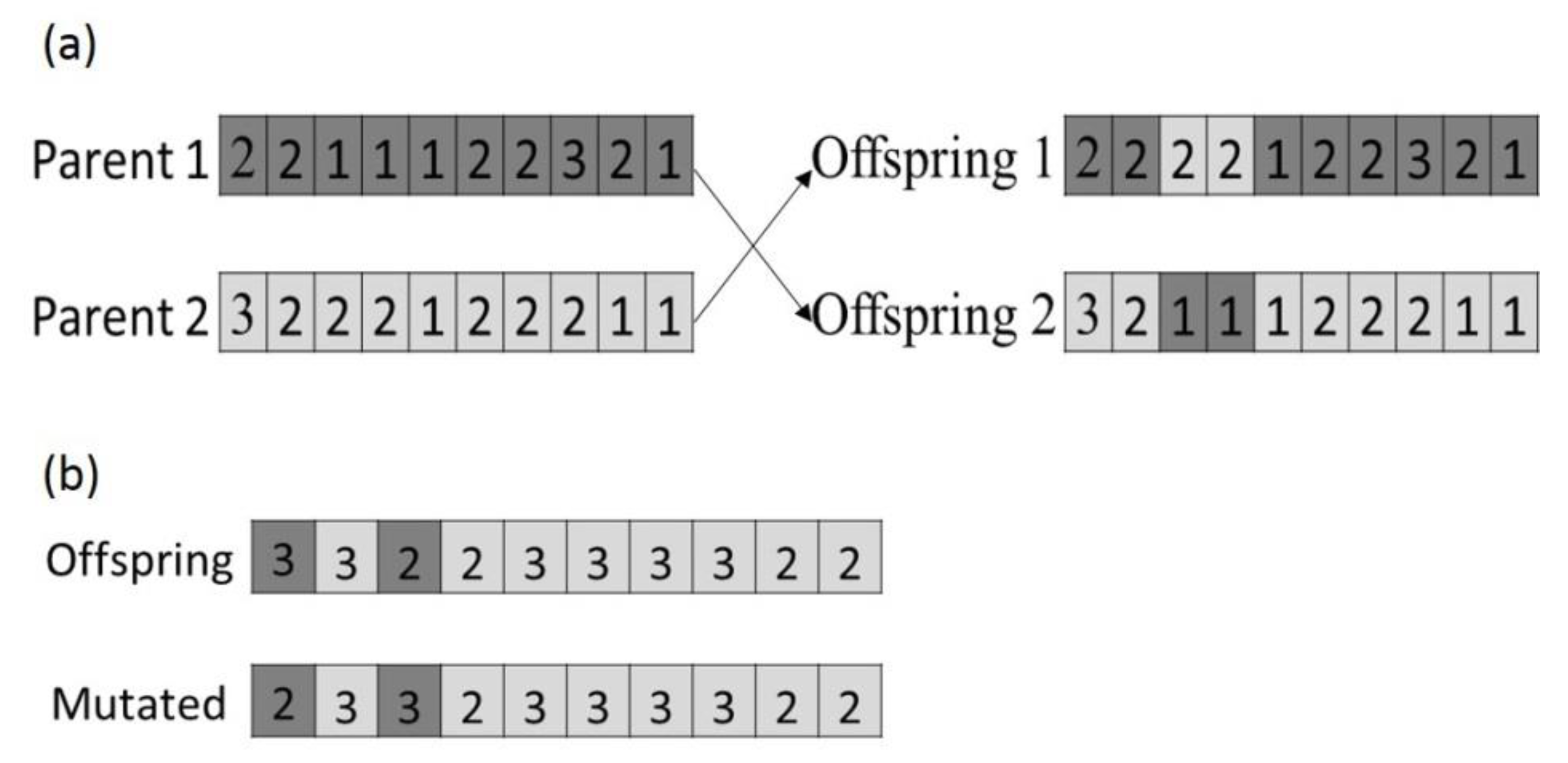
Solving evacuation problem using NSGA-II begins with initializing a population P 0 of chromosomes and then initiate the solutions randomly. The coding of a solution in the form of a chromosome is similar to a solution presented in Figure 2. In this study, the number of genes in each chromosome corresponds to the number of building blocks and each gene contains the index of one shelter with repetition. After initialization, the fitness function is evaluated using Equations (1) and (2). The selection of parent chromosomes of the next generation is done using a tournament selection method based on dominance between two individuals. If the two individuals do not inter-dominate, the selection is made based on crowding distance [52]. This selection technique has also been used by Datta et al. [53] in designing optimal census areas. To generate a new population (offspring), crossover, and mutation operators were applied. The aim of a crossover operator is to exploit the existing best solutions. There are a variety of crossover operators applied in GIS-based genetic procedures [54], and the most used methods include one-point, two-points, and uniform crossover random operators. Here we used the two-point method. This method randomly selects two crossover points and then swaps the vectors of both parents between the two positions as shown in Figure 4a. The two-point crossover has been applied in [55] for optimizing land use planning.
A mutation operator is used to maintain the diversity from one generation to the next and to prevent the issue of local optimum. Two elements of a chromosome are randomly selected and swapped as showed in Figure 4b. After crossover and mutation operations, the elitism strategy is applied to sort the combined population of parents and offspring using the non-dominated sorting method [36].

4.3. Comparing and Evaluating the Performances of Algorithms

In this research, the goal of optimization is to find the best combination of building blocks assigned to shelters, with minimum accumulated distance from building blocks to shelters and minimum overload capacity of all shelters. It is assumed that all building blocks will be assigned a safe area.
To evaluate and compare the four algorithms for the given evacuation problem, the different criteria effectiveness, efficiency (convergence trend, execution time), and repeatability were used. The statistical analysis of variance method (Kruskal–Wallis test) [56] was used to allow us to test how each algorithm achieves the best results and to evaluate if there are statistically significant differences between the tested algorithms. The results from the Kruskal–Wallis (KW) test return the Chi-square value and p-value. A high Chi-square indicates the statistical significance of differences, while the p-value determines if the tested hypothesis should be retained or rejected. If the corresponding KW null hypothesis is rejected, the pairwise comparison is done using the Conover-Iman test [57,58].
The effectiveness of the optimization consists of how good the results of each algorithm is. This study compares the effectiveness of four algorithms for evacuation planning to see how each algorithm minimized the two objective functions: the smaller fitness function value, the better performance in terms of effectiveness criteria.
The convergence trend criteria allowed us to evaluate the fitness variation of the algorithm and get information about the speed of the algorithm needed to reach the optimum solution. Execution time helps to evaluate the computational complexity of the algorithm. Since metaheuristic algorithms use randomness to generate initial solutions and to explore search space of feasible solutions, their results are always different from multiple runs. Considering this, to test the repeatability, we run each algorithm thirty times with the same parameters in order to assess their repeatability.

5. Results of Comparing Algorithms

To compare the performances of the algorithms, we measured and compared four criteria: effectiveness (solution quality), efficiency (convergence speed and execution time), and repeatability.

5.1. Parameter Configuration

Initially, each algorithm has a set of parameters that defines the way they perform the optimization. However, to test these parameters is out of the scope of this research and therefore their values were based on the literature. Nonetheless, since each algorithm works in a different way, several pre-runs were executed in order to look for comparable conditions for them. From this exercise, it was noticed that the parameters population size and maximum number of iterations have significant impact on the results and computation time. Therefore, in order to compare the criteria of effectiveness and efficiency, all algorithms were run on an equal number of the population size of 100 and iterated 500. Other parameters were selected based on the original literature of the algorithms [27,32,36,44]. The tested parameters and their initial values are shown in Table 1.
As highlighted in the study by [59], we recommend future studies to further investigate the parameter tuning of the tested algorithms in this study. Parameter tuning analysis aims to obtain the best parameter setting for each algorithm. Also, note that trial and errors along with the experience of the researchers in understanding how these parameter values correlate to the real-world problem being solved are crucial to achieving satisfactory results.

5.2. Effectiveness Comparison

This study compares the effectiveness of the four algorithms to see how effective each algorithm optimizes the two defined objective functions. Table A1 shows the average and worst fitness values for both capacity and distance functions (fcapacity, fdistance), as well as the execution times obtained for 30 runs of each algorithm. In all 30 cases, AMOSA was the best one optimizing both objective functions, while MSPSO derived extreme values compare to MOABC and NSGA-II. As shown in Table 2, the Kruskal–Wallis test provided very strong evidence of a difference between the mean ranks of the four methods, optimizing the fcapacity and fdistance. The p-values of both functions are smaller than alpha = 0.05. This means that all algorithms perform differently in terms of optimizing the two objective functions.
For effectiveness evaluation in Table 2, the results from the Kruskal-Wallis test shows very strong evidence of a difference (p = 0.000 and p = 0.000) between the mean ranks of the four algorithms in both optimizing fcapacity and fdistance. As shown in Table 3, the pairwise comparison using the Conover-Iman test was carried out to compare the four algorithms and we notice strong evidence of the difference between MSPSO and the other three algorithms, regarding the minimum fitness of capacity as well as distance functions. The asterisk symbol in Table 3 shows where the p-value is less than alpha (α = 0.05), indicating a significant difference between a pair of algorithms in terms of the quality of solutions obtained (see Table A1).
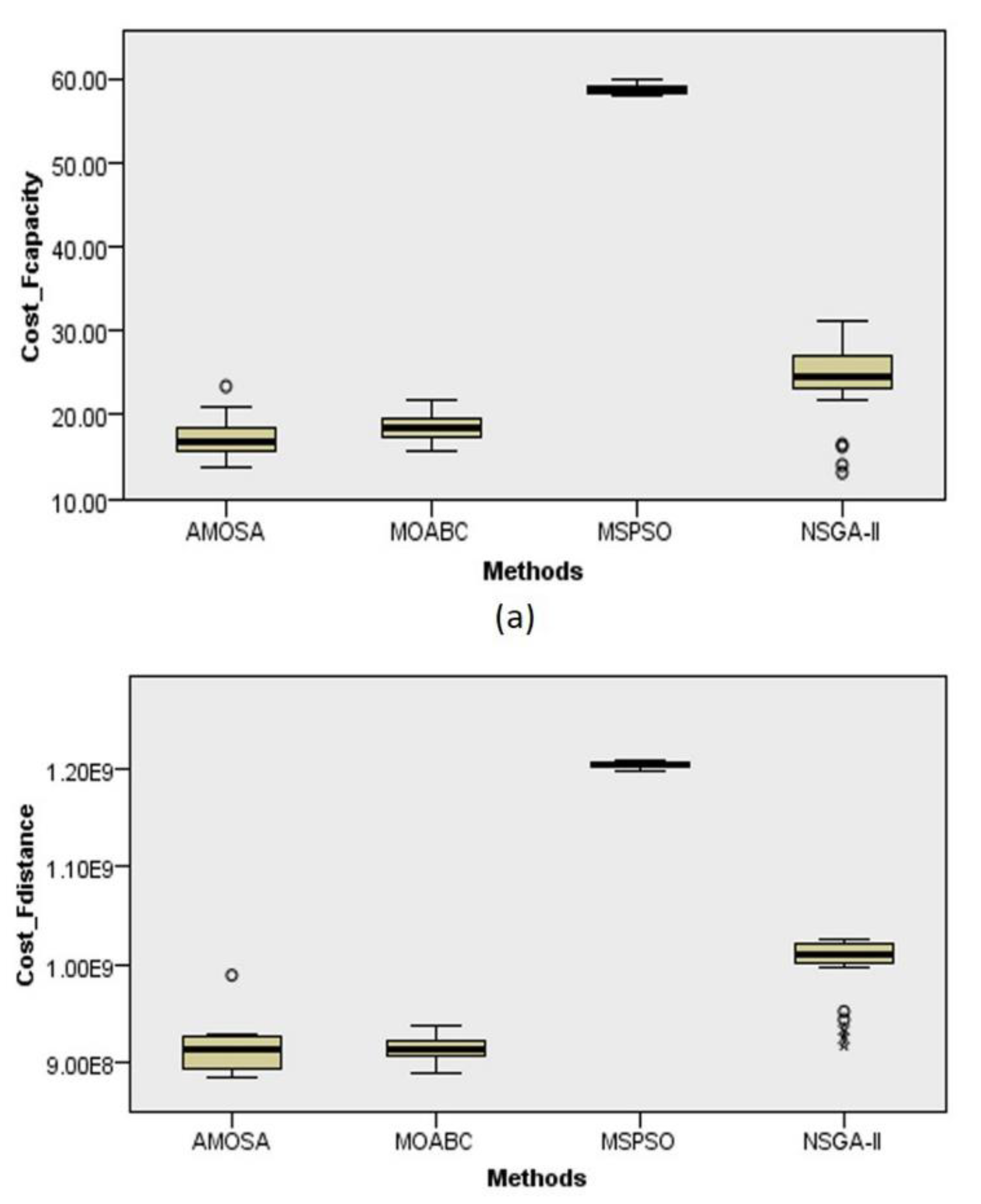
The box plot presents the average cost of two objectives for the four algorithms (Figure 5). Figure 5a,b show that AMOSA and MOABC are the algorithms with the minimum average cost for both objectives. NSGA-II is the third in optimizing both objective functions, while MSPSO has a significantly higher average cost.
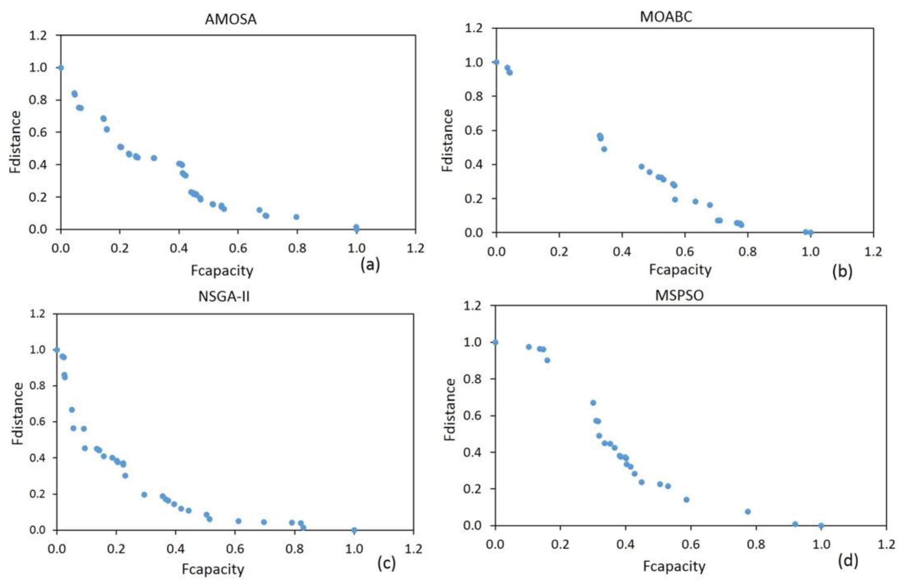
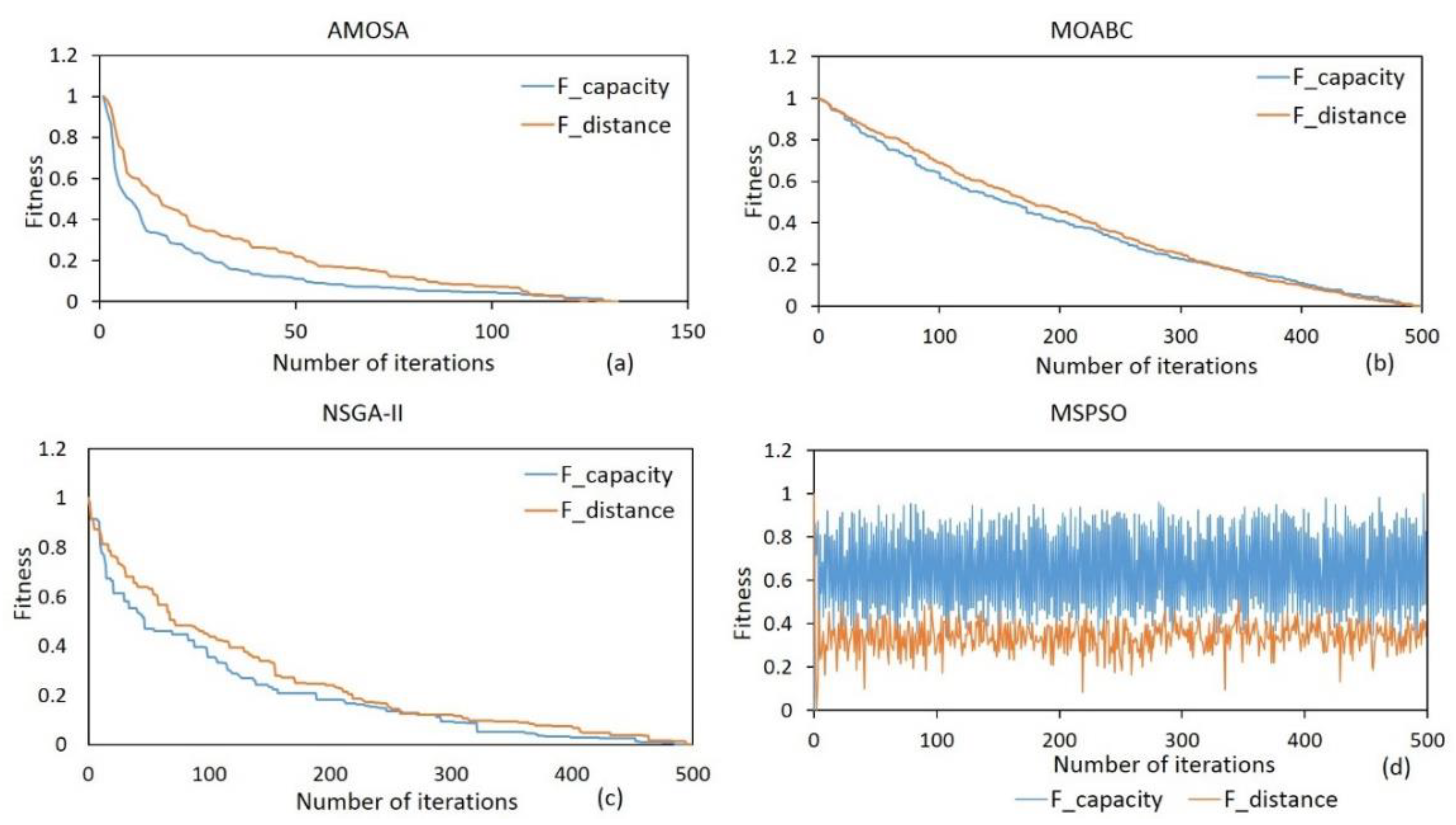
Figure 6 shows that AMOSA returns the high number of solutions while MOABC returns the small number of solutions in the final Pareto front. AMOSA and NSGA-II effectively converge faster to the minimum fitness compare to MOABC and MSPSO. The large size of AMOSA’s solutions is due to its capacity for archiving and clustering solutions that control diversity among the non-dominated solutions. As can be seen in Figure 6, the AMOSA, MSPSO, and NSGA-II show more evenly and smoothly distributed solutions along the Pareto front compared to MOABC.

5.3. Efficiency Comparison

To evaluate the efficiency of the four algorithms in terms of convergence speed and execution time the Kruskal–Wallis test was used. The convergence speed of an algorithm is evaluated based on the fitness variation. This criterion shows how the algorithm converges toward the optimum solution through a number of iterations, while the execution time reveals how fast the algorithm is in terms of running time. The results of the efficiency criteria are presented in Table 2. The p-values in Table 2 show that there is a very significant difference in convergence speed (fitness variation rate) between the algorithms for both objective functions. This is identified by p-value = 0.000, which is less than alpha = 0.05. The post hoc tests using the Conover test were carried out for pairwise convergence comparison, and the results are presented in Table 4. From Table 4, we found that there are statistically significant differences between all algorithms when optimizing the capacity function (p < 0.05). Regarding fitness variation of distance function, only two paired comparisons of MOABC-MSPSO and AMOSA-NSGA-II did not show significant differences (p > 0.05) among six paired comparisons.
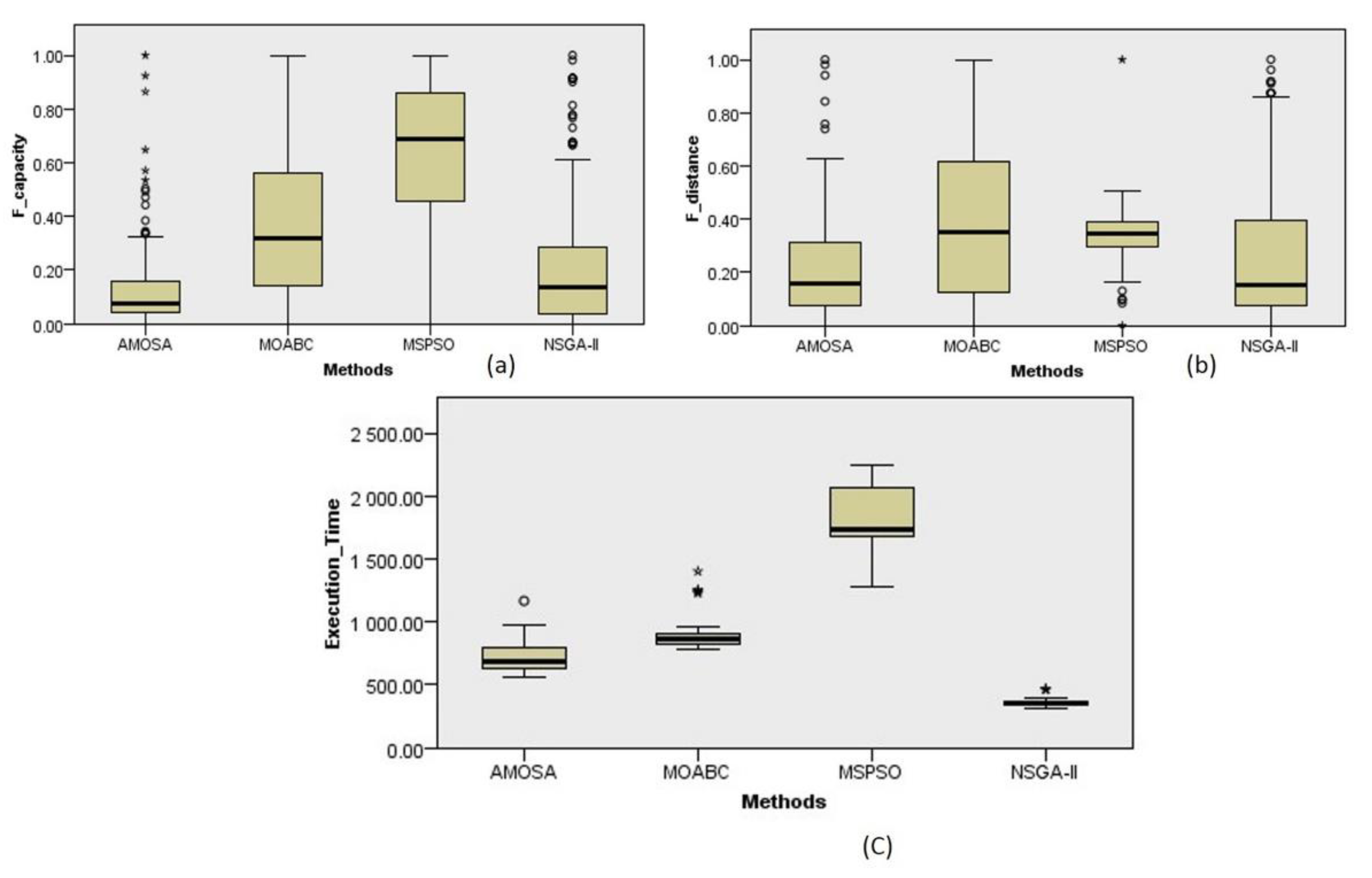
Figure 7 shows a boxplot of fitness variation of both objectives and average execution time for the four algorithms. By assessing box plot a and b in Figure 7, we notice that AMOSA outperforms the other three algorithms, with a minimum average cost for both capacity and distance functions. However, Figure 7c demonstrates that NSGA-II is the fastest algorithm compared to the three others. This shows that the algorithm with high convergence speed is not always the one with the shortest execution time. The execution time is mostly influenced by the size of the population and the number of iterations. For AMOSA, 500 iterations have increased the computation time compared with when the algorithm runs of 100 iterations.
Figure 8 presents the convergence trends of the four algorithms, for both capacity and distance objective functions. The best fitness values of the two functions were normalized in order to facilitate their comparisons. With the progress of the algorithms, the convergence speed is reduced until the optimal solutions are attained. The mean fitness variation of MSPSO is higher compared to that of AMOSA, NSGA-II, and MOABC as shown in Figure 7a,b. Note that for AMOSA, the number of iterations displayed in Figure 8a did not attain 500 as for other algorithms. This is due to its nested loops that also iterate the cooling rate (from high temperature to lower temperature). To avoid the repetitions of solutions, we only retrieved the minimum fitness value obtained after 500 iterations of every degree of the cooling temperature (set to 100 °C).
In general, the convergence speed of AMOSA and NSGA-II are higher (better) followed by MOABC and MSPSO. The reason for smoother convergence of NSGA-II is the crossover and mutation operators that influence to obtain the best survivors (offspring) for the next generation. In contrast with that, the neighborhood search strategy in MSPSO does not guarantee a better improvement of the solutions through iterations. The common challenge of this strategy is to deal with local optimums problem.

5.4. Repeatability Test and Evaluation

A good optimization algorithm is supposed to generate similar results for different runs with the same input parameters. In this section, the repeatability and stability of each algorithm are investigated using the variance of average-normalized fitness values and the average execution time. Each algorithm was implemented five times with the same input data and their results are presented in Table 5.
The four algorithms are different regarding repeatability. As shown in Table 5, NSGA-II has the lowest average execution time of 30 runs, followed by AMOSA and MOABC, and then MSPSO. AMOSA, MOABC, and MSPSO have the lowest average-normalized fitness values for both capacity and distance functions. This indicates that in terms of quality of solutions and repeatability, MOABC and AMOSA are to prefer solving evacuation problems.
The box plot in Figure 7c shows that the average execution time of NSGA-II is 363.03, which is less than half the value of MOABC, and less than a third of MSPSO. Although MOABC and MSPSO are both swarm intelligence algorithms, MOABC outperforms MSPSO. The reason for this difference can be related to the time-consuming neighborhood search process by the particles. The main part of the computation is spent on the calculation of neighborhood topology and comparison of local best and global best fitness values of particles. MOABC, on the other hand, performs a quick exploration of scouts and the share of information between employee and onlooker bees.

5.5. Allocation Maps

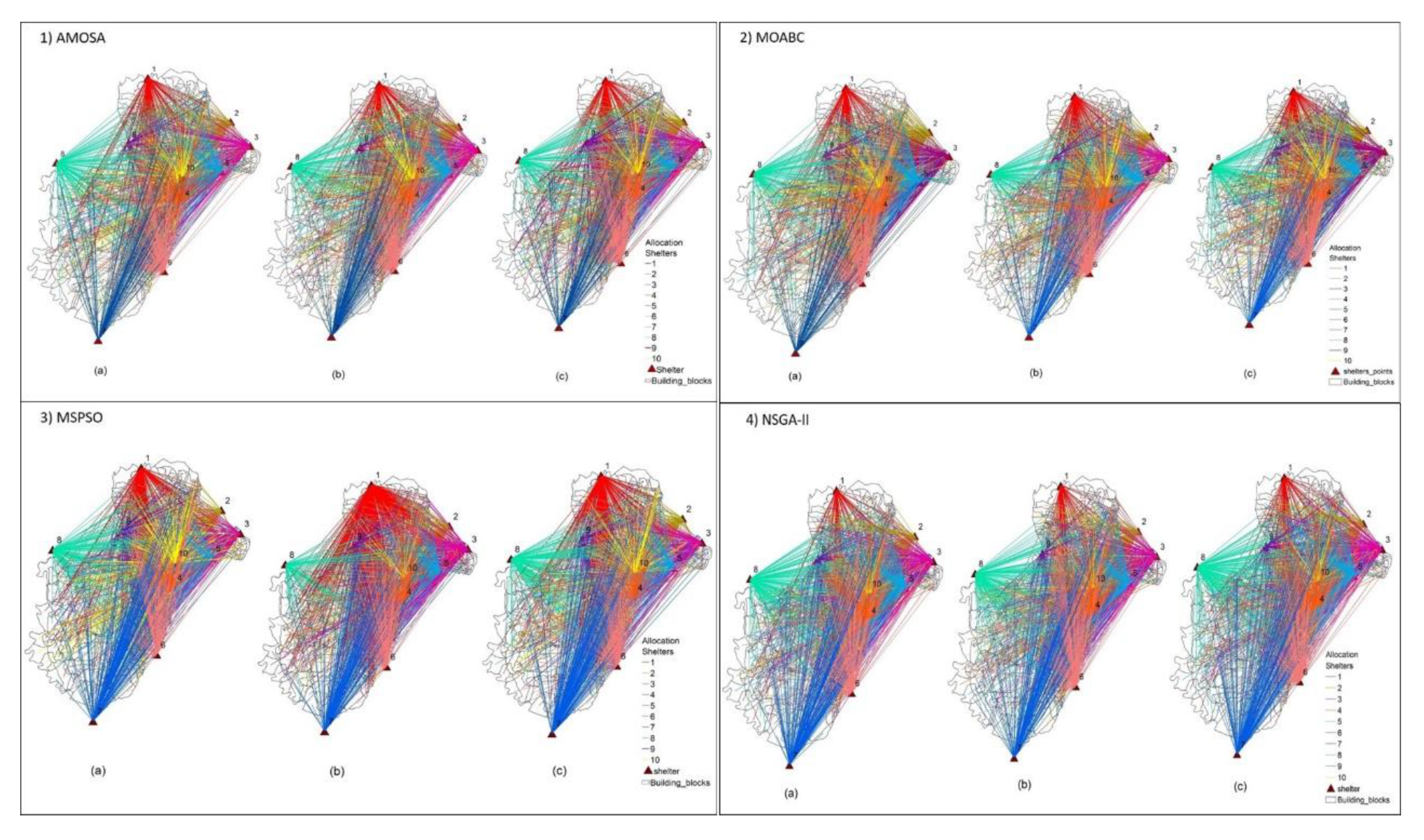
Figure 9 presents the maps of the distribution of the population to shelters as outputs of each algorithm after optimizing the two defined functions. Three solutions are selected from the Pareto front of each algorithm (see Figure 7) by giving higher weight to either minimum objective 1 (Equation (1)) or minimum objective 2 (Equation (2)), or considering the same weight for both objectives. All solutions are optimum and there is a trade-off between them. Meanwhile, decision-makers can select an optimum solution, based on his/her preferences (Figure 9a–c). The lines with different colors represent the allocation of the population from each building block to shelters. The illustrated maps cannot be regarded as an optimal solution for evacuation planning in the city of Kigali. However, decision-makers and planners can use them as input to facilitate the procedure of planning a better distribution of population among the shelters/safe areas. This can be observed in Figure 9 on graphs 1 and 2, where the lines connecting shelters and building blocks look less crowded than graphs 3 and 4.

6. Conclusions

The objective of this study was to compare the performance of four multi-objective optimization algorithms (AMOSA, MOABC, MSPSO, NSGA-II respectively) for a given spatial problem, namely evacuation planning. In our study, the evacuation problem was aiming to minimize the accumulated distance from high-risk zones to shelters and to minimize the total capacity overload cost of shelters. The higher the minimum fitness values of both capacity and distance are, the better are the obtained alternatives for assigning people to appropriate shelters.
In terms of algorithm performance, all algorithms generated the optimization in a consistent way, and no results were obtained that could suggest that some of them were trapped in a local minimum. By evaluating the convergence speed of the fitness variation of the four algorithms (see Figure 8), we found that AMOSA and NSGA-II followed by MOABC converge faster and smoother towards the final optimal solutions. This justifies not only the competence of NSGA-II, which has been used in the literature to a larger extent than the other algorithms [60]. However, the competence of AMOSA and MOABC shows the capacity of solving multi-objective optimization problems including evacuation problems.
The presented metaheuristic methods and others of its type are not meant to find a ‘single perfect solution’ but a set of ‘good enough’ solutions in an efficient way, and therefore, it is possible that a more optimal solution can be achieved by using alternative methods. Decision-makers must be aware of this aspect, in order to properly assess the benefits and limitations of these techniques.
A suggestion for future work, as an alternative approach dealing with this type of spatial multi-objective optimization problems, is to modify the classical algorithms to better fit the problem in hand. For example, based on the results obtained by MOABC and the comparison made to other algorithms, MOABC could be an interesting algorithm to modify in order to solve complex problems such as evacuation planning. It is also important to consider the use of other methods, such as recoverable robustness, to solve evacuation planning. Iris and Lam [61] proposed a recoverable robust optimization approach for the weekly berth and quay crane planning problem. The results proved the strength of the proposed model for solving a spatial problem.

Author Contributions

O.N. was responsible for methodology, implementation, testing and analysis, and writing; T.E.S. contributed in formal analysis and editing; J.I.D.G. contributed in implementation, analysis, and editing; P.P. was responsible for supervision and conceptualization; A.M. was responsible for idea development and conceptualization, coordination, supervision, reconstruction, and editing the manuscript. All authors have read and agreed to the published version of the manuscript.

Funding

This research was funded by the Swedish International Development Agency (SIDA) through the University of Rwanda-Sweden Program, GIS Sub-Program. Grant Agreement between Sweden, the Government of Rwanda and the University of Rwanda (UR) regarding the “University of Rwanda and Sweden Research Partnership 2019-2024” Sida Contribution No 11277.

Acknowledgments

The authors would like to express their thanks to the University of Rwanda, Lund University, and SIDA Partnership Program for their financial support of this research.

Conflicts of Interest

The authors declare no conflicts of interest.

Appendix A

In the results section of this article, only a summarized set of graphs was presented for specific analysis. This appendix contains a table showing the full output of the optimization of each algorithm.
Table A1. The average and worst fitness values of capacity and distance functions, and the execution time of 30 runs for each algorithm.
RunsAverage Minimum FcapacityAverage Minimum FdistanceAMOSA Algorithm Worst FcapacityWorst FdistanceTime(s)Average Minimum FcapacityAverage Minimum FdistanceMOABC Algorithm Worst FcapacityWorst FdistanceTime(s)Average Minimum FcapacityAverage Minimum FdistanceMSPSO Algorithm Worst FcapacityWorst FdistanceTime(s)Average Minimum FcapacityAverage Minimum FdistanceNSGA-II Algorithm Worst FcapacityWorst FdistanceTime(s)
116.139.19 × 10827.009.39 × 10856417.979.28 × 10820.659.85 × 108124858.431.20 × 10970.661.27 × 109209716.499.52 × 10826.531.02 × 109468
217.399.29 × 10823.079.71 × 10867719.769.22 × 10822.919.56 × 108125558.561.21 × 10969.061.27 × 109207614.069.35 × 10818.919.99 × 108462
318.429.14 × 10825.389.66 × 10868019.329.35 × 10822.569.79 × 108140258.881.20 × 10968.601.26 × 109207721.669.44 × 10834.241.03 × 109465
416.479.24 × 10824.609.77 × 10858017.229.27 × 10818.169.74 × 108124158.901.21 × 10970.561.26 × 109206916.269.27 × 10821.961.04 × 109332
516.518.95 × 10821.829.36 × 10860416.979.14 × 10818.109.34 × 108122858.691.21 × 10970.581.25 × 109207013.159.18 × 10821.689.71 × 108329
623.409.89 × 10825.941.00 × 10963020.069.16 × 10823.239.60 × 10888658.721.20 × 10973.441.25 × 109162026.871.02 × 10942.011.12 × 109367
715.568.91 × 10819.779.33 × 108116719.519.10 × 10822.599.77 × 10879758.421.20 × 10971.451.25 × 109162926.611.02 × 10951.041.12 × 109363
818.388.88 × 10827.859.32 × 10861519.989.02 × 10821.879.31 × 10883559.491.21 × 10968.941.26 × 109129626.371.01 × 10940.291.15 × 109353
918.708.99 × 10829.479.39 × 10868216.499.11 × 10817.679.22 × 10884158.351.21 × 10971.811.27 × 109127824.461.02 × 10934.931.13 × 109346
1015.079.30 × 10824.349.85 × 10868919.209.10 × 10820.799.39 × 10882358.401.20 × 10966.921.26 × 109169827.001.01 × 10938.931.08 × 109359
1119.958.88 × 10832.159.19 × 10861020.859.06 × 10824.349.39 × 10878459.151.21 × 10970.251.29 × 109155425.201.01 × 10939.101.08 × 109364
1221.059.28 × 10836.649.93 × 10871818.279.06 × 10820.699.28 × 10878359.001.21 × 10969.641.27 × 109178126.701.03 × 10943.891.11 × 109314
1315.309.22 × 10825.259.69 × 10874317.469.03 × 10819.439.18 × 10881258.961.21 × 10970.711.25 × 109176231.241.00 × 10956.201.09 × 109351
1416.879.25 × 10830.329.84 × 10870518.579.10 × 10821.889.33 × 10878259.761.20 × 10971.311.27 × 109172124.311.01 × 10934.611.13 × 109330
1516.789.17 × 10826.609.70 × 10881917.069.14 × 10820.019.53 × 10880658.791.20 × 10971.521.29 × 109170323.381.00 × 10947.361.06 × 109356
1618.568.87 × 10828.109.37 × 10868317.669.24 × 10821.019.72 × 10895858.781.21 × 10970.761.25 × 109176723.451.03 × 10940.941.11 × 109346
1718.259.09 × 10826.599.86 × 10896317.169.37 × 10819.129.70 × 10879058.261.20 × 10971.091.26 × 109158825.751.03 × 10946.971.14 × 109322
1815.769.12 × 10824.809.84 × 10869719.509.23 × 10824.169.68 × 10887058.071.20 × 10968.301.24 × 109168024.521.03 × 10933.031.12 × 109348
1916.799.18 × 10825.029.71 × 10895619.919.12 × 10822.629.32 × 10891558.131.21 × 10969.771.28 × 109176929.321.00 × 10946.321.08 × 109341
2013.778.94 × 10818.259.31 × 10868915.588.88 × 10816.488.94 × 10888058.271.21 × 10969.301.26 × 109170022.861.01 × 10942.981.09 × 109361
2114.729.11 × 10821.059.42 × 10869318.189.14 × 10821.009.68 × 10886058.261.20 × 10968.441.26 × 109184629.709.97 × 10854.151.07 × 109341
2215.798.85 × 10823.419.40 × 10894818.649.24 × 10821.499.56 × 10886158.051.21 × 10967.601.25 × 109173826.201.02 × 10940.991.13 × 109328
2317.469.26 × 10826.869.78 × 10867918.779.07 × 10823.489.37 × 10886858.611.21 × 10974.471.28 × 109172223.211.02 × 10932.061.11 × 109352
2418.179.09 × 10827.709.65 × 10861117.449.04 × 10819.579.41 × 10889059.001.20 × 10968.601.25 × 109222221.941.03 × 10936.481.13 × 109360
2513.679.16 × 10819.359.51 × 10897220.219.17 × 10823.929.48 × 10889358.581.21 × 10968.091.26 × 109174424.171.02 × 10932.151.19 × 109379
2615.648.90 × 10822.689.19 × 10873319.548.91 × 10821.538.96 × 10886359.011.20 × 10973.621.26 × 109224029.231.02 × 10953.301.12 × 109401
2718.589.28 × 10827.069.95 × 10878818.759.16 × 10822.959.33 × 10885658.401.21 × 10968.961.26 × 109175324.291.00 × 10949.581.08 × 109357
2818.748.92 × 10825.219.35 × 10868517.009.17 × 10817.779.47 × 10889557.831.20 × 10967.631.26 × 109206227.501.01 × 10940.211.09 × 109335
2915.768.94 × 10822.539.28 × 10895718.409.09 × 10820.549.35 × 10890759.011.20 × 10973.871.28 × 109167527.341.01 × 10941.971.09 × 109385
3018.429.28 × 10833.869.70 × 10856321.839.01 × 10825.679.31 × 10883358.331.20 × 10968.491.24 × 109167024.751.01 × 10937.931.08 × 109376

References

  1. Banholzer, S.; Kossin, J.; Donner, S. The Impact of Climate Change on Natural Disasters. In Reducing Disaster: Early Warning Systems for Climate Change; Singh, A., Zommers, Z., Eds.; Springer: Dordrecht, The Netherlands, 2014; pp. 21–49. [Google Scholar]
  2. Perry, R.W.; Lindell, M.K. Preparedness for Emergency Response: Guidelines for the Emergency Planning Process. Disasters 2003, 27, 336–350. [Google Scholar] [CrossRef] [PubMed]
  3. Galindo, G.; Batta, R. Review of recent developments in OR/MS research in disaster operations management. Eur. J. Oper. Res. 2013, 230, 201–211. [Google Scholar] [CrossRef]
  4. Özdamar, L.; Ertem, M.A. Models, solutions and enabling technologies in humanitarian logistics. Eur. J. Oper. Res. 2015, 244, 55–65. [Google Scholar] [CrossRef]
  5. Coutinho-Rodrigues, J.; Tralhão, L.; Alçada-Almeida, L. Solving a location-routing problem with a multiobjective approach: The design of urban evacuation plans. J. Transp. Geogr. 2012, 22, 206–218. [Google Scholar] [CrossRef]
  6. Wu, W.-X.; Huang, H.-J. A combined, adaptive strategy for managing evacuation routes. Transp. Res. Part B Methodol. 2019, 123, 182–198. [Google Scholar] [CrossRef]
  7. Stepanov, A.; Smith, J.M. Multi-objective evacuation routing in transportation networks. Eur. J. Oper. Res. 2009, 198, 435–446. [Google Scholar] [CrossRef]
  8. Murray-Tuite, P.; Wolshon, B. Evacuation transportation modeling: An overview of research, development, and practice. Transp. Res. Part C Emerg. Technol. 2013, 27, 25–45. [Google Scholar] [CrossRef]
  9. Sherali, H.D.; Carter, T.B.; Hobeika, A.G. A location-allocation model and algorithm for evacuation planning under hurricane/flood conditions. Transp. Res. Part B Methodol. 1991, 25, 439–452. [Google Scholar] [CrossRef]
  10. Kongsomsaksakul, S.; Yang, C.; Chen, A. Shelter location-allocation model for flood evacuation planning. J. East. Asia Soc. Transp. Stud. 2005, 6, 4237–4252. [Google Scholar]
  11. Saadatseresht, M.; Mansourian, A.; Taleai, M. Evacuation planning using multiobjective evolutionary optimization approach. Eur. J. Oper. Res. 2009, 198, 305–314. [Google Scholar] [CrossRef]
  12. Cohon, J.L. Multiobjective Programming and Planning; Academic Press: Cambridge, MA, USA, 1978. [Google Scholar]
  13. Xie, C. Evacuation Network Optimization: Models, Solution Methods and Applications. Available online: https://ecommons.cornell.edu/handle/1813/10869 (accessed on 29 December 2019).
  14. Cova, T.J.; Johnson, J.P. A network flow model for lane-based evacuation routing. Transp. Res. Part Policy Pract. 2003, 37, 579–604. [Google Scholar] [CrossRef]
  15. Zheng, Y.-J.; Chen, S.-Y.; Ling, H.-F. Evolutionary optimization for disaster relief operations: A survey. Appl. Soft Comput. 2015, 27, 553–566. [Google Scholar] [CrossRef]
  16. Urena Serulle, N.; Cirillo, C. The optimal time to evacuate: A behavioral dynamic model on Louisiana resident data. Transp. Res. Part B Methodol. 2017, 106, 447–463. [Google Scholar] [CrossRef]
  17. Yang, X.-S. Nature-Inspired Optimization Algorithms; Elsevier: Amsterdam, The Netherlands, 2014. [Google Scholar]
  18. Bujok, P.; Tvrdík, J.; Poláková, R. Comparison of nature-inspired population-based algorithms on continuous optimisation problems. Swarm Evol. Comput. 2019, 50, 100490. [Google Scholar] [CrossRef]
  19. Saeidian, B.; Mesgari, M.S.; Ghodousi, M. Evaluation and comparison of Genetic Algorithm and Bees Algorithm for location–allocation of earthquake relief centers. Int. J. Disaster Risk Reduct. 2016, 15, 94–107. [Google Scholar] [CrossRef]
  20. Saeidian, B.; Mesgari, M.S.; Pradhan, B.; Ghodousi, M. Optimized Location-Allocation of Earthquake Relief Centers Using PSO and ACO, Complemented by GIS, Clustering, and TOPSIS. ISPRS Int. J. Geo-Inf. 2018, 7, 292. [Google Scholar] [CrossRef] [Green Version]
  21. Xu, W.; Ma, Y.; Zhao, X.; Li, Y.; Qin, L.; Du, J. A comparison of scenario-based hybrid bilevel and multi-objective location-allocation models for earthquake emergency shelters: A case study in the central area of Beijing, China. Int. J. Geogr. Inf. Sci. 2018, 32, 236–256. [Google Scholar] [CrossRef]
  22. Caunhye, A.M.; Nie, X.; Pokharel, S. Optimization models in emergency logistics: A literature review. Socio-Econ. Plan. Sci. 2012, 46, 4–13. [Google Scholar] [CrossRef]
  23. Talbi, E.G. Metaheuristics: From Design to Implementation; John Wiley & Sons: Hoboken, NJ, USA, 2009. [Google Scholar]
  24. Fister, I., Jr.; Yang, X.-S.; Fister, I.; Brest, J.; Fister, D. A Brief Review of Nature-Inspired Algorithms for Optimization. arXiv 2013, arXiv:1307.4186. [Google Scholar]
  25. Jahangiri, A.; Afandizadeh, S.; Kalantari, N. The optimization of traffic signal timing for emergency evacuation using the simulated annealing algorithm. Transport 2011, 26, 133–140. [Google Scholar] [CrossRef]
  26. Yadollahnejad, V.; Bozorgi-Amiri, A.; Jabalameli, M. Allocation and Vehicle Routing for Evacuation Operations: A Model and a Simulated Annealing Heuristic. J. Urban Plan. Dev. 2017, 143, 04017018. [Google Scholar] [CrossRef]
  27. Bandyopadhyay, S.; Saha, S.; Maulik, U.; Deb, K. A Simulated Annealing-Based Multiobjective Optimization Algorithm: AMOSA. IEEE Trans. Evol. Comput. 2008, 12, 269–283. [Google Scholar] [CrossRef] [Green Version]
  28. Kirkpatrick, S.; Gelatt, C.D.; Vecchi, M.P. Optimization by simulated annealing. Science 1983, 220, 671–680. [Google Scholar] [CrossRef] [PubMed]
  29. Jain, A.K.; Dubes, R.C. Algorithms for Clustering Data; Prentice-Hall, Inc.: Upper Saddle River, NJ, USA, 1988. [Google Scholar]
  30. Acharya, S.; Saha, S.; Thadisina, Y. Multiobjective Simulated Annealing-Based Clustering of Tissue Samples for Cancer Diagnosis. IEEE J. Biomed. Health Inform. 2016, 20, 691–698. [Google Scholar] [CrossRef]
  31. Alok, A.K.; Saha, S.; Ekbal, A. Multi-objective semi-supervised clustering for automatic pixel classification from remote sensing imagery. Soft Comput. 2016, 20, 4733–4751. [Google Scholar] [CrossRef]
  32. Akbari, R.; Hedayatzadeh, R.; Ziarati, K.; Hassanizadeh, B. A multi-objective artificial bee colony algorithm. Swarm Evol. Comput. 2012, 2, 39–52. [Google Scholar] [CrossRef]
  33. Karaboga, D. An Idea baSed on Honey Bee Swarm for Numerical Optimization; Erciyes University, Engineering Faculty, Computer Engineering Departement: Kayseri, Turkey, 2005. [Google Scholar]
  34. Fang, Z.; Li, L.; Li, B.; Zhu, J.; Li, Q.; Xiong, S. An artificial bee colony-based multi-objective route planning algorithm for use in pedestrian navigation at night. Int. J. Geogr. Inf. Sci. 2017, 31, 2020–2044. [Google Scholar] [CrossRef]
  35. Liu, H.; Xu, B.; Lu, D.; Zhang, G. A path planning approach for crowd evacuation in buildings based on improved artificial bee colony algorithm. Appl. Soft Comput. 2018, 68, 360–376. [Google Scholar] [CrossRef]
  36. Deb, K.; Pratap, A.; Agarwal, S.; Meyarivan, T. A fast and elitist multiobjective genetic algorithm: NSGA-II. IEEE Trans. Evol. Comput. 2002, 6, 182–197. [Google Scholar] [CrossRef] [Green Version]
  37. Kennedy, J.; Eberhart, R. Particle swarm optimization. In Proceedings of the ICNN’95-International Conference on Neural Networks, Perth, Australia, 27 November–1 December 1995; Volume 4, pp. 1942–1948. [Google Scholar]
  38. Engelbrecht, A.P. Fundamentals of Computational Swarm Intelligence, 1st ed.; Wiley: Hoboken, NJ, USA, 2005. [Google Scholar]
  39. Poli, R.; Kennedy, J.; Blackwell, T. Particle swarm optimization. Swarm Intell. 2007, 1, 33–57. [Google Scholar] [CrossRef]
  40. Hu, F.; Xu, W.; Li, X. A modified particle swarm optimization algorithm for optimal allocation of earthquake emergency shelters. Int. J. Geogr. Inf. Sci. 2012, 26, 1643–1666. [Google Scholar] [CrossRef]
  41. Izquierdo, J.; Montalvo, I.; Pérez, R.; Fuertes, V.S. Forecasting pedestrian evacuation times by using swarm intelligence. Phys. Stat. Mech. Its Appl. 2009, 388, 1213–1220. [Google Scholar] [CrossRef]
  42. Lin, J.; Lucas, T.A. A Particle Swarm Optimization Model of Emergency Airplane Evacuations with Emotion. Netw. Heterog. Media 2015, 10, 631–646. [Google Scholar] [CrossRef] [Green Version]
  43. Zhu, J.; Li, W.; Li, H.; Wu, Q.; Zhang, L. A Novel Swarm Intelligence Algorithm for the Evacuation Routing Optimization Problem. Int. Arab J. Inf. Technol. 2017, 14, 880–889. [Google Scholar]
  44. Zambrano-Bigiarini, M.; Clerc, M.; Rojas-Mujica, R. Standard Particle Swarm Optimisation 2011 at CEC-2013: A baseline for future PSO improvements. In Proceedings of the 2013 IEEE Congress on Evolutionary Computation, Cancun, Mexico, 20–23 June 2013; pp. 2337–2344. [Google Scholar]
  45. Ren, G.; Huang, Z.; Cheng, Y.; Zhao, X.; Zhang, Y. An integrated model for evacuation routing and traffic signal optimization with background demand uncertainty. J. Adv. Transp. 2013, 47, 4–27. [Google Scholar] [CrossRef]
  46. Zhou, Y.; Liu, J.D.; Zhang, Y.; Gan, X. A multi-objective evolutionary algorithm for multi-period dynamic emergency resource scheduling problems. Transp. Res. Part E-Logist. Transp. Rev. 2017, 99, 77–95. [Google Scholar] [CrossRef]
  47. Pouraliakbarimamaghani, M.; Mohammadi, M.; Mirzazadeh, A. A multi-objective location-allocation model in mass casualty events response. J. Model. Manag. 2018, 13, 236–275. [Google Scholar] [CrossRef]
  48. NISR Population and Housing Census of Rwanda, 2012-Rwanda Data Portal. Available online: http://rwanda.opendataforafrica.org//pkzmyhf/population-and-housing-census-of-rwanda-2012 (accessed on 22 November 2018).
  49. MIDIMAR. The National Risk Atlas of Rwanda. Available online: http://minema.gov.rw/uploads/tx_download/National_Risk_Atlas_of_Rwanda_electronic_version.pdf (accessed on 29 November 2019).
  50. The Sphere Project. Humanitarian Charter and Minimum Standards in Humanitarian Response: The Sphere Handbook; The Sphere Project: Rugby, UK, 2011. [Google Scholar]
  51. Friberg, M.; Hjelm, M. Mass Evacuation-Human Behavior and Crowd Dynamics. Available online: https://lup.lub.lu.se/student-papers/search/publication/7766859 (accessed on 29 November 2019).
  52. Deb, K. Multi-Objective Optimization Using Evolutionary Algorithms: An Introduction; Wiley: Chichester, UK, 2001. [Google Scholar]
  53. Datta, D.; Malczewski, J.; Figueira, J.R. Spatial Aggregation and Compactness of Census Areas with a Multiobjective Genetic Algorithm: A Case Study in Canada. Environ. Plan. B Plan. Des. 2012, 39, 376–392. [Google Scholar] [CrossRef]
  54. Xiao, N. A Unified Conceptual Framework for Geographical Optimization Using Evolutionary Algorithms. Ann. Assoc. Am. Geogr. 2008, 98, 795–817. [Google Scholar] [CrossRef]
  55. Porta, J.; Parapar, J.; Doallo, R.; Rivera, F.F.; Santé, I.; Crecente, R. High performance genetic algorithm for land use planning. Comput. Environ. Urban Syst. 2013, 37, 45–58. [Google Scholar] [CrossRef]
  56. McDonald, J.H. Handbook of Biological Statistics, 2nd ed.; Sparky House Publishing: Baltimore, MD, USA, 2009. [Google Scholar]
  57. Berry, K.J.; Johnston, J.E.; Mielke, P.W., Jr. A Chronicle of Permutation Statistical Methods: 1920–2000, and Beyond; Springer International Publishing: Berlin, Germany, 2014. [Google Scholar]
  58. Dinno, A. Dunn’s Test of Multiple Comparisons Using Rank Sums. CRAN, 1.3.5. 2017, pp. 1–7. Available online: https://cran.r-project.org/web/packages/dunn.test/dunn.test.pdf (accessed on 30 December 2019).
  59. Iris, Ç.; Pacino, D.; Ropke, S. Improved formulations and an Adaptive Large Neighborhood Search heuristic for the integrated berth allocation and quay crane assignment problem. Transp. Res. Part E Logist. Transp. Rev. 2017, 105, 123–147. [Google Scholar] [CrossRef]
  60. Malczewski, J.; Rinner, C. Advances in Geographic Information Science. In Multicriteria Decision Analysis in Geographic Information Science; Springer: Berlin/Heidelberg, Germany, 2015. [Google Scholar]
  61. Iris, Ç.; Lam, J.S.L. Recoverable robustness in weekly berth and quay crane planning. Transp. Res. Part B Methodol. 2019, 122, 365–389. [Google Scholar] [CrossRef]
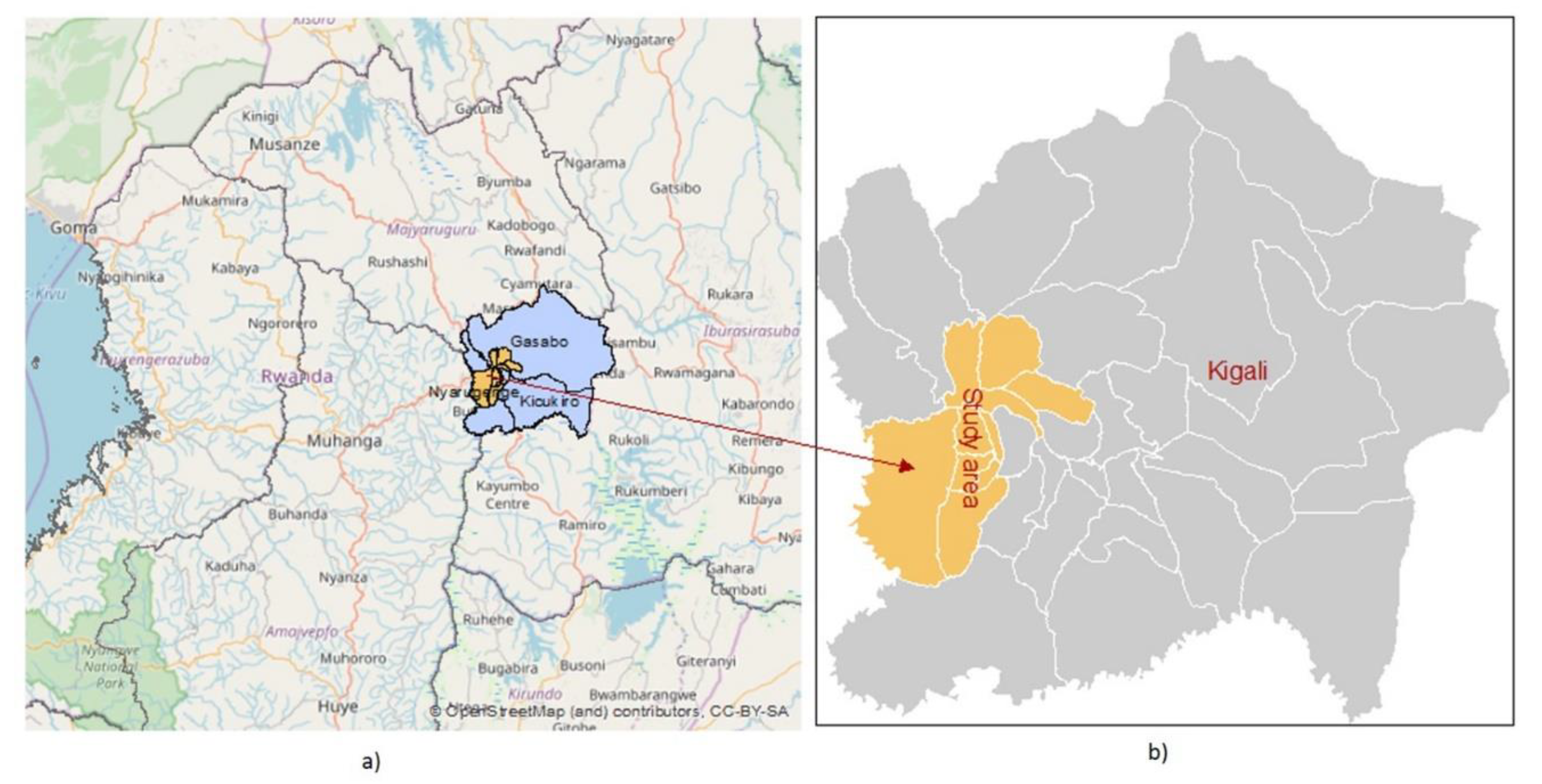
Figure 1. (a) Location of the city of Kigali in Rwanda (Source: OpenStreetMap base map), (b) the location of the study area in Kigali city.
Algorithms 13 00016 g001
Figure 2. An example of coding of a solution. The indices of the list represent the number of 10 building blocks while elements from 1 to 3 represent shelters. In this example, a population of 4 solutions is randomly generated.
Algorithms 13 00016 g002
Figure 3. An example of MSPSO particle mapped in continuous space and remapped in discrete space.
Algorithms 13 00016 g003
Figure 4. (a) Two-point crossover, and (b) mutation of an offspring.
Algorithms 13 00016 g004
Figure 5. Box plot of the average of the cost of four algorithms. (a) displays the full range of variation of the fitness values of capacity function, (b) displays the full range of variation of the fitness values of distance function. The outlier symbols (○, *) represent extreme values in data set of each method.
Algorithms 13 00016 g005
Figure 6. The final Pareto fronts of four algorithms with normalized fitness values. (a) Pareto front of AMOSA, (b) Pareto front of MOABC, (c) Pareto front of MSPSO, (d) Pareto front of NSGA-II.
Algorithms 13 00016 g006
Figure 7. Box plot of fitness variation and execution time of four algorithms. (a) displays the full range of variation of the fitness values of capacity function, (b) displays the full variation of the fitness values of distance function, and (c) variation mean of the execution time of 30 runs (in seconds). The outlier symbols (○, *) represent extreme values in data set of each method.
Algorithms 13 00016 g007
Figure 8. Convergence trends of the four algorithms. (a) AMOSA, (b) MOABC, (c) NSGA-II, (d) MSPSO.
Algorithms 13 00016 g008
Figure 9. Allocation maps of the shelters to building blocks from the case study area, when both capacity and distance objective functions are equally prioritized. (1) population allocation of AMOSA, (2) population allocation of MOABC, (3) population allocation of MSPSO, and (4) population allocation of NSGA-II.
Algorithms 13 00016 g009
Table 1. The parameter values of the four algorithms.
ParametersValue
AMOSA
Number of population100
Number of iterations500
Tmax100
Tmin10 × 10−3
Alpha (α)0.9
MOABC
Colony size100
Number of iterations500
Inertia Weight (w1)0.7
Inertia Weight (w2)0.8
MSPSO
Number of particles100
Number of iterations500
Acceleration constant (c1 = c2) 1.49
Inertia Weight (w)0.72
NSGA-II
Number of chromosomes100
Number of iterations500
cross-mutate rate 0.9
mutation rate0.01
Table 2. p-values of the Kruskal–Wallis test for evaluating the effectiveness and efficiency of four algorithms in both optimizing capacity and distance function.
KW TestEffectivenessEfficiency (Fitness Variation)Efficiency (Execution Time)
Cost of FcapacityCost of FdistanceCost of FcapacityCost of Fdistance
Chi-Square88.80998.016674.13162.42105.028
p-value0.0000.0000.0000.0000.000
Table 3. p-value of pairwise comparison of algorithms vs. t-statistic value of capacity and distance function.
IndexFcapacityFdistance
t-Statisticp-Valuet-Statisticp-Value
AMOSA-MOABC−3.2230.001 *−0.3930.852
AMOSA-MSPSO−17.1830.000 *−19.6930.000 *
MOABC-MSPSO−13.9600.000 *−19.3000.000 *
AMOSA-NSGA-II−9.0430.000 *−11.5490.000 *
MOABC-NSGA-II−5.8200.000 *−11.1560.000 *
MSPSO-NSGA-II8.1410.000 *8.1440.000 *
* p ≤ α.
Table 4. Comparison of fitness values of capacity and distance function (fcapacity & fdistance) for convergence speed.
IndexFcapacityFdistance
t-Statisticp-Valuet-Statisticp-Value
AMOSA-MOABC −11.2720.000 *−7.7100.000 *
AMOSA-MSPSO −23.0400.000 *−8.5540.000 *
MOABC-MSPSO −18.2210.000 *−1.3090.467
AMOSA-NSGA-II−3.0550.006 *−1.5750.340
MOABC-NSGA-II12.7160.000 *9.4950.000 *
MSPSO-NSGA-II30.9210.000 *10.7990.000 *
* p ≤ α.
Table 5. The variance of the best-normalized fitness values and average execution time of four algorithms. The minimum values are indicated in bold.
AlgorithmAverage Execution Time in Seconds The Variance of the Average-Normalized Fitness Values of Capacity Function The Variance of the Average-Normalized Fitness Values of the Distance Function
AMOSA736.670.0450.040
MOABC922.070.0500.052
MSPSO1786.900.0490.053
NSGA-II363.030.0560.081