Optimal Prefix Free Codes with Partial Sorting ^†

Abstract

We describe an algorithm computing an optimal prefix free code for n unsorted positive weights in time within $O\left(n\right(1+lg\alpha \left)\right)\subseteq O(nlgn)$, where the alternation $\alpha \in [1..n-1]$ approximates the minimal amount of sorting required by the computation. This asymptotical complexity is within a constant factor of the optimal in the algebraic decision tree computational model, in the worst case over all instances of size n and alternation $\alpha$. Such results refine the state of the art complexity of $\mathsf{\Theta }(nlgn)$ in the worst case over instances of size n in the same computational model, a landmark in compression and coding since 1952. Beside the new analysis technique, such improvement is obtained by combining a new algorithm, inspired by van Leeuwen’s algorithm to compute optimal prefix free codes from sorted weights (known since 1976), with a relatively minor extension of Karp et al.’s deferred data structure to partially sort a multiset accordingly to the queries performed on it (known since 1988). Preliminary experimental results on text compression by words show $\alpha$ to be polynomially smaller than n, which suggests improvements by at most a constant multiplicative factor in the running time for such applications.

1. Introduction

Given n positive weights $W[1..n]$ coding for the frequencies ${\left\{W\left[i\right]/{\sum }_{j=1}^{n}W\left[j\right]\right\}}_{i\in [1..n]}$ of n messages (We use the conveniently concise and general terminology of messages for the input and symbols for the output, as introduced by Huffman [1] himself, which should not be confused with other terminologies found in the literature, of input symbols, letters, or words for the input and output symbols or bits in the binary case for the output), and a constant number D of (output) symbols³, an optimal prefix free code [1] is a set of n code strings on the alphabet $[1..D]$, of variable lengths $L[1..n]$ such that no string is prefix of another, and the average length of a code is minimized (i.e., ${\sum }_{i=1}^{n}L\left[i\right]W\left[i\right]$ is minimal). The particularity of such codes is that even though the code strings assigned to the messages can differ in lengths (assigning shorter ones to more frequent messages yields compression to ${\sum }_{i=1}^{n}L\left[i\right]W\left[i\right]$ symbols), the prefix free property insures a non-ambiguous decoding.

Such optimal codes, known since 1952 [1], are used in “all the mainstream compression formats” [2] (e.g., PNG, JPEG, MP3, MPEG, GZIP, and PKZIP). “Huffman’s algorithm for computing minimum-redundancy prefix-free codes has almost legendary status in the computing disciplines” (Moffat [3]). The concept is “one of the fundamental ideas that people in computer science and data communications are using all the time” (Knuth [4]), and the code itself is “one of the enduring techniques of data compression. It was used in the venerable PACK compression program, authored by Szymanski in 1978, and remains no less popular today” (Moffat et al. [5] in 1997).

Even though some compression methods use only precomputed tables coding for an Optimal Binary Prefix Free Code “built-in” the compression method, there are still many applications that require the computation of such codes for each instance (e.g., BZIP2 [6], JPEG [7], etc.). In the current state of the art, the running time of such algorithm is almost never the bottleneck of the compression process, but nevertheless worth studying if only for theoretical sake, and potentially for future applications less directly related to compression: Takaoka [8,9,10] described an adaptive version of merge sort which scans for sorted runs in the input, and merge them according to a scheme which is exactly the Huffman code tree; and Barbay and Navarro [11] described how to use such code tree to compute the optimal shape of a wavelet tree for runs-based compression of permutations. This, in turns, has applications to the compression of general texts, via the compression of the permutations appearing in a Burrows Wheeler’s transform of the text.

1.1. Background

Any prefix free code can be computed in time linear in the input size from a set of code lengths satisfying the Kraft inequality ${\sum }_{i=1}^n{D}^{-L\left[i\right]}\le 1$. The original description of the code by Huffman [1] yields a heap-based algorithm performing $O(nlogn)$ algebraic operations, using the bijection between D-ary prefix free codes and D-ary cardinal trees [12]. In order to consider the optimality of this running time, one must notice that this algorithm is not in the comparison model (as it performs sums on elements of its input), but still in a quite restricted computational model, dubbed the algebraic decision tree computational model [13], composed of algorithms which can be modeled as a decision tree where decision nodes are based only on algebraic operations with a finite number of operators. In the algebraic decision tree computational model, the complexity of the algorithm suggested by Huffman [1] is asymptotically optimal for any constant value of D, in the worst case over instances composed of n positive weights, as computing the optimal prefix free code for the $(D\times n+1)$ weights $W[0,\dots ,Dn]=\{D^{x_1},\dots ,D^{x_1},D^{x_2},\dots ,D^{x_2},\dots ,D^{x_n},\dots ,D^{x_n}\}$ is equivalent to sorting the positive integers $\{x_1,\dots ,x_n\}$, a task proven to require $\mathsf{\Omega }(Dnlog(Dn\left)\right)=\mathsf{\Omega }(nlogn)$ (as D is a constant) in the algebraic decision tree model, by a simple argument of information theory.

Yet, not all instances require the same amount of work to compute an optimal code (see

Table 1. A selection of results on the computational complexity of optimal prefix free codes. n is the number of weights in the input; $r\in [1..n]$ is the number of distinct weights in the input; $k\in [1..n-1]$ is the number of distinct codelengths produced; and $\alpha \in [1..n-1]$ is the difficulty measure introduced in this work, the number of alternation between External nodes and Internal nodes in an execution of the algorithm suggested by Huffman [1] or by van Leeuwen’s algorithm [14] (see Section 3.1 for the formal definition).

Year	Name	Time	Space	Ref.	Note
1952	Huffman	$O(nlogn)$	$O\left(n\right)$	[1]	original
1976	van Leeuwen	$O\left(n\right)$	$O\left(n\right)$	[14]	sorted input
1995	Moffat and Katajainen	$O\left(n\right)$	$O\left(1\right)$	[18]	sorted input
1998	Moffat and Turpin	$O\left(r\right(1+log(n/r)\left)\right)$	“efficient”	[15]	compressed input and Output
2001	Milidiu et al.	$O\left(n\right)$	$O\left(1\right)$	[19]	sorted input
2006	Belal and Elmasry	$O\left({log}^{2k-1}n\right)$	$O\left(n\right)$	[16]	k distinct code lengths and sorted input
2006	Belal and Elmasry	potentially $O\left(kn\right)$	$O\left(n\right)$	[16]	k distinct code lengths
2005	Belal and Elmasry	$O\left({16}^{k}n\right)$	$O\left(n\right)$	[17]	k distinct code lengths
2016	Group-Dock-Mix	$O\left(n\right(1+log\alpha \left)\right)$	$O\left(n\right)$	[here]	$\alpha ={\left|\mathcal{S}\right|}_{EI}\in [1..n-1]$

for a partial list of relevant results):

• When the weights are given in sorted order, van Leeuwen [14] showed in 1976 that an optimal code can be computed using within $O\left(n\right)$ algebraic operations.
• When the weights consist of $r\in [1..n]$ distinct values and are given in a sorted, compressed form, Moffat and Turpin [15] showed in 1998 how to compute an optimal binary prefix free code using within $O\left(r\right(1+log(n/r)\left)\right)$ algebraic operations, which is sublinear in n when $r\in o\left(n\right)$.
• In the case where the weights are given unsorted, Belal and Elmasry [16,17] described in 2006 many families of instances for which an optimal binary prefix free code can be computed in linear time.

Such example of “easy instances” suggest that it could be possible to compute optimal prefix free codes in much less time by taking advantage of some measure of “easiness”, and indeed Belal and Elmasry [16,17] proposed an algorithm claimed to perform within $O\left(kn\right)$ algebraic operations, in the worst case over instances formed by n weights such that the binary prefix free code obtained by Huffman’s method [1] has exactly k distinct code lengths. The proof included in the proceedings yields only a bound within $O\left({16}^{k}n\right)$, while the claim of a complexity within $O\left(kn\right)$ was later downgraded to $O\left({16}^{k}n\right)$ in extended versions of their article published on public repositories [17]. Such result is asymptotically better than the state of the art when k is finite, but worse when k is larger than ${log}_{2}n$, which does not seem to be the case in practice (see our own experimental results in Table 3).

1.2. Question

In the context described above, we wondered about the existence of an algorithm taking advantage of small values of k, while behaving more reasonably than Belal and Elmasry’s solution [16,17] for large values of k (e.g., $k\in [logn\dots n-1]$). Kirkpatrick [20] defined a dovetailing combination of several algorithms as running all of them algorithms in parallel (not necessarily at the same rate) and stopping them all whenever one reaches the answer. We wonder if there is an algorithin more interestingly than a “dovetailing” combination of solutions running respectively in time within $O(nlogn)$ and $O\left(kn\right)$.

Given n positive integer weights, can one compute an optimal binary prefix free code in time within $o(min\{kn,nlogn\left\}\right)$ in the algebraic decision tree computational model for some general class of instances?

1.3. Contributions

We answer in the affirmative for many classes of instances (extending and formalizing the proofs of the same theoretical results previously described in 2016 [21]), identified by the “alternation” measure $\alpha \in [1..n-1]$ assigning a difficulty to each instance (formally defined in Section 3.1):

Theorem 1.

The computational complexity of optimal binary prefix free code is within $\mathsf{\Theta }\left(n\right(1+log\alpha \left)\right)$ in the algebraic decision tree computational model, in the worst case over instances of size n and alternation α.

Proof. 

We describe in Lemma 2 of Section 2.2 a deferred data structure which supports q queries of type rank, select and partialSum in time within $O\left(n\right(1+logq)+qlogn)$, all within the algebraic decision tree computational model. We describe in Section 2.3 the Group–Dock–Mix (GDM) algorithm, inspired by the van Leeuwen’s algorithm [14], modified to use this deferred data structure to compute optimal prefix free codes given an unsorted input, and we prove its correction in Lemma 3. We show in Lemma 8 that any algorithm A in the algebraic decision tree computational model performs within $\mathsf{\Omega }(nlog\alpha$) algebraic operations in the worst case over instances of size n and alternation $\alpha$. We show in Lemma 5 that the GDM algorithm performs $q\in O\left(\alpha (1+log\frac{n-1}{\alpha })\right)$ such queries, which yields in Corollary 6 a complexity within $O(n(1+log\alpha )+\alpha (logn)(log\frac{n}{\alpha }))$, all within the algebraic decision tree computational model. As $\alpha \in [1..n-1]$ and $O\left(\alpha (logn)(log\frac{n}{\alpha })\right)\subseteq O\left(n(1+log\alpha )\right)$ for this range (Lemma 7), the asymptotic optimality ensues. □

When $\alpha$ is at its maximal (i.e., $\alpha =n-1$), this complexity matches the tight asymptotic computational complexity bound of $\mathsf{\Theta }(nlogn)$ for algorithms in the algebraic decision tree computational model in the worst case over all instances of size n. When $\alpha$ is substantially smaller than n (e.g., $\alpha \in O(logn)$, which practicality we discuss in Section 4), the GDM algorithm performs within $o(nlogn)$ operations, down to linear in n for finite values of $\alpha$.

Another natural question is whether practical instances present small enough values of parameters such as k and $\alpha$ that taking advantage of them makes a difference. By a preliminary set of experiments on word-based compression of English texts, we answer with a tentative negation (this experimentation is a new addition to the previous presentation of this work [21]). The alternation $\alpha$ of practical instances is much smaller than the number n of weights, with ratios (see Table 3 for more similar values) from 77 ($\alpha =40$ and $n=3099$) to 154 ($\alpha =440$ and $n=$ 67,780). However, it does not seem to be small enough to make a meaningful difference in term of running time, as $log\alpha \ge \frac{1}{2}logn$ on the data set, which suggests that such instances are not “easy enough” for such techniques to make a meaningful difference in running time. We obtain similar results about the parameter k, with $k>logn$ for all instances of the data set, rendering a solution running in time within $O\left(kn\right)$ non competitive compared either to the state of the art solution running in time within $O(nlogn)$, nor to the solution proposed in this work running in time within $O\left(n\right(1+log\alpha \left)\right)$.

In the next section (Section 2), we describe our solution in three parts: the intuition behind the general strategy in Section 2.1, the deferred data structure which maintains a partially sorted list of weights while supporting rank, select and partialSum queries in Section 2.2, and the algorithm which uses those operators to compute an optimal prefix free code in Section 2.3. Our most technical contribution consists in the analysis of the running time of this solution, described in Section 3: the formal definition of the parameter of the analysis in Section 3.1, the upper bound in Section 3.2 and the matching lower bound in Section 3.3. In Section 4, we compare the experimental values of the difficulty measures over unordered instances of the optimal prefix free code computation on a sample of texts, the alternation $\alpha$ introduced in this work and the number k of distinct code lengths proposed by Belal and Elmasry [16,17]. We conclude with a theoretical comparison of our results with those from Belal and Elmasry [16,17] in Section 5, along with a discussion of potential themes for further research.

2. Solution

The solution that we describe is a combination of two results: some results about deferred data structures for multisets, which support queries in a “lazy” way; and some results about optimal prefix free codes themselves, about the relation between the computational cost of partially sorting a set of positive integers and the computational cost of computing a binary optimal prefix free code for the corresponding frequency distribution. We describe the general intuition of our solution in Section 2.1, the deferred data structure in Section 2.2, and the algorithm in Section 2.3.

2.1. General Intuition

Observing that the algorithm suggested by Huffman [1] in 1952 always creates the internal nodes in increasing order of weight, van Leeuwen [14] described in 1976 an algorithm to compute optimal prefix free codes in linear time when the input (i.e., the weights of the external nodes) is given in sorted order. A close look at the execution of van Leeuwen’s algorithm [14] reveals a sequence of sequential searches for the insertion rank r of the weight of some internal node in the list of weights of external nodes. Such sequential search could be replaced by a more efficient search algorithm in order to reduce the number of comparisons performed (e.g., a doubling search [22] would find such a rank r in $2\lceil {log}_{2}r\rceil$ comparisons instead of the r comparisons spent by a sequential search). Of course, this would reduce the number of comparisons performed, but it would not reduce the number of algebraic operations (in this case, sums) performed, and hence neither would it significantly reduce the total running time of the algorithm.

Example 1.

Consider the following instance for the computation of a optimal prefix free code formed by $n=16$ sorted positive weights $W=$ such that the first internal node created has larger weight than the largest weight in the original array (i.e., $W\left[1\right]+W\left[2\right]=16+17=33>W\left[16\right]=31$). On such an instance, van Leeuwen’s algorithm [14] starts by performing $n-2=14$ comparisons in the equivalent of a sequential search in W for $W\left[1\right]+W\left[2\right]=33$: a binary search would perform $\lceil {log}_{2}n\rceil =4$ comparisons instead, and a doubling search [22] no more than $2\lceil {log}_{2}n\rceil =8$ comparisons.

As mentioned above, any algorithm must access (and sum) each weight at least once in order to compute an optimal prefix free code for the input, so that reducing the number of comparisons does not reduce the running time of van Leeuwen’s algorithm on a sorted input, but it illustrates how instances with clustered external and internal nodes are “easier” than instances in which they are interleaved.

The algorithm suggested by Huffman [1] starts with a heap of external nodes, selects the two nodes of minimal weight, pair them into a new node which it adds to the heap, and iterates till only one node is left. Whereas the type of the nodes selected, external or internal, does not matter in the analysis of the complexity of Huffman’s algorithm, we claim that the computational cost of optimal prefix free codes can be greatly reduced on instances where many external nodes are selected consecutively. We define the “EI signature” of an instance as the first step toward the characterization of such instances:

Definition 1 (EI signature).

Given an instance of the optimal prefix free code problem formed by n positive weights $W[1..n]$, its EI signature $\mathcal{S}\left(W\right)\in {\{E,I\}}^{2n-1}$ is a string of length $2n-1$ over the alphabet $\{E,I\}$ (where E stands for “external” and I for “internal”) marking, at each step of the algorithm suggested by Huffman [1], whether an external or internal node is chosen as the minimum (including the last node returned by the algorithm, for simplicity).

The analysis described in Section 3 is based on the number ${\left|\mathcal{S}\right|}_{EI}$ of maximal blocks of consecutive positions formed only of E in the EI signature of the instance $\mathcal{S}$. We can already show some basic properties of this measure:

Lemma 1.

Given the EI signature $\mathcal{S}$ of n unsorted positive weights $W[1..n]$,

1. 

The number of occurrences ${\left|\mathcal{S}\right|}_E$ of E in the signature $\mathcal{S}$ is ${\left|\mathcal{S}\right|}_E=n$;

2. 

The number of occurrences ${\left|\mathcal{S}\right|}_I$ of I in the signature $\mathcal{S}$ is ${\left|\mathcal{S}\right|}_I=n-1$;

3. 

The length $\left|\mathcal{S}\right|$ of the signature $\mathcal{S}$ is their sum, $\left|\mathcal{S}\right|=2n-1$;

4. 

The signature $\mathcal{S}$ starts with two E;

5. 

The signature $\mathcal{S}$ finishes with one I;

6. 

The number ${\left|\mathcal{S}\right|}_{EI}$ of consecutive occurrences of $EI$ in the signature $\mathcal{S}$ is one more than the number of occurrences of $IE$ in it, ${\left|\mathcal{S}\right|}_{EI}={\left|\mathcal{S}\right|}_{IE}+1$;

7. 

The number ${\left|\mathcal{S}\right|}_{EI}$ of consecutive occurrences of $EI$ in the signature $\mathcal{S}$ is at least 1 and at most $n-1$, ${\left|\mathcal{S}\right|}_{EI}\in [1..n-1]$.

Proof. 

The three first properties are simple consequences of basic properties on binary trees. $\mathcal{S}$ starts with two E as the first two nodes paired are always external. $\mathcal{S}$ finishes with one I as the last node returned is always (for $n>1$) an internal node. The two last properties are simple consequences of the fact that $\mathcal{S}$ is a binary string starting with an E and finishing with an I. □

Example 2.

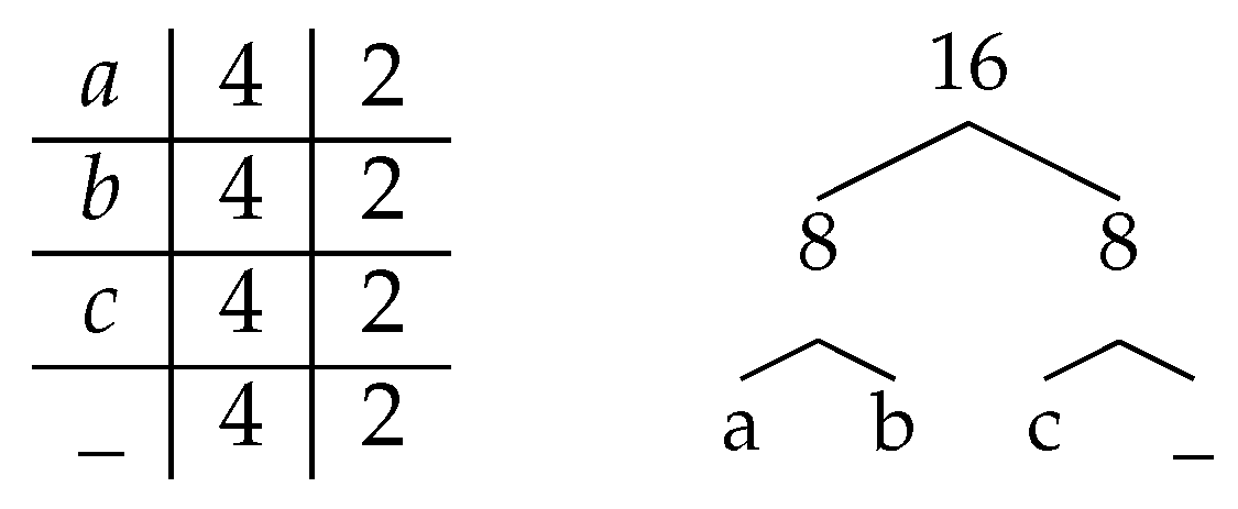
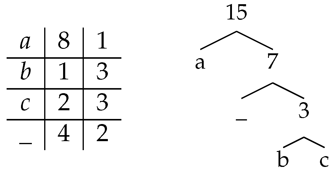
For example, consider the text $T=$ “ABBCCCDDDDEEEEEFFFFFGGGGGGHHHHHHH” formed by the concatenation of one occurrence of “A”, two occurrences of “B”, three occurrences of “C”, four occurrences of “D”, five occurrences of “E”, five (again) occurrences of “F”, six occurrences of “G” and seven occurrences of “H”, so that the corresponding frequencies are $W=$ . It corresponds to an instance of size $n=8$, of EI signature $\mathcal{S}\left(W\right)=\mathbf{EE}\underline{\mathbf{E}}\underline{\mathtt{I}}\mathbf{EEE}\underline{\mathbf{E}}\underline{\mathtt{I}}\underline{\mathbf{E}}\underline{\mathtt{I}}\mathtt{IIII}$ of length 15, which starts with $\mathbf{EE}$, finishes with I, and contains only $\alpha =3$ occurrences of $\underline{\mathbf{E}I}$ (underlined), corresponding to a decomposition into $\alpha =3$ maximal blocks of consecutive $\mathbf{E}$s (in bold), out of a maximal potential number of 7 for the alphabet size $n=8$.

Instances such as that presented in Example 2, with very few blocks of E (more than in Example 3, but much less than in the worst case), are easier to solve than instances with many such blocks. For example, an instance W of length n such that its EI signature $\mathcal{S}\left(W\right)$ is composed of a single run of nEs followed by a single run of $n-1$Is (such as the one described in Figure 1) can be solved in linear time, and in particular without sorting the weights: it is enough to assign the codelength $l=\lfloor {log}_{2}n\rfloor$ to the $n-2^l$ largest weights and the codelength $l+1$ to the $2^l$ smallest weights. Separating those weights is a simple select operation, supported in amortized linear time by the data structures described in the following section. We describe two other extreme examples, starting with one where all the weights are equal (as a particular case of when they are all within a factor of two of each other).

Example 3.

Consider the text $T=$ “ba_bb_caca_ba_cc” from Figure 1. Each of the four messages (input symbols) of its alphabet $\{a,b,c,\_\}$ occurs exactly 4 times, so that an optimal prefix free code assigns a uniform codelength of 2 bits to all messages (see Figure 1). There is no need to sort the messages by frequency (and the prefix free code does not yield any information about the order in which the messages would be sorted by monotone frequencies), and accordingly the EI signature of this text, $\mathcal{S}\left(T\right)=$ “EEE EI II”, has a single block of Es, indicating a very easy instance. The same holds if the text is such that the frequencies of the messages are all within a factor of two of each other.

On the other hand, some instances present the opposite extreme, where no weight is within a factor of two of any other, which “forces” any algorithm computing optimal prefix free codes to sort the weights.

Example 4.

Consider the text $T=$ “aaaaaaaabcc____” from Figure 2 (composed of one occurrence of “b”, two occurrences of “c”, four occurrences of “_”, and eight occurrences of “a”), such that the frequencies of its messages follow an exponential distribution, so that an optimal prefix free code assigns different codelengths to almost all messages (see the third column of the array in Figure 2). Any optimal prefix free code for this instance yields all the information required to sort the messages by frequencies. Accordingly, the EI signature $\mathcal{S}\left(T\right)=$ “E EIEIEI” of this instance has three blocks of Es (out of three possible ones) for this value of the alphabet size $n=4$, indicating a more difficult instance. The same holds with more general distributions, as long as no two pairs of message frequencies are within a factor of two of each other.

Those various examples should give an intuition of the features of the instance that our techniques aim to take advantage of. We describe those techniques more formally in the two following sections, starting with the deferred data structure allowing to partially sort the weights in Section 2.2, and following with the algorithm itself in Section 2.3.

2.2. Partial Sum Deferred Data Structure

Given a multiset $W[1..n]$ of size n on an alphabet $[1..\sigma ]$ of size $\sigma$, Karp et al. [23] defined the first deferred data structure supporting for all $x\in [1..\sigma ]$ and $r\in [1..n]$ queries such as rank$\left(x\right)$, the number of elements which are strictly smaller than x in W; and select$\left(r\right)$, the value of the r-th smallest value (counted with multiplicity) in W. Their data structure supports q queries in time within $O\left(n\right(1+logq)+qlogn)$, all in the comparison model (Karp et al.’s result [23] is actually better than this formula when the number of queries q is larger than the size n of the multiset, but such configuration does not occur in the case of the computation of an optimal prefix free code, where the number q of queries is always smaller or equal to n: for simplicity, we summarize their result as $O\left(n\right(1+logq)+qlogn)$). To achieve this results, it partially sorts its data in order to minimize the computational cost of future queries, but avoids sorting all of the data if the set of queries does not require it: the queries have then become operators in some sense (they modify the data representation). Note that whereas the running time of each individual query depends on the state of the data representation, the answer to each query is itself independent of the state of the data representation.

Karp et al.’s data structure [23] supports only rank and select queries in the comparison model, whereas the computation of optimal prefix free codes requires to sum pairs of weights from the input, and the algorithm that we propose in Section 2.3 requires to sum weights from a range in the input. Such requirement can be reduced to partialSum queries. Whereas partialSum queries have been defined in the literature based on the positions in the input array, we define such queries here in a way that depends only on the content of the multiset (as opposed to a definition depending on the order in which the multiset is given in the input), so that it can be generalized to deferred data structures.

Definition 2 (Partial sum data structure).

Given n unsorted positive weights $W[1..n]$, a partial sum data structure supports the following queries:

• rank$\left(x\right)$, the number of elements which are strictly smaller than x in W;
• select$\left(r\right)$, the value of the r-th smallest value (counted with multiplicity) in W;
• partialSum$\left(r\right)$, the sum of the r smallest elements (counted with multiplicity) in W.

Example 5.

Given the array $A=$ ,

• the number of elements strictly smaller than 5 is rank$\left(5\right)=4$,
• the sixth smallest value is select$\left(6\right)=5$ (counting with redundancies), and
• the sum of the two smallest elements is partialSum$\left(2\right)=3$.

We describe below how to extend Karp et al.’s deferred data structure [23], which already supports rank and select queries on multisets, in order to add the support for partialSum queries, with an amortized running time within a constant factor of the asymptotic time of the original solution. Note that the operations performed by the data structure are not any more within the comparison model, but rather in the algebraic decision tree computational model, as they introduce algebraic operations (additions) on the elements of the multiset. The result is a direct extension of Karp et al. [23], adding a sub-task taking linear time (updating partial sums in an interval of positions) to a sub-task which was already taken linear time (partitioning this same interval by a pivot):

Lemma 2.

Given n unsorted positive weights $W[1..n]$, there is a partial sum deferred data structure which supports q operations of type rank, select, and partialSum in time within $O\left(n\right(1+logq)+qlogn)$, all within the algebraic decision tree computational model.

Proof. 

Karp et al. [23] described a deferred data structure which supports the rank and select queries (but not partialSum queries). It is based on median computations and $(2,3)$-trees, and performs q queries on n values in time within $O\left(n\right(1+logq)+qlogn)$, all within the comparison model (and hence in the even less restricted algebraic decision tree computational model). We describe below how to modify their data structure in a simple way, so that to support partialSum queries with asymptotically negligible additional cost.

At the initialization of the data structure, compute the n partial sums corresponding to the n positions of the unsorted array. After each median computation and partitioning in a rank or select query, recompute the partial sums on the range of values newly partitioned, which increases the cost of the query only by a constant factor. When answering a partialSum query, perform a select query, and then return the value of the partial sum corresponding to the value by the select query: the asymptotic complexity is within a constant factor of the one described by Karp et al. [23]. □

Barbay et al. [24] further improved Karp et al.’s result [23] with a simpler data structure (a single binary array) and a finer analysis taking into account the gaps between the positions hit by the queries. Barbay et al.’s results [24] can similarly be augmented in order to support partialSum queries while increasing the computational complexity by only a constant factor. This finer result is not relevant to the analysis described in Section 3, given the lack of specific features of the distribution of the gaps between the positions hits by the queries, as generated by the GDM algorithm described in Section 2.3.

Such a deferred data structure is sufficient to simply execute van Leeuwen’s algorithm [14] on an unsorted array of positive integers, but would not result in an improvement in the computational complexity: such a simple variant of van Leeuwen’s algorithm [14] is simply performing n select operations on the input, effectively sorting the unsorted array. We describe in the next section an algorithm which uses the deferred data structure described above to batch the operations on the external nodes, and to defer the computation of the weights of some internal nodes to later, so that for many instances the input is not completely sorted at the end of the execution, which indeed reduces the total cost of the execution of the algorithm.

2.3. Algorithm “Group–Dock–Mix” (GDM) for the Binary Case

There are five main phases in the GDM algorithm: the initialization, three phases (grouping, docking, and mixing, giving the name “GDM” to the algorithm) inside a loop running until only internal nodes are left to process, and the conclusion:

• In the initialization phase, initialize the partial sum deferred data structure with the input, and the first internal node by pairing the two smallest weights of the input.
• In the grouping phase, detect and group the weights smaller than the smallest internal node: this corresponds to a run of consecutive E in the EI signature of the instance.
• In the docking phase, pair the consecutive positions of those weights (as opposed to the weights themselves, which can be reordered by future operations) into internal nodes, and pair those internal nodes until the weight of at least one such internal node becomes equal or larger than the smallest remaining weight: this corresponds to a run of consecutive I in the EI signature of the instance.
• In the mixing phase, rank the smallest unpaired weight among the weights of the available internal nodes, and pairs the internal node of smaller weight two by two, leaving the largest one unpaired: this corresponds to an occurrence of $IE$ in the EI signature of the instance. This is the most complicated (and most costly) phase of the algorithm.
• In the conclusion phase, with i internal nodes left to process (and no external node left), assign codelength $l=\lfloor {log}_{2}i\rfloor$ to the $i-2^l$ largest ones and codelength $l+1$ to the $2^l$ smallest ones: this corresponds to the last run of consecutive I in the EI signature of the instance.

The algorithm and its complexity analysis distinguish two types of internal nodes: pure nodes, which descendants were all paired during the same grouping phase; and mixed nodes, each of which either is the ancestor of such a mixed node, or pairs a pure internal node with an external node, or pairs two pure internal nodes produced at distinct phases of the GDM algorithm. The distinction is important as the algorithm computes the weight of any mixed node at its creation (potentially generating several data structure operations), whereas it defers the computation of the weight of some pure nodes to later, and does not compute the weight of some pure nodes. We will discuss this further in Section 5 about the non istance optimality of the solution presented.

Before describing each phase more in detail, it is important to observe the following invariant of the algorithm:

Property 1.

Given an instance of the optimal binary prefix free code problem formed by $n>1$ positive weights $W[1..n]$, between each phase of the algorithm, all unpaired internal nodes have weight within a constant factor of two (i.e., the maximal weight of an unpaired internal node is strictly smaller than twice the minimal weight of an unpaired internal node).

Proof. 

The generally property is proven by checking that each phase preserves it:

• Initialization: there is only one internal node at the end of this phase, hence the conditions for the property to stand are created.
• Grouping: no internal node is created, hence the property is preserved.
• Docking: pairing until at least one internal node has weight equal or larger than the smallest weight of a remaining weight (future external node) insures the property.
• Mixing: as this phase pairs all internal nodes except possibly the one of largest weight, the property is preserved.
• Conclusion: A single node is left at the end of the phase, hence the property.

As the initialization phase creates the property and each other phase preserves it, the property is verified through the execution of the algorithm. □

We now proceed to describe each phase in more details:

• Initialization: Initialize the deferred data structure partial sum with the input; compute the weight currentMinInternal of the first internal node through the operation partialSum$\left(2\right)$ (the sum of the two smallest weights); create this internal node, of weight currentMinInternal and children 1 and 2 (the positions of the first and second weights, in any order); compute the weight currentMinExternal of the first unpaired weight (i.e., the first available external node) by the operation select$\left(3\right)$; setup the variables nbInternals $=1$ and nbExternalProcessed $=2$.
• Grouping: Compute the position r of the first unpaired weight larger than the smallest unpaired internal node, through the operation rank(currentMinInternal); pair the (($r-\mathrm{nbExternalProcessed}$) modulo 2) indices to form $\lfloor \frac{r-\mathrm{nbExternalProcessed}}{2}\rfloor$ pure internal nodes; compute the parity of the number $r-\mathrm{nbExternalProcessed}$ of unpaired weights smaller than the first unpaired internal node; if it is odd, select the r-th weight through the operation $\mathrm{select}\left(r\right)$, compute the weight of the first unpaired internal node, compare it with the next unpaired weight, to form one mixed node by combining the minimal of the two with the extraneous weight.
• Docking: Pair all internal nodes by batches (by Property 1, their weights are all within a factor of two, so all internal nodes of a generation are processed before any internal node of the next generation); after each batch, compare the weight of the largest such internal node (compute it through $\mathrm{partialSum}$ on its range if it is a pure node, otherwise it is already computed) with the first unpaired weight: if smaller, pair another batch, and if larger, the phase is finished.
• Mixing: Rank the smallest unpaired weight among the weights of the available internal nodes, by a doubling search starting from the beginning of the list of internal nodes. For each comparison, if the internal node’s weight is not already known, compute it through a partialSum operation on the corresponding range (if it is a mixed node, it is already known). If the number r of internal nodes of weight smaller than the unpaired weight is odd, pair all but one, compute the weight of the last one and pair it with the unpaired weight. If r is even, pair all of the r internal nodes of weight smaller than the unpaired weight, compare the weight of the next unpaired internal node with the weight of the next unpaired external node, and pair the minimum of the two with the first unpaired weight. If there are some unpaired weights left, go back to the Grouping phase, otherwise continue to the Conclusion phase.
• Conclusion: There are only internal nodes left, and their weights are all within a factor of two from each other. Pair the nodes two by two in batch as in the docking phase, computing the weight of an internal node only when the number of internal nodes of a batch is odd.

The combination of those phases forms the GDM algorithm, which computes an optimal prefix free code given an unsorted sets of positive integers.

Lemma 3.

The tree returned by the GDM algorithm describes an optimal binary prefix free code for its input.

In the next section, we analyze the number q of rank, select and partialSum queries performed by the GDM algorithm, and deduce from it the complexity of the algorithm in term of algebraic operations.

3. Analysis

The GDM algorithm runs in time within $O(nlogn)$ in the worst case over instances of size n (which is optimal (if not a new result) in the algebraic decision tree computational model). However, it runs much faster on instances with few blocks of consecutive Es in the EI signature of the instance. We formalize this concept by defining the alternation $\alpha$ of the instance in Section 3.1. We then proceed in Section 3.2 to show upper bounds on the number of queries to the deferred data structure and algebraic operations on the data performed by the GDM algorithm in the worst case over instances of fixed size n and alternation $\alpha$. We finish in Section 3.3 with a matching lower bound for the number of operations performed by any algorithm in the algebraical decision tree model.

3.1. Parameter Alternation $\alpha \left(W\right)$

We suggested in Section 2.1 that the number ${\left|\mathcal{S}\right|}_{EI}$ of blocks of consecutive Es in the EI signature of an instance can be used to measure its difficulty. Indeed, some “easy” instances have few such blocks, and the instance used to prove the $\mathsf{\Omega }(nlogn)$ lower bound on the computational complexity of optimal prefix free codes in the algebraic decision tree computational model in the worst case over instances of size n has $n-1$ such blocks (the maximum possible in an instance of size n). We formally define this measure as the “alternation” of the instance (it measures how many times the algorithm suggested by Huffman [1] or the van Leeuwen algorithm [14] “alternates” from an external node to an internal node in its iterative selection process for nodes of minimum weight) and denote it by the parameter $\alpha$:

Definition 3 (Alternation).

Given an instance of the optimal binary prefix free code problem formed by n positive weights $W[1..n]$, its alternation $\alpha \left(W\right)\in [1..n-1]$ is the number of occurrences of the substring “$EI$” in its EI signature $\mathcal{S}\left(W\right)$.

In other words, the alternation $\alpha \left(W\right)\in [1..n-1]$ of W is the number of times that the algorithm suggested by Huffman [1] or the van Leeuwen’s algorithm [14] selects an internal node immediately after selecting an internal node.

Note that counting the number of blocks of consecutive Es is equivalent to counting the number of blocks of consecutive Is: they are the same, because the EI signature starts with two Es and finishes with an I, and each new I-block ends an E-block and vice-versa. Also, the choice between measuring the number of occurrences of “$EI$” or the number of occurrence of “$IE$” is arbitrary, as they are within a term of 1 of each other (see Section 3.1): counting the number of occurrences of “$EI$” just gives a nicer range of $[1..n-1]$ (as opposed to $[0..n-2]$). This number is of particular interest as it measures the number of iteration of the main loop in the GDM algorithm:

Lemma 4.

Given an instance of the optimal prefix free code problem of alternation α, the GDM algorithm performs α iterations of its main loop.

Proof. 

This is a direct consequence of the definition of the alternation $\alpha$ on one hand, and of the definition of the algorithm GDM on the other hand.

The main loop consists in three phases, respectively named grouping, docking, and mixing. The grouping phase corresponds to the detection and grouping of the weights smaller than the smallest internal node: this corresponds to a run of consecutive E in the EI signature of the instance. The docking phase corresponds to the pairing of the consecutive positions of those weights into internal nodes, and of those internal nodes though produced, recusively until the weight of at least one such internal node becomes equal or larger than the smallest remaining weight: this corresponds to a run of consecutive I in the EI signature of the instance. The mixing phase corresponds to the ranking of the smallest unpaired weight among the weights of the available internal nodes: this corresponds to an occurrence of $IE$ in the EI signature of the instance.

As the iterations of the main loop of the GDM algorith are in bijection with the runs of consecutive E in the EI signature of the instance, the number of such iteration is the number $\alpha$ of such runs. □

In the next section, we refine this result to the number of data structure operations and algebraic operations performed by the GDM algorithm.

3.2. Running Time Upper Bound

In order to measure the number of queries performed by the GDM algorithm, we detail how many queries are performed in each phase of the algorithm.

• The initialization corresponds to a constant number of data structure operations: a select operation to find the third smallest weight (and separate it from the two smallest ones), and a simple partialSum operation to sum the two smallest weights of the input.
• Each grouping phase corresponds to a constant number of data structure operations: a partialSum operation to compute the weight of the smallest internal node if needed, and a rank operation to identify the unpaired weights which are smaller or equal to that of this node.
• The number of operations performed by each docking and mixing phase is better analyzed together: if there are i “I” in the I-block corresponding to this phase in the EI signature, and if the internal nodes are grouped on h levels before generating an internal node of weight larger than the smallest unpaired weight, the docking phase corresponds to at most h partialSum operations, whereas the mixing phase corresponds to at most ${log}_2(i/2^h)$ partialSum operations, which develops to ${log}_2\left(i\right)-h$, for a total of $h+{log}_2\left(i\right)-h={log}_{2}i$ data structure operations.
• The conclusion phase corresponds to a number of data structure operations logarithmic in the size of the last block of Is in the EI signature of the instance: in the worst case, the weight of one pure internal node is computed for each batch, through one single partialSum operation each time.

Lemma 4 and the concavity of the logarithm function yields the total number of data structure operations performed by the GDM algorithm:

Lemma 5.

Given an instance of the optimal binary prefix free code problem of alternation α, the GDM algorithm performs within $O\left(\alpha (1+log\frac{n-1}{\alpha })\right)$ data structure operations on the deferred data structure given as input.

Proof. 

For $i\in [1..\alpha ]$, let $n_i$ be the number of internal nodes at the beginning of the i-th docking phase. According to Lemma 4 and the analysis of the number of data structure operations performed in each phase, the GDM algorithm performs in total within $O(\alpha +{\sum }_{i=1}^{\alpha }log{n}_i)$ data structure operations. Since there are at most $n-1$ internal nodes and the sum ${\sum }_{i=1}^{\alpha }{n}_i\le n-1$, by concavity of the logarithm the number of queries is within $O(\alpha +\alpha log\frac{n-1}{\alpha })=O\left(\alpha (1+log\frac{n-1}{\alpha })\right)$. □

Combining this result with the complexity of the partialSum deferred data structure from Lemma 2 directly yields the complexity of the GDM algorithm in algebraic operation (and running time):

Lemma 6.

Given an instance of the optimal binary prefix free code problem of alternation α, the GDM algorithm runs in time within $O(n(1+log\alpha )+\alpha (logn)(1+log\frac{n-1}{\alpha }))$, all within the algebraic decision tree computational model.

Proof. 

Let q be the number of queries performed by the GDM algorithm. Lemma 5 implies that $q\in O\left(\alpha (1+log\frac{n-1}{\alpha })\right)$. Plunging this into the expression $O\left(n\right(1+logq)+qlogn)$ from Lemma 2 yields a complexity within $O(n(1+log\alpha )+\alpha (logn)(1+log\frac{n-1}{\alpha }))$. □

Some simple functional analysis further simplifies the expression to our final upper bound:

Lemma 7.

Given two positive integers $n>0$ and $\alpha \in [1..n-1]$,

$$O\left(\alpha (logn)(log\frac{n}{\alpha })\right)\subseteq O\left(n(1+log\alpha )\right)$$

Proof. 

Given two positive integers $n>0$ and $\alpha \in [1..n-1]$, $\alpha <\frac{n}{logn}$ and $\frac{\alpha }{log\alpha }<n$. A simple rewriting yields $\frac{\alpha }{log\alpha }<\frac{n}{{log}^{2}n}$ and $\alpha {log}^{2}n>nlog\alpha$. Then, $n/\alpha <n$ implies $\alpha \times logn\times log\frac{n}{\alpha }<nlog\alpha$, which yields the result. □

In the next section, we show that this complexity is indeed optimal in the algebraic decision tree computational model, in the worst case over instances of fixed size n and alternation $\alpha$.

3.3. Lower Bound

A complexity within $O\left(n\right(1+log\alpha \left)\right)$ is exactly what one could expect, by analogy with multiset sorting: there are $\alpha$ groups of weights, so that the order within each groups does not matter much, but the order between weights from different groups does matter. We combine two results:

• a linear time reduction from multiset sorting to the computation of optimal prefix free codes; and
• the lower bound within $\mathsf{\Omega }(nlog\alpha )$ (tight in the comparison model) suggested by information theory for the computational complexity of multiset sorting in the worst case over multisets of size n with at most $\alpha$ distinct elements.

This yields a lower bound within $\mathsf{\Omega }(nlog\alpha )$ on the computational complexity of computing optimal binary prefix free codes in the worst case over instances of size n and alternation $\alpha$.

Lemma 8.

Given the integers $n\le 2$ and $\alpha \in [1..n-1]$, for any correct algorithm A computing optimal binary prefix free codes in the algebraic decision tree computational model, there is a set $W[1..n]$ of n positive weights of alternation α such that A performs within $\mathsf{\Omega }(nlog\alpha$) algebraic operations.

Proof. 

For any Multiset $A[1..n]=\{x_1,\dots ,x_n\}$ of n values from an alphabet of $\alpha$ distinct values, define the instance $W_A=\{2^{x_1},\dots ,2^{x_n}\}$ of size n, so that computing an optimal prefix free code for W, sorted by code length, provides an ordering for A. W has alternation $\alpha$: for any two distinct values x and y from A, the algorithm suggested by Huffman [1] as well as van Leeuwen’s algorithm [14] pair all the weights of value $2^x$ before pairing any weight of value $2^y$, so that the EI signature of $W_A$ has $\alpha$ blocks of consecutive Es. The lower bound then results from the classical lower bound on sorting mmultisets in the comparison model in the worst case over multisets of size n with $\alpha$ distinct values [25], itself based on the number ${\alpha }^n$ of possible such multisets. □

Having shown that the GDM algorithm takes optimally advantage of $\alpha$, we are left to check whether values of $\alpha$ in practice are small enough for GDM’s improvements to be worth of notice. We show in the next section that, at least for one application, it does not seem to be the case.

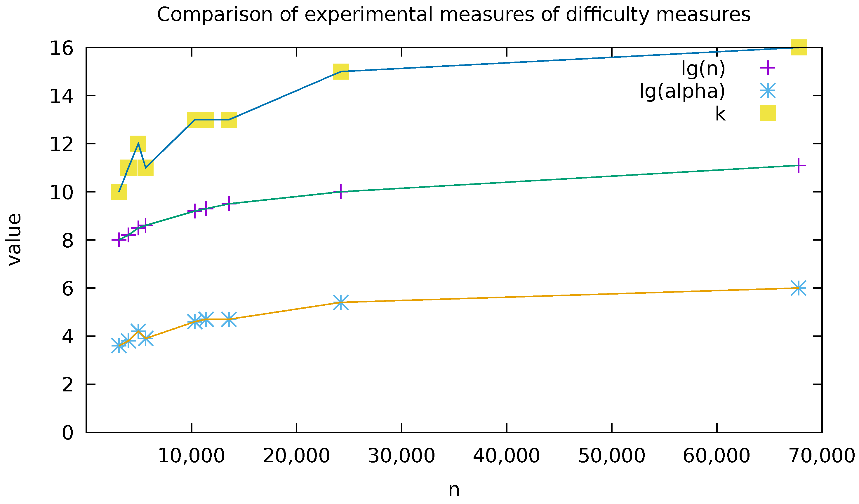
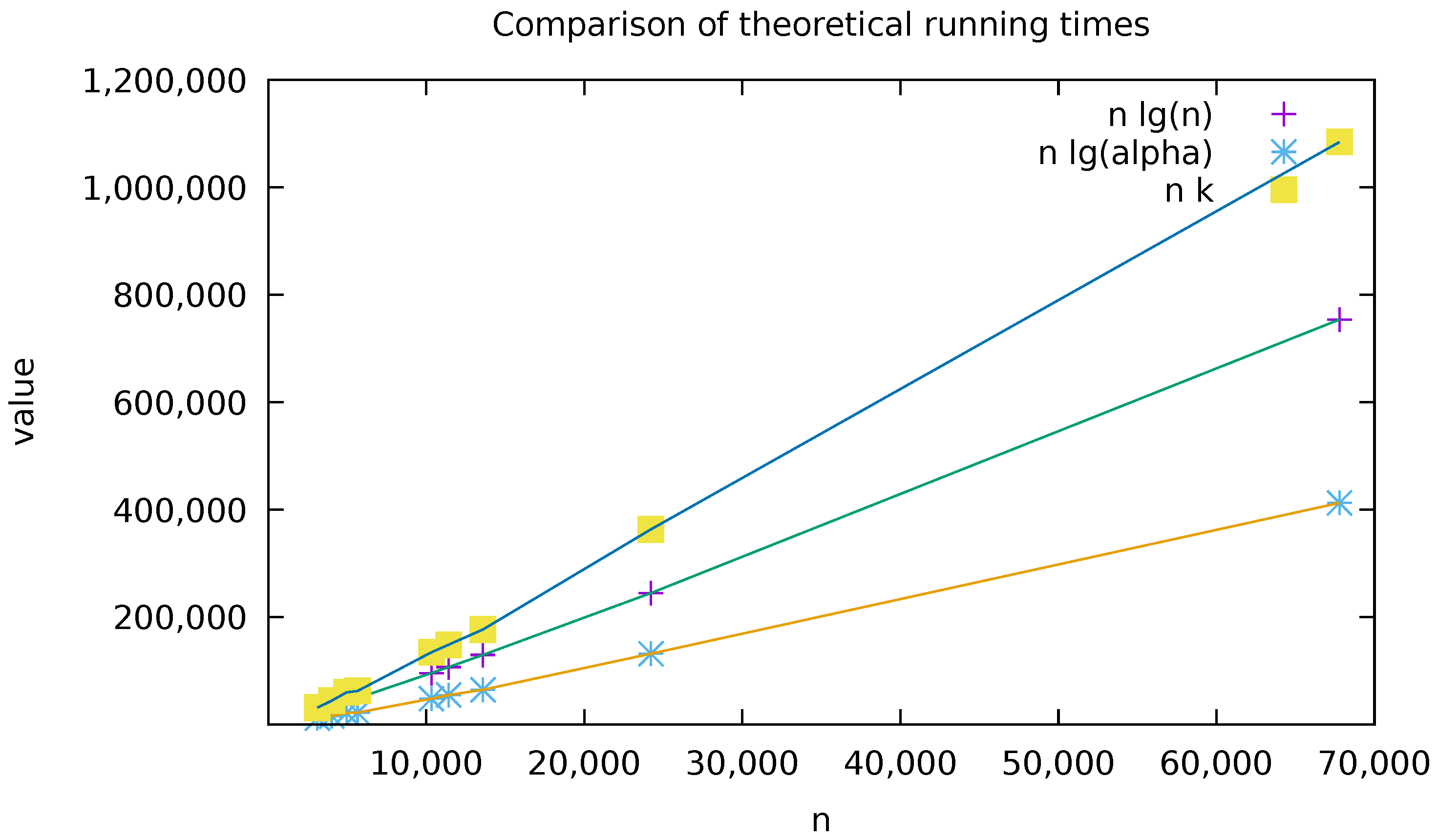
4. Preliminary Experimentations

There are many mature implementations [5,18] to compute optimal prefix free codes: Huffman’s solution [1] to the problem of optimal prefix free codes is not only ancient (67 years from 1952 to 2019), but also one still in wide use: In 1991, Gary Stix stated that “products that use Huffman code might fill a consumer electronics store” [26]. In 2010, the answer to the question “what are the real-world applications of Huffman coding?” on the website Stacks Exchange [27] stated that “Huffman is widely used in all the mainstream compression formats that you might encounter—from GZIP, PKZIP (winzip etc.) and BZIP2, to image formats such as JPEG and PNG.” In 2019, the Wikipedia website on Huffman coding still states that “ prefix codes nevertheless remain in wide use because of their simplicity, high speed, and lack of patent coverage. They are often used as a “back-end” to other compression methods. DEFLATE (PKZIP’s algorithm) and multimedia codecs such as JPEG and MP3 have a front-end model and quantization followed by the use of prefix codes (...).” [28]. Presenting an implementation competitive with industrial ones is well beyond the scope of this (theoretical) work, but it is possible to perform some preliminary experimental work in order to predict the potential practical impact of algorithms taking advantage of various difficulty measures introduced so far. We realized such an implementation (which sources are publicly available, see Supplementary Materials) and present preliminary experimental results using such an implementation.

Albeit the computation of optimal prefix free codes occurs in many applications (In several applications, optimal prefix free codes are fixed once for all, but there are still many applications for which such codes are computed again for each instance) (e.g., BZIP2 [6], JPEG [7], etc.), the alphabet size is not necessarily increasing with the size of the data to be compressed. In order to evaluate the potential improvement of adaptive techniques such as presented in this work and others [16,17], we consider the application of optimal prefix free codes to the word-based compression of natural languague texts, cited as an example of “large alphabet” application by Moffat [3], and studied by Moura et al. [29]. As for the natural language texts themselves, we considered a random selection of nine texts from the Gutenberg project [30], listed in

Table 2. Data sets used for the experimentation measures, all from the Project Gutenberg.

File Name	Description
14529-0.txt	The Old English Physiologus, EBook #14529
32575-0.txt	The Head Girl at the Gables, EBook #32575
pg12944.txt	Punch, Or The London Charivari, EBook #12944
pg24742.txt	Mary, Mary, EBook #24742
pg25373.txt	Woodward’s Graperies and Horticultural Buildings, EBook #25373
pg31471.txt	The Girl in the Mirror, EBook #31471
pg4545.txt	An American Papyrus: 25 Poems, EBook #4545
pg7925.txt	Expositions of Holy Scripture, EBook #7925
shakespeare.txt	The Complete Works of William Shakespeare, EBook #100

.

Compared to the many difficulty measures known for sorting [31,32], there are only a few ones for the computation of optimal prefix free codes, respectively introduced by Moffat and Turpin [15], Milidiu et al. [19], Belal and Elmasry [16,17], and ourselves in this work:

Table 3. Experimental values of various difficulty factors on the data sets listed in Table 2, sorted by n, along with their logarithms (truncated to one decimal) and relevant combinations. $\left|T\right|$ denotes the number of words in the document (i.e., the sum of the frequencies); n denotes the number of distinct words (i.e., the number of frequencies in the input); k denotes the number of distinct codelengths, a notation introduced by Belal and Elmasry [16]; $\alpha$ denotes the alternation of the instance, introduced in this work. The experimental values of k (number of distinct code code lengths) are much smaller than that of $\alpha$ (the alternation of the instance), themselves much smaller than that of n (the number of frequencies in the input). A more interesting comparison of k with ${log}_2\alpha$ and ${log}_{2}n$ is given in Figure 3.

Filename	$\left|\mathit{T}\right|$	n	$\mathit{\alpha }$	k
14529-0.txt	7944	3099	40	10
pg4545.txt	11,887	4011	49	11
pg25373.txt	24,075	4944	72	12
pg12944.txt	13,930	5639	51	11
pg24742.txt	48,039	10,323	103	13
pg31471.txt	64,959	11,398	121	13
32575-0.txt	68,849	13,575	115	13
pg7925.txt	247,215	24,208	228	15
shakespeare.txt	904,061	67,780	440	16

describes those measures of difficulty, and the experimental values of the most relevant ones on the texts listed in Table 2. Even if optimized implementations might shave some constant factor of the running time (in particular concerning the computation of the median of a set of values), studying the ratio between theoretical complexities yields an idea of how big such a constant factor must be to make a difference.

The experimental measures listed in Table 3 suggest that the advantage potentially won by the GDM algorithm, by taking advantage of the alternation of the input (at the cost repeated regular median computations), will be only of a constant factor (see Figure 3 and Figure 4 for how $n{log}_2\alpha$ is never less than half of $n{log}_{2}n$). Concerning the number k of distinct codelengths, the proven complexity of $n{16}^k$ is completely unpractical (The values for $n{16}^k$ are not shown in Table 3 for lack of space), and even the claimed complexity of $nk$ would yield at best a constant factor improvement, as $nk\le 2nlogn$ on the data tested. In the next section we discuss, among other things, how such results affect research perspectives on this topic.

5. Discussion

We described an algorithm computing an optimal prefix free code for n unsorted positive weights in time within $O\left(n\right(1+log\alpha \left)\right)\subseteq O(nlogn)$, where the alternation $\alpha \in [1..n-1]$ roughly measures the amount of sorting required by the computation of such an optimal prefix free code. This result is a combination of a new algorithm inspired by van Leeuwen’s 1976 algorithm [14], and of a minor extension of Karp et al.’s 1988 results about deferred data structures supporting rank and select queries on multisets [23]. In theory, such a result has the potential to improve over previous results, whether the $\mathsf{\Theta }(nlogn)$ complexity suggested by Huffman in 1952 or more recent improvements for specific classes of instances [16,17]. In practice, it does not seem to be very promising, at least when computing optimal binary prefix free codes for mere texts: on such data, preliminary experiments show the alternation $\alpha$ to be polynomial in the input size, the number n of weights (their logarithms are within a constant factor of each other). The situation might be different for some other practical application, but in any application, the alternation $\alpha$ would have to be asymptotically bounded by any polynomial of the input size n, in order for the GDM algorithm to yield an improvement in running time by more than a constant factor.

The results described above yield many new questions, of which we discuss only a few in the following sections: how those results relate to previous results (Section 5.1); about the potential (lack of) practical applications of our results on the practical computation of optimal binary prefix free codes (Section 5.2); and about problems similar in essence to the computation of optimal prefix free codes, but where optimizing the computational complexity might have more of a practical impact (Section 5.3).

5.1. Relation to Previous Work

The work presented here present similarities with various previous work, which we discuss here: Belal and Elmasry’s work [16], which inspired ours (Section 5.1.1), the definition of other deferred data structures obtained since 1988 (Section 5.1.2 and Section 5.1.3), and the potentiality for instance optimality results for the computation of of optimal binary prefix free codes (Section 5.1.4).

5.1.1. Previous Work on Optimal Prefix Free Codes

In 2006, Belal and Elmasry [16] described a variant of Milidiú et al.’s algorithm [19,33] to compute optimal prefix free codes, potentially performing $O\left(kn\right)$ algebraic operations when the weights are not sorted, where k is the number of distinct code lengths in the optimal prefix free code computed by the algorithm suggested by Huffman [1]. They describe an algorithm running in time within $O\left({16}^{k}n\right)$ when the weights are unsorted, and propose to improve the complexity to $O\left(kn\right)$ by partitioning the weights into smaller groups, each corresponding to disjoint intervals of weights value. The claimed complexity of $O\left(kn\right)$ is asymptotically better than the one suggested by Huffman when $k\in o(logn)$.

Like the GDM algorithm, the algorithm suggested by Belal and Elmasry [16,17] for the unsorted case is based on several computations of the median of the weights within a given interval, in particular, in order to select the weights smaller than some well chosen value. The essential difference between both works is the use of a deferred data structure in the GDM algorithm, which simplifies both the algorithm and the analysis of its complexity.

While an algorithm running in time within $O(nlogk)$ would improve over the running time within $O\left(n\right(1+log\alpha \left)\right)$ of our proposed solution, such an algorithm has not been defined yet, and for $\alpha <2^k$ any complexity within $O\left(n\right(1+log\alpha \left)\right)$ is a strong improvement over the complexity class $O\left(nk\right)$ suggested by Belal and Elmasry [16,17], in addition to be a much more formal statement of the algorithm and of the analysis of its running time on a dynamically changing set of weights.

5.1.2. Applicability of Dynamic Results on Deferred Data Structures

Karp et al. [23], when they defined the first deferred data structures, supporting rank and select on multisets and other queries on convex hull, left as an open problem the support of dynamic operators such as insert and delete: Ching et al. [34] quickly demonstrated how to add such support in good amortized time.

The dynamic addition and deletion of elements in a deferred data structure (added by Ching et al. [34] to Karp et al. [23]’s results) does not seem to have any application to the computation of optimal prefix free codes: even if the list of weights was dynamic such as in an online version of the computation of optimal prefix free codes, extensive additional work would be required in order to build a deferred data structure supporting something like “prefix free code queries”.

5.1.3. Applicability of Refined Results on Deferred Data Structures

Karp et al.’s analysis [23] of the complexity of the deferred data structure is in function of the total number q of queries and operators, while Kaligosi et al. [35] analyzed the complexity of an offline version in function of the size of the gaps between the positions of the queries. Barbay et al. [24] combined the three results into a single deferred data structure for multisets which supports the operators rank and select in amortized time proportional to the entropy of the distribution of the sizes of the gaps between the positions of the queries.

At first view, one could hope to generalize the refined entropy analysis (introduced by Kaligosi et al. [35] on the static version and applied by Barbay et al. [24] to the online version) of multisets deferred data structures supporting rank and select to the computational complexity of optimal prefix free codes: a complexity proportional to the entropy of the distribution of codelengths in the output would nicely match the lower bound of $\mathsf{\Omega }\left(k(1+\mathcal{H}(n_1,\dots ,n_k))\right)$ suggested by information theory, where the output contains $n_i$ codes of length $l_i$, for some integer vector $(l_1,\dots ,l_k)$ of distinct codelengths and some integer k measuring the number of distinct codelengths. Our current analysis does not yield such a result: the gap lengths in the list of weights between the position hit by the queries generated by the GDM algorithm are not as regular as $(n_1,\dots ,n_k)$, so that the entropy of such gaps seems unrelated to the entropy of the number $n_i$ of codes of a given length $l_i$ for each $i\in [1..k]$.

5.1.4. Instance Optimality

The refinement of analysis techniques from the worst case over instances of fixed size to the worst case over more restricted classes of instances has yield interesting results on a multitude of problems, from sorting permutation [31], sorting multisets [25] and computing convex hulls and maxima sets [36], etc. Afshani et al. [37] described how minor variants of Kirkpatrick and Seidel’s algorithms [36] to compute convex hulls and maxima sets in two dimensions take optimally advantage of the positions of the input points, to the point that those algorithms are actually instance optimal among algorithms ignoring the input order (Formally, those are “input order oblivious instance optimal” in the algebraical decision tree model).

As we refined the analysis of the computation of optimal binary prefix free codes from the worst case over instances of fixed size n to the worst case over instances of fixed size n and alternation $\alpha$, it is natural to ask whether further refinements are possible, or if the GDM algorithm is instance optimal. There are two parts to the answer: one about the input order, and one about the input structure. While the GDM algorithm does not take into account the input order (and hence cannot be truly instance optimal), replacing Karp et al.’s deferred data structure [23] by one which does take optimally advantage of the input order [38] in the extension described in Section 2.2 does yield a solution taking advantage of some measure of input order. The tougher issue is that of taking optimally advantage of the input structure, in this case the values of the input frequencies. In order to simplify both its expression and the analysis of its running time, the GDM algorithm immediately computes the weights of “mixed” nodes (pairing a pure internal node with an external node, or two pure internal nodes produced at distinct phases of the algorithm, see Section 2.3 for the formal definition). This might not be necessary on some instances, making the GDM algorithm non competitive compared to others. Designing another algorithm which postpone the computation of the weights of mixed nodes would be a prerequisite to instance optimality.

5.2. Potential (Lack of) Practical Impact

We expect the impact of our faster algorithm on the execution time of optimal prefix free code based techniques to be of little importance in most cases: compressing a sequence $\mathcal{S}$ of $\left|\mathcal{S}\right|$ messages from an input alphabet of size n requires not only computing the code (in time within $O\left(n\right(1+log\alpha \left)\right)$ using our solution), but also computing the weights of the messages (in time linear in $\left|\mathcal{S}\right|$), and encoding the sequence $\mathcal{S}$ itself using the computed code (in time linear in $\left|\mathcal{S}\right|)$), where the later usually dominates the total running time.

5.2.1. In Classical Computational Models and Applications

Improving the code computation time will improve on the compression time only in cases where the number n of distinct messages in the input S is very large compared to the length $\left|\mathcal{S}\right|$ of such input. One such application is the compression of texts in natural language, where the input alphabet is composed of all the natural words [29] (which we partially explored in Section 4 with relatively disappointing results). Another potential application is the boosting technique from Ferragina et al. [39], which divides the input sequence into very short subsequences and computes a prefix free code for each subsequences on the input alphabet of the whole sequence.

A logical step would be to study, among the communication solutions using an optimal prefix free code computed offline, which can now afford to compute a new optimal prefix free code more frequently and see their compression performance improved by a faster prefix free code algorithm. Another logical step would be to study, among the compression algorithms computing an optimal prefix free code on each new instance (e.g., JPEG [7], BZIP [6], MP3, MPEG), which ones get a better time performance by using a faster algorithm to compute optimal prefix free codes.

Another argument for the potential lack of practical impact of our result is that there exist algorithms computing optimal prefix free codes in time within $O(nloglogn)$ within the RAM model (The algorithm proposed by van Leeuwen [14] reduces, in time linear in the number of messages of the alphabet, the computation of an optimal prefix free code to their sorting, and Han [40] described how to sort a set of n integers (which message frequencies are) in time within $O(nloglogn)$ in the RAM model): a time complexity within $O\left(n\right(1+log\alpha \left)\right)$ is an improvement only for values of $\alpha$ substantially smaller than $logn$, which does not seem to be the case in practice according to the experimentations described in Section Table 2.

5.2.2. Generalisation to Non Binary Output Alphabets

Huffman [1] described both how to compute optimal prefix free codes in the case of two output symbols, and how to generalize this method to more output symbols. Moura et al. [29] showed that compressing to 256 output symbols (encoded un bytes) provides some advantages in terms of indexing the compressed output, with a relatively minor cost in terms of the compression ratio.

Keeping the same definition of the EI signature and alternation $\alpha$ of an instance, the GDM algorithm described in Section 2.3 (and its analysis) can be extended to the case of D output symbols with very minor changes, and will result in an algorithm which running time is already adaptive to $\alpha$, with the same running time as if there were only $D=2$ output symbols. Yet this would not be optimal for large values of D: on instances where $D=n$, the optimal d-ary prefix free code is uniform and returned in time at most linear in the input size, whereas an algorithm ignoring the value of D could spend time within $O(nlogn)$.

Further improvements could be achieved by extending the concepts described in this work to take into account the value of D, such as to D-ary-EI signature and D-ary alternation. Such improvements in running time would be at most by a multiplicative factor of ${log}_{2}D$, and seem theoretically interesting, if probably of limited interest in practice.

5.2.3. External Memory

Sibeyn [41] described an efficient algorithm to support select queries on a multiset in external memory. Barbay et al. [42] described an efficient deferred data structure supporting rank and select queries on a multiset in external memory with a competitive ratio in the number of external memory accesses performed within $1+o\left(1\right)$ (i.e., it asymptotically performs within $1+o\left(1\right)$ times of the number of memory accesses performed by the best offline solution). In Section 2.2, we described how to add support for partialSum queries to Karp et al.’s data structure [23], at the only cost of an additional constant factor in the complexity.

The same technique as that described in Section 2.2, if applied to Barbay et al.’s deferred data structure [42], yields a deferred data structure supporting rank, select and partialSum queries in external memory, of competitive ratio in the number of external memory accesses within $O\left(1\right)$, and hence an efficient algorithm to compute optimal binary prefix free codes in external memory. Further work would be required to properly analize and optimize the behavior of the GTD algorithm to take into account caching of external memory. It is not clear whether the computation of optimal prefix free codes in external memory has practical applications.

5.3. Variants of the Optimal Prefix Free Code Problem

Another promising line of research is given by variants of the original problem, such as optimal bounded length prefix free codes [43,44,45], where the maximal length of each word of the prefix free code must be less than or equal to a parameter l, while still minimizing the entropy of the code; or such as the order constrained prefix free codes, where the order of the words of the codes is constrained to be the same as the order of the weights: this problem is equivalent to the computation of optimal alphabetical search trees [46,47]. Both problems have complexity $O(nlogn)$ in the worst case over instances of fixed input size n, while having linear complexity when all the weights are within a factor of two of each other, exactly as for the computation of optimal prefix free codes.

References

1. Huffman, D.A. A Method for the Construction of Minimum-Redundancy Codes. Proc. Inst. Radio Eng. (IRE) 1952, 40, 1098–1101. [Google Scholar] [CrossRef]
2. Chen, C.; Pai, Y.; Ruan, S. Low power Huffman coding for high performance data transmission. In Proceedings of the International Conference on Hybrid Information Technology ICHIT, Cheju Island, Korea, 9–11 November 2006; Volume 1, pp. 71–77. [Google Scholar]
3. Moffat, A. Huffman Coding. ACM Comput. Surv. 2019, 52, 85:1–85:35. [Google Scholar] [CrossRef]
4. Chandrasekaran, M.N. Discrete Mathematics; PHI Learning Pvt. Ltd.: Delhi, India, 2010. [Google Scholar]
5. Moffat, A.; Turpin, A. On the implementation of minimum redundancy prefix codes. ACM Trans. Commun. TCOM 1997, 45, 1200–1207. [Google Scholar] [CrossRef]
6. Wikipedia. bzip2. Available online: https://en.wikipedia.org/wiki/Bzip2 (accessed on 20 December 2019).
7. Wikipedia. JPEG. Available online: https://en.wikipedia.org/wiki/JPEG#Entropy_coding (accessed on 20 December 2019).
8. Takaoka, T.; Nakagawa, Y. Entropy as Computational Complexity. J. Inf. Process. JIP 2010, 18, 227–241. [Google Scholar] [CrossRef] [Green Version]
9. Takaoka, T. Partial Solution and Entropy. In Proceedings of the 34th International Symposium on Mathematical Foundations of Computer Science 2009 (MFCS 2009), Novy Smokovec, High Tatras, Slovakia, 24–28 August 2009; Královič, R., Niwiński, D., Eds.; Springer: Berlin/Heidelberg, Germany, 2009; pp. 700–711. [Google Scholar]
10. Takaoka, T. Minimal Mergesort. Technical Report, University of Canterbury. 1997. Available online: http://ir.canterbury.ac.nz/handle/10092/9676 (accessed on 23 August 2016).
11. Barbay, J.; Navarro, G. On Compressing Permutations and Adaptive Sorting. Theor. Comput. Sci. TCS 2013, 513, 109–123. [Google Scholar] [CrossRef]
12. Even, S.; Even, G. Graph Algorithms, 2nd ed.; Cambridge University Press: Cambridge, UK, 2012; pp. 1–189. [Google Scholar]
13. Aho, A.V.; Hopcroft, J.E.; Ullman, J. Data Structures and Algorithms; Addison-Wesley Longman Publishing Company: Massachusetts, MA, USA, 1983. [Google Scholar]
14. Van Leeuwen, J. On the construction of Huffman trees. In Proceedings of the International Colloquium on Automata, Languages and Programming ICALP, Edinburgh, UK, 20–23 July 1976; pp. 382–410. [Google Scholar]
15. Moffat, A.; Turpin, A. Efficient Construction of Minimum-Redundancy Codes for Large Alphabets. IEEE Trans. Inf. Theory TIT 1998, 44, 1650–1657. [Google Scholar] [CrossRef]
16. Belal, A.A.; Elmasry, A. Distribution-Sensitive Construction of Minimum-Redundancy Prefix Codes. In Proceedings of the International Symposium on Theoretical Aspects of Computer Science STACS, Marseille, France, 23–25 February 2006; Lecture Notes in Computer Science. Durand, B., Thomas, W., Eds.; Springer: Berlin, Germany, 2006; Volume 3884, pp. 92–103. [Google Scholar]
17. Belal, A.A.; Elmasry, A. Distribution-Sensitive Construction of Minimum-Redundancy Prefix Codes. arXiv 2010, arXiv:cs/0509015v4. Available online: https://arxiv.org/pdf/cs/0509015.pdf (accessed on 29 June 2012).
18. Moffat, A.; Katajainen, J. In-Place Calculation of Minimum-Redundancy Codes. In Proceedings of the International Workshop on Algorithms and Data Structures WADS, Kingston, ON, Canada, 16–18 August 1995; Lecture Notes in Computer Science. Springer: London, UK, 1995; Volume 955, pp. 393–402. [Google Scholar]
19. Milidiú, R.L.; Pessoa, A.A.; Laber, E.S. Three space-economical algorithms for calculating minimum-redundancy prefix codes. IEEE Trans. Inf. Theory TIT 2001, 47, 2185–2198. [Google Scholar] [CrossRef]
20. Kirkpatrick, D. Hyperbolic dovetailing. In Proceedings of the Annual European Symposium on Algorithms ESA, Copenhagen, Denmark, 7–9 September 2009; pp. 516–527. [Google Scholar]
21. Barbay, J. Optimal Prefix Free Codes with Partial Sorting. In Proceedings of the Annual Symposium on Combinatorial Pattern Matching CPM, Tel Aviv, Israel, 27–29 June 2016; LIPIcs. Grossi, R., Lewenstein, M., Eds.; Schloss Dagstuhl–Leibniz-Zentrum fuer Informatik: Wadern, Germany, 2016; Volume 54, pp. 29:1–29:13. [Google Scholar]
22. Bentley, J.L.; Yao, A.C.C. An almost optimal algorithm for unbounded searching. Inf. Process. Lett. IPL 1976, 5, 82–87. [Google Scholar] [CrossRef] [Green Version]
23. Karp, R.; Motwani, R.; Raghavan, P. Deferred Data Structuring. SIAM J. Comput. SJC 1988, 17, 883–902. [Google Scholar] [CrossRef] [Green Version]
24. Barbay, J.; Gupta, A.; Jo, S.; Rao, S.S.; Sorenson, J. Theory and Implementation of Online Multiselection Algorithms. In Proceedings of the Annual European Symposium on Algorithms ESA, Sophia Antipolis, France, 2–4 September 2013. [Google Scholar]
25. Munro, J.I.; Spira, P.M. Sorting and Searching in Multisets. SIAM J. Comput. SICOMP 1976, 5, 1–8. [Google Scholar] [CrossRef]
26. Stix, G. Profile: David A. Huffman. Sci. Am. SA 1991, 54–58. Available online: http://www.huffmancoding.com/my-uncle/scientific-american (accessed on 29 June 2012). [CrossRef]
27. Website TCS Stack Exchange. What Are the Real-World Applications of Huffman Coding? 2010. Available online: http://stackoverflow.com/questions/2199383/what-are-the-real-world-applications-of-huffman-coding (accessed on 25 October 2012).
28. Wikipedia. Huffman Coding. Available online: https://en.wikipedia.org/wiki/Huffman_coding (accessed on 26 December 2019).
29. Moura, E.; Navarro, G.; Ziviani, N.; Baeza-Yates, R. Fast and Flexible Word Searching on Compressed Text. ACM Trans. Inf. Syst. TOIS 2000, 18, 113–139. [Google Scholar] [CrossRef]
30. Hart, M. Gutenberg Project. Available online: https://www.gutenberg.org/ (accessed on 27 May 2018).
31. Moffat, A.; Petersson, O. An Overview of Adaptive Sorting. Aust. Comput J ACJ 1992, 24, 70–77. [Google Scholar]
32. Estivill-Castro, V.; Wood, D. A Survey of Adaptive Sorting Algorithms. ACM Comput. Surv. ACMCS 1992, 24, 441–476. [Google Scholar] [CrossRef]
33. Milidiú, R.L.; Pessoa, A.A.; Laber, E.S. A Space-Economical Algorithm for Minimum-Redundancy Coding; Technical Report; Departamento de Informática, PUC-RJ: Rio de Janeiro, Brazil, 1998. [Google Scholar]
34. Ching, Y.T.; Mehlhorn, K.; Smid, M.H. Dynamic deferred data structuring. Inf. Process. Lett. IPL 1990, 35, 37–40. [Google Scholar] [CrossRef] [Green Version]
35. Kaligosi, K.; Mehlhorn, K.; Munro, J.I.; Sanders, P. Towards Optimal Multiple Selection. In Proceedings of the International Colloquium on Automata, Languages and Programming ICALP, Lisbon, Portugal, 11–15 July 2005; pp. 103–114. [Google Scholar]
36. Kirkpatrick, D.G.; Seidel, R. The Ultimate Planar Convex Hull Algorithm? SIAM J. Comput. SJC 1986, 15, 287–299. [Google Scholar] [CrossRef] [Green Version]
37. Afshani, P.; Barbay, J.; Chan, T.M. Instance-Optimal Geometric Algorithms. J. ACM 2017, 64, 3:1–3:38. [Google Scholar] [CrossRef]
38. Barbay, J.; Ochoa, C.; Satti, S.R. Synergistic Solutions on MultiSets. In Proceedings of the Annual Symposium on Combinatorial Pattern Matching CPM, Warsaw, Poland, 4–6 July 2017; Leibniz International Proceedings in Informatics (LIPIcs). Kärkkäinen, J., Radoszewski, J., Rytter, W., Eds.; Schloss Dagstuhl–Leibniz-Zentrum fuer Informatik: Dagstuhl, Germany, 2017; Volume 78, pp. 31:1–31:14. [Google Scholar]
39. Ferragina, P.; Giancarlo, R.; Manzini, G.; Sciortino, M. Boosting textual compression in optimal linear time. J. ACM 2005, 52, 688–713. [Google Scholar] [CrossRef]
40. Han, Y. Deterministic sorting in O(n log log n) time and linear space. J. Algorithms JALG 2004, 50, 96–105. [Google Scholar] [CrossRef]
41. Sibeyn, J.F. External selection. J. Algorithms JALG 2006, 58, 104–117. [Google Scholar] [CrossRef]
42. Barbay, J.; Gupta, A.; Rao, S.S.; Sorenson, J. Dynamic Online Multiselection in Internal and External Memory. In Proceedings of the International Workshop on Algorithms and Computation WALCOM, Chennai, India, 13–15 February 2014. [Google Scholar]
43. Milidiú, R.L.; Pessoa, A.A.; Laber, E.S. Efficient Implementation of the WARM-UP Algorithm for the Construction of Length-Restricted Prefix Codes. In Proceedings of the Workshop on Algorithm Engineering and Experiments ALENEX, Baltimore, MD, USA, 15–16 January 1999; Lecture Notes in Computer Science. Goodrich, M.T., McGeoch, C.C., Eds.; Springer: Berlin, Germany, 1999; Volume 1619, pp. 1–17. [Google Scholar]
44. Milidiú, R.L.; Pessoa, A.A.; Laber, E.S. In-Place Length-Restricted Prefix Coding. In Proceedings of the 11th Symposium on String Processing and Information Retrieval SPIRE, Santa Cruz de la Sierra, Bolivia, 9–11 September 1998; pp. 50–59. [Google Scholar]
45. Milidiú, R.L.; Laber, E.S. The WARM-UP Algorithm: A Lagrangean Construction of Length Restricted Huffman Codes; Technical Report; Departamento de Informática, PUC-RJ: Rio de Janeiro, Brazil, 1996. [Google Scholar]
46. Knuth, D.E. Art of Computer Programming, Volume 3: Sorting and Searching, 2nd ed.; Addison-Wesley Professional: Massachusetts, MA, USA, 1998. [Google Scholar]
47. Hu, T.; Tucker, P. Optimal alphabetic trees for binary search. Inf. Process. Lett. IPL 1998, 67, 137–140. [Google Scholar] [CrossRef]
Figure 1. Illustrations for the instance based on the text T = “ba_bb_caca_ba_cc”, minimizing the number of occurrences of “EI” in its EI signature S ( T ) = “EEE EI II”. The columns of the array respectively list the messages, their numbers of occurrences and the code lengths assigned to each.
Algorithms 13 00012 g001
Figure 2. Illustrations for the instance based on the text T = “aaaaaaaabcc____”, maximizing the number of occurrences of “EI” in its EI signature S ( T ) = “E EI EI EI”. The columns of the array respectively list the messages, their numbers of occurrences and the code lengths assigned to each.
Algorithms 13 00012 g002
Figure 3. Plots comparing the experimental values of log n , log α and k from Table 3: log α is roughly half of log n , itself roughly half of k. This implies that the experimental values of the alternation α are only polynomially smaller than the number n of weights, and that experimental values of k are exponentially smaller than both the number n of weights and the alternation α . The consequences on preducted running times are described more explicitly in Figure 4.
Algorithms 13 00012 g003
Figure 4. Plots comparing the experimental values of n log n , n log α and n k from the array of Table 3: n log α is roughly half of n log n , itself roughly half of n k .The experimental values of n log n , n log α and n k are all within a constant factor of each other.
Algorithms 13 00012 g004