Combining Satellite Images and Cadastral Information for Outdoor Autonomous Mapping and Navigation: A Proof-of-Concept Study in Citric Groves

Abstract

The development of robotic applications for agricultural environments has several problems which are not present in the robotic systems used for indoor environments. Some of these problems can be solved with an efficient navigation system. In this paper, a new system is introduced to improve the navigation tasks for those robots which operate in agricultural environments. Concretely, the paper focuses on the problem related to the autonomous mapping of agricultural parcels (i.e., an orange grove). The map created by the system will be used to help the robots navigate into the parcel to perform maintenance tasks such as weed removal, harvest, or pest inspection. The proposed system connects to a satellite positioning service to obtain the real coordinates where the robotic system is placed. With these coordinates, the parcel information is downloaded from an online map service in order to autonomously obtain a map of the parcel in a readable format for the robot. Finally, path planning is performed by means of Fast Marching techniques using the robot or a team of two robots. This paper introduces the proof-of-concept and describes all the necessary steps and algorithms to obtain the path planning just from the initial coordinates of the robot.

1. Introduction

Agriculture is an important industry to the national economy in Spain, Italy, France, Switzerland, and other countries around the world. In the case of Spain, the primary forms of property holding are large estates and tiny land plots. According to the 2009 National Agricultural Census (http://www.ine.es/jaxi/Tabla.htm?path=/t01/p042/ccaa_prov/l0/&file=010101.px&L=0), $64\%$ of the agricultural terrain was held in properties of 5 or more hectares. Those farms are located in those zones which are mainly devoted to permanent crops: orchards, olive groves, citric groves, and vineyards. However, only in the area of Valencia (Spain), there are more than 100,000 small farms with an exploitation area lower than 1 hectare. This represents 50% of the total number of farms located in Valencia and 20% of the small farms located in Spain.

The agricultural industry is suffering diverse problems which are causing the progressive leave of fields, groves, and orchards in Spain. The main problems are the ageing of the agricultural active population, the low incorporation of young people, and the financial crisis suffered in early 2010. The bitter campaign for the Spanish citrus sector in 2019, where the average price has been around 35% lower than previous campaigns, is accelerating the abandonment of small citrus groves in Valencia. This drives to an undesirable scenario where the active and the abandoned farms coexist. A small active grove next to abandoned ones is more prone to being affected by plagues or, even, wildfires. Thus, more effective maintenance tasks are needed.

One possible solution to minimize costs is to automatize maintenance and surveillance tasks. This can be done by teams of robots in large farms. In most large farms, the structure and the distribution of elements (e.g., citric trees) are homogeneous and well known. In contrast, in those areas where the small farms are located, the structure and distribution depend on the owners (see Figure 1), who usually are not technology-friendly and do not have digital information about their farms. Thus, to ease the operation of maintenance robots in such kinds of farms, a procedure to automatically retrieve information about where they have to operate is needed.

Remote sensing can be used to extract information about the farm. Blazquez et al. [1] introduced a manual methodology for citrus grove mapping using infrared aerial imagery. However, access to aerial imagery is often limited and using dedicated satellite imagery is not widely used for navigation tasks. As the authors of Reference [2] stated, multispectral remote imagery can provide accurate weed maps but the operating costs might be prohibitive.

This paper introduces a proof-of-concept where we target the combination of public satellite imagery along with parcel information provided by governmental institutions. In particular, the system uses the maps and orthophotos provided by SIGPAC (Sistema de Información Geográfica de parcelas agrícolas) to minimize operational costs. The proposed approach in the present paper is similar to the system introduced in Reference [3] with some differences. First, it uses public open data. Second, our system adopts only a binarization of the remote image instead of using classifiers because determining the kind of tree or grove is not critical. Third, the orange tree lines are also determined in the proposed mapping.

The remaining of this paper is organized as follows. Section 2 shows some related and state-of-the-art works in this field. Section 3 describes the algorithms to extract satellite imagery and the mask of the parcel where the path planning is to be determined. Section 4 describes the steps required to autonomously determine the path planning according to the available information (reduced satellite imagery, cadastral information, and the current position of the autonomous robots). Although this work lacks experimental validation, Section 5 shows an example of the intermediate and final outputs on a real case as a proof of concept. Finally, a few cases are introduced to show the potential of the proposed path planning generated for a single robot and a team composed of two robots.

2. State of the Art

As already mentioned, the agricultural sector is one of the least technologically developed. Nonetheless, some robotic systems have been already proposed for harvesting [4,5,6,7] and for weed control/elimination [8,9,10,11]. All these tasks have a common element: the robotic systems should autonomously navigate.

A major part of related works on autonomous mapping is based on remote imagery. An interesting review can be found in Reference [2]. However, as the authors stated, hyperspectral images produce highly accurate maps but this technology might not be portable because of the prohibitive operating costs. Similarly, other approaches (e.g., imagery provided by unmanned aerial vehicles (UAVs) [12] or airborne high spatial resolution hyperspectral images combined with Light Radar (LiDAR) data [13]) also have high operating costs. Amores et al. [3] introduced a classification system to perform mapping tasks on different types of groves using airborne colour images and orthophotos.

A semi-autonomous navigation system controlled by a human expert operator was introduced by Stentz et al. [14]. This navigation was proposed to supervise the path planning and navigation of a fleet of tractors using the information provided by vision sensors. During its execution, the system determines the route segment where each tractor should drive trough to perform crop spraying. Each segment is assigned by tracking positions and speeds previously stored. When an obstacle is detected, the tractor stops and the human operator decides the actions to be carried out.

A sensor fusion system using a fuzzy-logic-enhanced Kalman Filter was introduced by Subramanian et al. [15]. The paper aimed to fuse the information of different sensor systems for pathfinding. They used machine vision, LiDAR, an Inertial Measurement Unit (IMU), and a speedometer to guide an autonomous tractor trough citrus grove alleyways. The system was successfully tested on curved paths at different speeds.

In the research introduced by Rankin et al. [16], a set of binary detectors were implemented to detect obstacles, tree trunks, and tree lines, among other entities for off-road autonomous navigation by an unmanned ground vehicle (UGV). A compact terrain map was built from each frame of stereo images. According to the authors, the detectors label terrain as either traversable or non-traversable. Then, a cost analysis assigns a cost to driving over a discrete patch of terrain.

Bakker et al. [17] introduced a Real Time Kinematic Differential Global Positioning System-based autonomous field navigation system including automated headland turns. It was developed for crop-row mapping using machine vision. Concretely, they used a colour camera mounted at 0.9 m above the ground with an inclination of ${37}^{\circ }$ for the vertical. Results from the field experiments showed that the system can be guided along a defined path with cm precision using an autonomous robot navigating in a crop row.

A navigation system for outdoor mobile robots using GPS for global positioning and GPRS for communication was introduced in Reference [18]. A server–client architecture was proposed and its hardware, communication software, and movement algorithms were described. The results on two typical scenarios showed the robot manoeuvring and depicted the behaviour of the novel implemented algorithms.

Rovira-Mas et al. [19] proposed a framework to build globally referenced navigation grids by combining global positioning and stereo vision. First, the creation of local grids occurs in real time right after the stereo images have been captured by the vehicle in the field. In this way, perception data is effectively condensed in regular grids. Then, global referencing allows the discontinuous appendage of data to succeed in the completion and updating of navigation grids over time over multiple mapping sessions. With this, global references are extracted for every cell of the grid. This methodology takes the advantages of local and global information so navigation is highly benefited. Finally, the whole system was successfully validated in a commercial vineyard.

In Reference [20], the authors proposed a novel field-of-view machine system to control a small agricultural robot that navigates between rows in cornfields. The robot was guided using a camera with pitch and yaw motion control in the prototype, and it moved to accommodate the near, far, and lateral fields of view mode.

The approach we propose differs from others since satellite imagery and a camera placed in the autonomous robot (see References [21,22]) are combined for advanced navigation. GPS sensor and satellite imagery are used (1) to acquire global knowledge of the groves where the robots should navigate and (2) to autonomously generate a first path planning. This first path planning contains the route where each robotic system should navigate. Moreover, the local vision system at the autonomous robot, that is composed by a colour Charge Coupled Device (CCD) camera with auto iris control, is used to add real-time information and to allow the robot to navigate centred in the path (see Reference [21]). Although the first path planning already introduces a route to navigate centred in the paths, local vision provides more precise information. We can benefit from combining global and local information; we can establish a first path planning from remote imagery which can be updated by local imagery captured in real time.

3. Autonomous Mapping and Navigation with Satellite Imagery and Cadastral Information

This section introduces the steps necessary to obtain the path planning for an autonomous robot (or team of robots) using the current location of the robots, satellite imagery, and cadastral information. For this purpose, we identified two main stages.

To allow the interaction among all the modules and sub-modules, proper control architecture is needed. In particular, we used Agriture [23] to integrate all the modules into the system and to enhance the interoperability.

3.1. First Stage: Development of the Autonomous Mapping System

The proposed autonomous mapping module is composed of two main sub-modules:

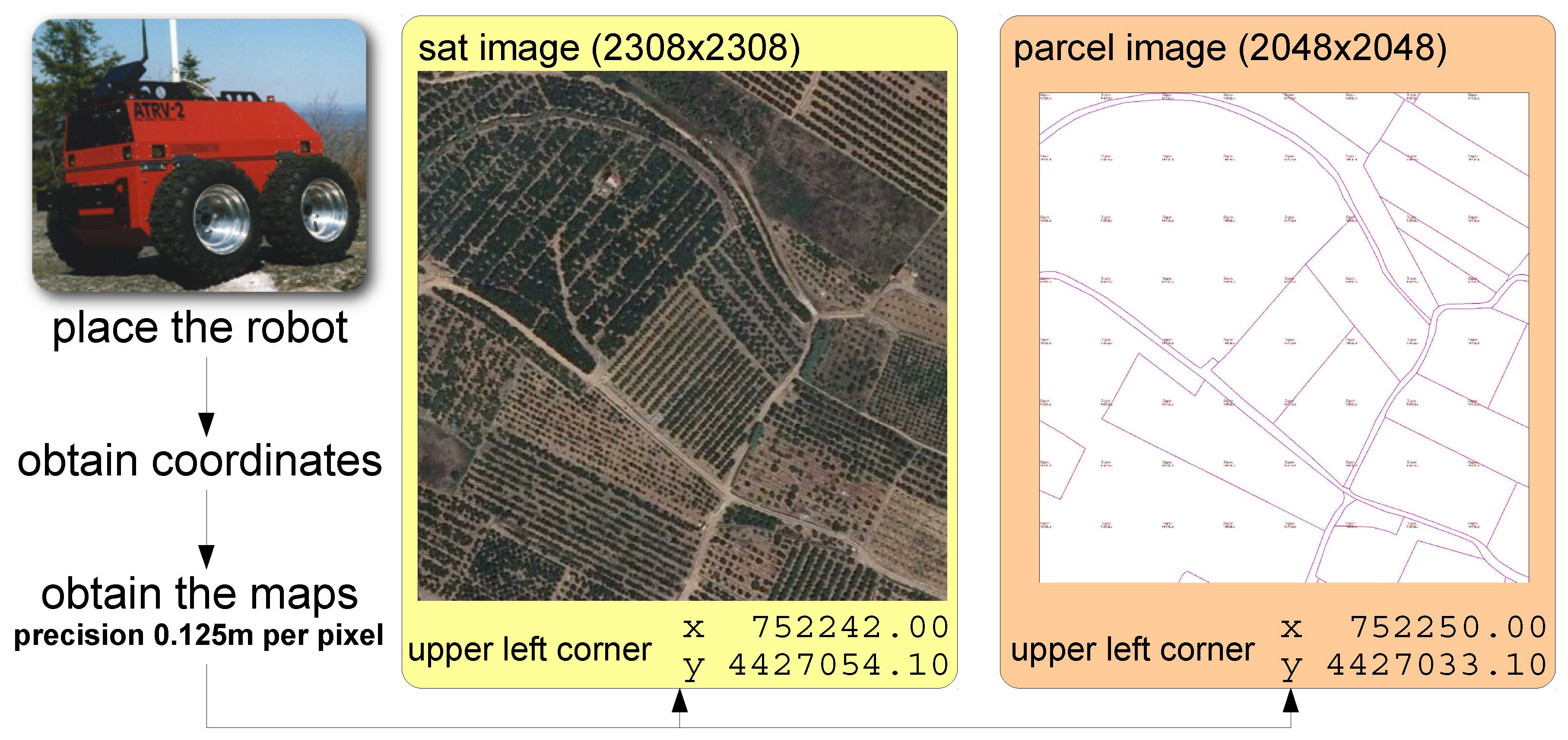
• Acquisition sub-module: This sub-module is in charge of acquiring the images from online databases to generate the final map of the parcel. Concretely, the system will download the images from a public administrative database, SIGPAC, using the information provided by the GPS sensor included in the robots. In other related experiments, we installed a submeter precision GPS in the autonomous robots (GPS Pathfinder ProXT Receiver) [22]. The location accuracy obtained in those cases encourages us to integrate that GPS in the current system. However, the GPS integration is out of this paper’s scope, since the main objective of this paper is to introduce the algorithms to combine satellite and cadastral images and to show a proof-of-concept. This sub-module provides two images to the “map creation module”: the satellite image of the parcel and the image with parcel borders.
• Map creation sub-module: This sub-module will be in charge of extracting all the information from the images: paths, orange trees, borders, and obstacles. With the extracted information, the map (path planning) which the robots should follow will be generated. The initial strategy to cover efficiently all the parcels with the robots will be done in this sub-module. The maps and satellite imagery resolution are set to 0.125 m per pixel. This resolution was easily reached with both services (satellite imagery and cadastral imagery) and was low enough to represent the robot dimensions (around 50 by 80 cm), and the computation burden was not so demanding. With the new Galileo services, higher resolution images can be obtained (with lower cm per pixel rates). Although more precise paths could be obtained, the computational cost of fast marching to generate the paths would also considerably increase.

3.1.1. Acquisition Sub-Module

This sub-module is in charge of obtaining the two images which are needed to create the map of the parcel from the current position of the autonomous system. Its description is detailed in Algorithm 1 where $CurrentPosition$ represents the current position of the robotic system, $Resolution$ is the resolution of the acquired imagery, and $Radius$ stands for the radius of the area.

Algorithm 1 ObtainImages{$CurrentPosition$,$Resolution$,$Radius$}

$FullSatImage$ = ObstainSatImage{$CurrentPosition$,$Resolution$,$Radius$} $Borders$ = ObstainBorders{$CurrentPosition$,$Resolution$,$Radius$} Return:$FullSatImage$, $Borders$

The output generated in this sub-module includes the full remote image of the area, $FullSatImage$, and the borders of the parcels, $Borders$, which will be processed in the “Map Creation module”.

3.1.2. Map Creation Sub-Module

This sub-module is in charge of creating the map of the parcel from the two images obtained in the previous sub-module. The map contains information about the parcel: trees rows, paths, and other elements where the robot cannot navigate through (i.e., obstacles). Its description can be found in Algorithm 2.

Algorithm 2 GenerateMap{$CurrentPosition$,$FullSatImage$,$Borders$}

$FullParcelMask$ = GenerateParcelMask{$CurrentPosition$,$Borders$} [$ParcelMask$,$SatImage$] = CropImagery{$FullParcelMask$,$FullSatImage$} [$Path$,$Trees$,$Obstacles$] = ExtractMasks{$CurrentPosition$,$ParcelMask$,$SatImage$}

The first step consists of determining the full parcel mask from the borders previously acquired. With the robot coordinates and the image containing the borders, this procedure generates a binary mask that represents the current parcel where the robot is located. This procedure is described in Algorithm 3.

Algorithm 3 GenerateParcelMask{$CurrentPosition$,$Borders$}

Determine position $CurrentPosition$ in $Borders$: $Po{s}_x$ and $Po{s}_y$ Convert $Borders$ to grayscale: $BordersG$ Binarize $BordersG$: $BordersMask$ Dilate $BordersMask$: $DilatedBorder$ Flood-fill $DilatedBorder$ in $Po{s}_x,Po{s}_y$: $DilatedBorderFloodfilled$ Erode $DilatedBorderFullfilled$: $ErodedBorderFloodfilled$ Dilate $ErodedBorderFloodfilled$: $FullParcelMask$ Return:$FullParcelMask$

Once the parcel mask is determined from the parcel image, it is time to remove those areas outside the parcel in the satellite image and the parcel mask itself. To avoid underrepresentation of the parcels, a small offset was added to the mask. This step is performed to reduce imagery size for further treatment with advanced techniques. This procedure is detailed in Algorithm 4.

Algorithm 4 CropImagery{$FullParcelMask$,$FullSatImage$}

Determine real position of left-upper corner of $FullParcelMask$ Determine real position of left-upper corner of $FullSatImage$ Determine $FullSatImage$ offset in pixels with respect $FullParcelMask$ Determine parcel’s bounding box:     Determine first and last row of $FullParcelMask$ that is in parcel     Determine first and last column of $FullParcelMask$ that is in parcel Crop $FullParcelMask$ directly: $ParcelMask$ Crop $FullSatImage$ according to offset values: $SatImage$ Return:$ParcelMask$ and $SatImage$

Since the location of the pixels in the real world is known using the WGS84 with UTM zone 30N system (EPSG:32630), the offset between the satellite image and the parcel mask can be directly computed. Then, it is only necessary to determine the bounding box surrounding the parcel in the parcel mask to crop both images.

At this point, the reduced satellite map needs to be processed to distinguish between the path and obstacles. We analyzed different satellite images from groves located in the province of Castellón in Spain, and the images were clear with little presence of shadows. Therefore, we set the binarization threshold to 112 in our work. Although we applied a manual threshold, a dynamic thresholding binarization could be applied to have a more robust method to distinguish the different elements in the satellite image, in case shadows were present. Algorithm 5 has been used to process the reduced satellite map andto obtain the following three masks or binary images:

• $Path$—a binary mask that contains the path where the robot can navigate;
• $Trees$—a binary mask that contains the area assigned to orange trees;
• $Obstacles$—a binary mask that contains those pixels which are considered obstacles: this mask corresponds to the inverse of the path.

Algorithm 5 GenerateMasks{$ParcelMask$ and $SatImage$}

Convert $SatImage$ to gray scale: $SatImageGray$ Extract $min$ and $max$ values of the parcel pixels in $SatImageG$ Normalize $SatImageG$ values:    $SatImageGN(x,y)=255·\frac{SatImageG(x,y)-MinValue}{MaxValue}$ Generate B&W Masks:         $\begin{array}{ll}Path(x,y)\hfill & =\left\{\begin{array}{ll}1& \mathrm{if}SatImageGN(x,y)>112\mathrm{and}ParcelMask(x,y)\\ 0& \mathrm{otherwise}\end{array}\right.\hfill \\ Trees(x,y)\hfill & =\left\{\begin{array}{ll}1& \mathrm{if}SatImageGN(x,y)\le 112\mathrm{and}ParcelMask(x,y)\hfill \\ 0& \mathrm{otherwise}\end{array}\right.\hfill \end{array}$ Remove path pixels not connected to $CurrentPosition$ in $Path$ Generate $Obstacles$ Mask:    $Obstacles(x,y)=1-Path(x,y)$ Return:$Path$$OrangeTrees$ and $Obstacles$

3.2. Second Stage: Path Planning

This module is used to determine the final path that the robotic system or team of robots should follow. The principal work for path planning in autonomous robotic systems is to search for a collision-free path and to cover all the groves. This section is devoted to describing all the steps necessary to generate the final path (see Algorithm 6) using as input the three masks provided by Algorithm 5.

To perform the main navigation task, the navigation module has been divided into five different sub-modules:

• Determining the tree lines
• Determining the reference points
• Determining the intermediate points where the robot should navigate
• Path planning through the intermediate points
• Real navigation through the desired path

First of all, the tree lines are determined. From these lines and the Path binary map, the reference points of the grove are determined. Later, the intermediate points are selected from the reference points. With the intermediate points, a fast path free of collisions is generated to cover all the groves. Finally, the robotic systems perform real navigation using the generated path.

Algorithm 6 PathPlanning{$CurrentPosition$,$Trees$,$Path$}

$SortedTreeLines$ = DetectLines{$Trees$,$Path$} [$Vertexes$,$MiddlePaths$] = ReferencePoints{$Path$,$SortedTreeLines$} $FinalPath$ = CalculatePath{$Position$,$Path$,$MiddlePath$,$Vertexes$ Return:$FinalPath$

3.2.1. Detecting Tree Lines

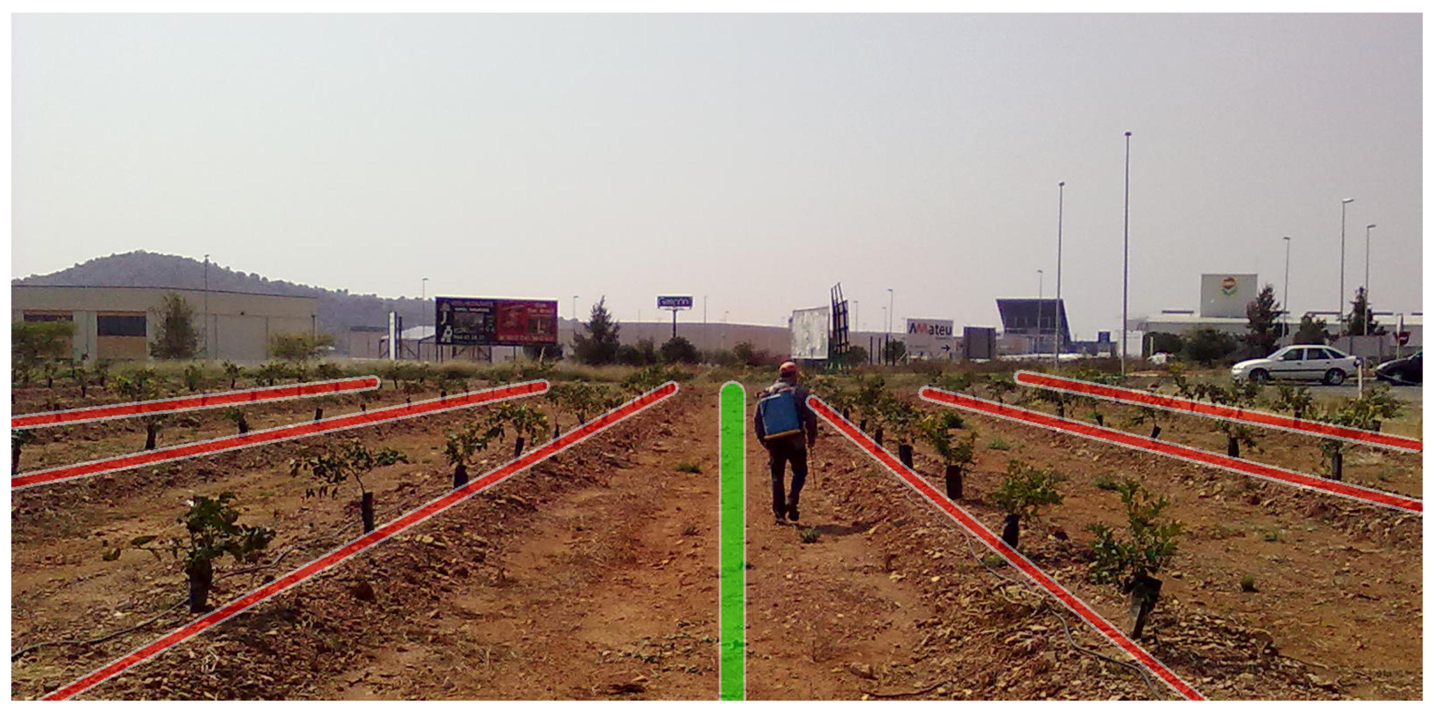
The organization of citric groves is well defined as it can be seen in the artificial composition depicted in Figure 2; the trees are organized in rows separated by a relatively wide path to optimize treatment and fruit collection. The first step of the navigation module consists of detecting the tree lines.

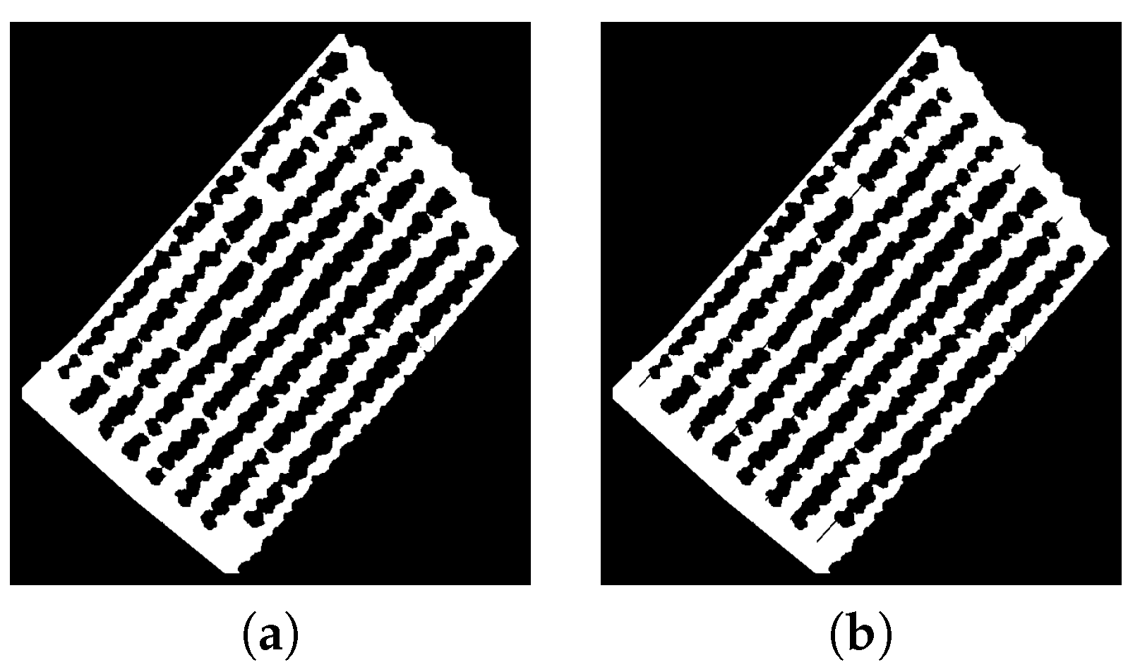
The Obstacles binary map ($Obstacles$ in Algorithm 5) contains the pixels located inside the parcel that correspond to trees. For this reason, the rows containing trees are extracted by using the Hough Transform method (see Reference [24]). Moreover, some constraints to this technique have been added to avoid selecting the same tree line several times. In this procedure, the Hesse standard form (Equation (1)) is used to represent lines with two parameters: $\theta$ (angle) and $\rho$ (displacement). Each element of the resulting matrix of the Hough Transform contains some votes which depend on the number of pixels which corresponds to the trees that are on the line.

$$y·sin\left({\theta }_{path}\right)+x·cos\left({\theta }_{path}\right)-{\rho }_{path}=0$$

(1)

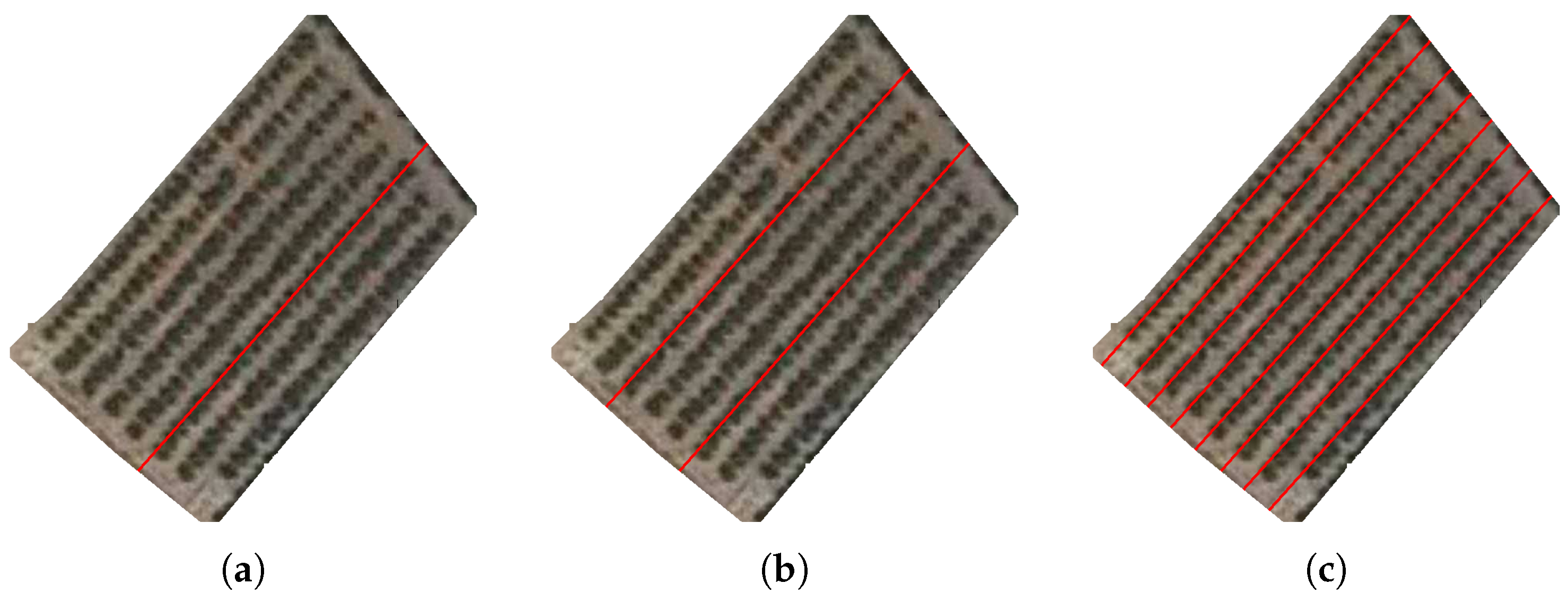
According to the structure of the parcels, the main tree rows can be represented with lines. We applied Algorithm 7 to detect the main tree rows (rows of citric trees). First, the most important lines, the ones with the highest number of votes, are extracted. The first extracted line (the line with the highest number of votes) is considered the “main” line, and its parameters (${\theta }_1$, ${\rho }_1$ and $vote{s}_1$) are stored. Then, those lines that have at least $0.20·vote{s}_1$ and of which the angle is $\rho \pm 1.5$ are also extracted. This first threshold (${\Gamma }_1=0.20$) has been used to filter the small lines that do not represent full orange rows, whereas the second threshold (${\Gamma }_2=1.5$) has been used to select those orange rows parallel to the main line. We have determined the two threshold values according to the characteristics of the analyzed groves: the target groves have parallel orange rows with similar length.

Algorithm 7 DetectLines{$Trees$,$Path$}

Apply $Hough$ to $Threes$: $H=Hough\left(Trees\right)$ Extract line with highest value from H: $valu{e}_{main}=H({\rho }_{main}$,${\varphi }_{main}$) Set Treshold value: ${\Gamma }_1=0.20·valu{e}_{main}$ Limit H to angles close the main angle (${\varphi }_{main}\pm {1.5}^{\circ }$): $HL$ lines = true Store main line parameters in $StoredLines$: ${\rho }_{main}$ ${\varphi }_{main}$ $valu{e}_{main}$ while lines do  Extract candidate line with highest value from $HL$: $valu{e}_c=HL({\rho }_c$,${\varphi }_c$)  Remove value in the matrix: $HL({\rho }_c,{\varphi }_c)=0$  if ($valu{e}_c>{\Gamma }_1$) then   Calculate that distance to previous extracted lines is lower than threshold:      $\parallel {\rho }_c-{\rho }_i\parallel >(12·(1+\parallel {\theta }_c-{\theta }_i\parallel \left)\right)$   if distance between candidate and stored lines is never lower than threshold then    Store line parameters in $StoredLines$: ${\rho }_c$ ${\varphi }_c$ $valu{e}_c$   end if  else   lines = false  end if end while Sort stored lines: $SortedTreeLines$ Return:$SortedTreeLines$

Furthermore, to avoid detecting several times the same tree row, each extracted line cannot be close to any previous extracted line. We used Equation (2) to denote the distance between a candidate line (c) and a previous extracted line (i) since the angles are similar ($\pm {1.5}^{\circ }$). If this distance is higher than a threshold value (${\Gamma }_3$), the candidate line is extracted. We use Equation (3) to calculate the threshold value according to the difference of angles of the two lines.

$$distanc{e}_{c,i}=\parallel {\rho }_c-{\rho }_i\parallel$$

(2)

$${\Gamma }_3=12·(1+\parallel {\theta }_c-{\theta }_i\parallel )$$

(3)

Hough Transform has been commonly used in the literature related to detection tasks in agricultural environments. Recent research shows that it is useful to process local imagery [25,26] and remote imagery [27,28].

3.2.2. Determining the Reference Points

Reference or control points contain well-known points and parts of the grove, e.g., the vertex of the orange tree lines or the middle of paths where farmers walk. A set of reference points will be used as intermediate points in the entire path that a robotic system should follow.

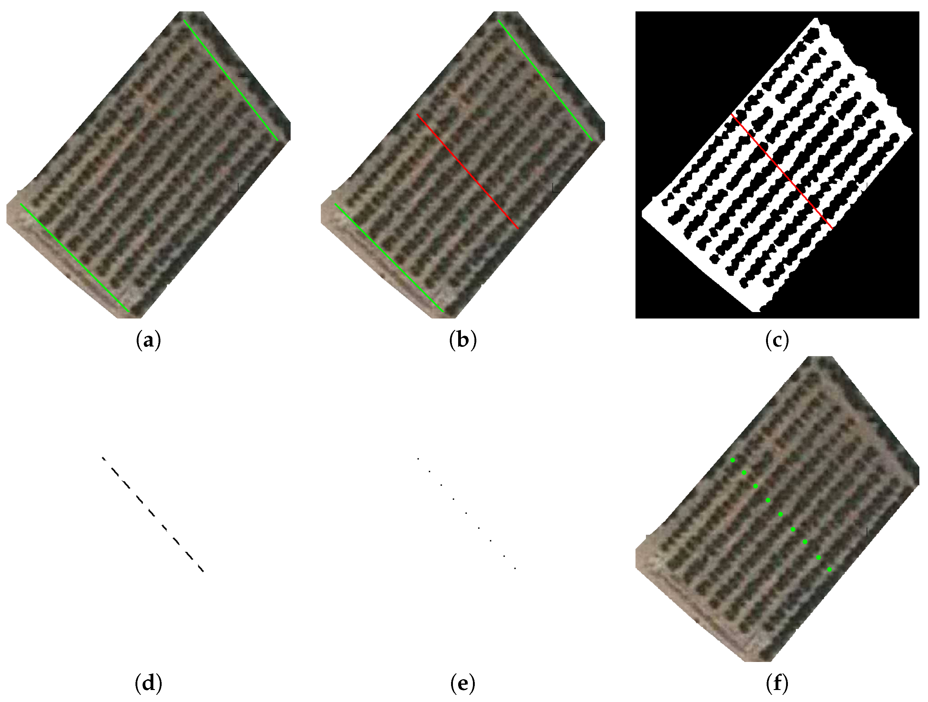
Firstly, the vertexes of the orange tree rows are extracted. For each extracted line, the vertexes correspond to the first and last points that belongs to the path according to the Path binary map $Path$.

Then, Hough transform is applied again to detect the two border paths perpendicular to the orange rows. With these two lines, their bisection is used to obtain additional reference points. These last points correspond to the centre of each path row (the path between two orange rows). Concretely, the intersection between the bisection line and the Path binary map is used to calculate the points. After obtaining the intersection, the skeleton algorithm is applied to obtain the precise coordinates of the new reference points.

However, under certain conditions, two central points have been detected for the same row, e.g., if obstacles are present at the centre of the path, the skeleton procedure can provide two (or more) middle points between two orange tree rows. In those cases, only the first middle point is selected for each path row.

Finally, all the reference points can be considered basic features of the orange grove since a subset of them will be used as intermediate points of the collision-free path that a robotic system should follow to efficiently navigate through the orange grove. For that purpose, we applied Algorithm 8 to extract all the possible middle points in a parcel.

Algorithm 8 ReferencePoints{$Path$ $SortedTreeLines$}

$Vertexes$ = Extract reference points from $SortedTreeLines$ $MiddlePaths$ = Extract reference points that belong to middle of path rows Return:$Vertexes$ and $MiddlePaths$

3.2.3. Determine Navigation Route from Reference Points

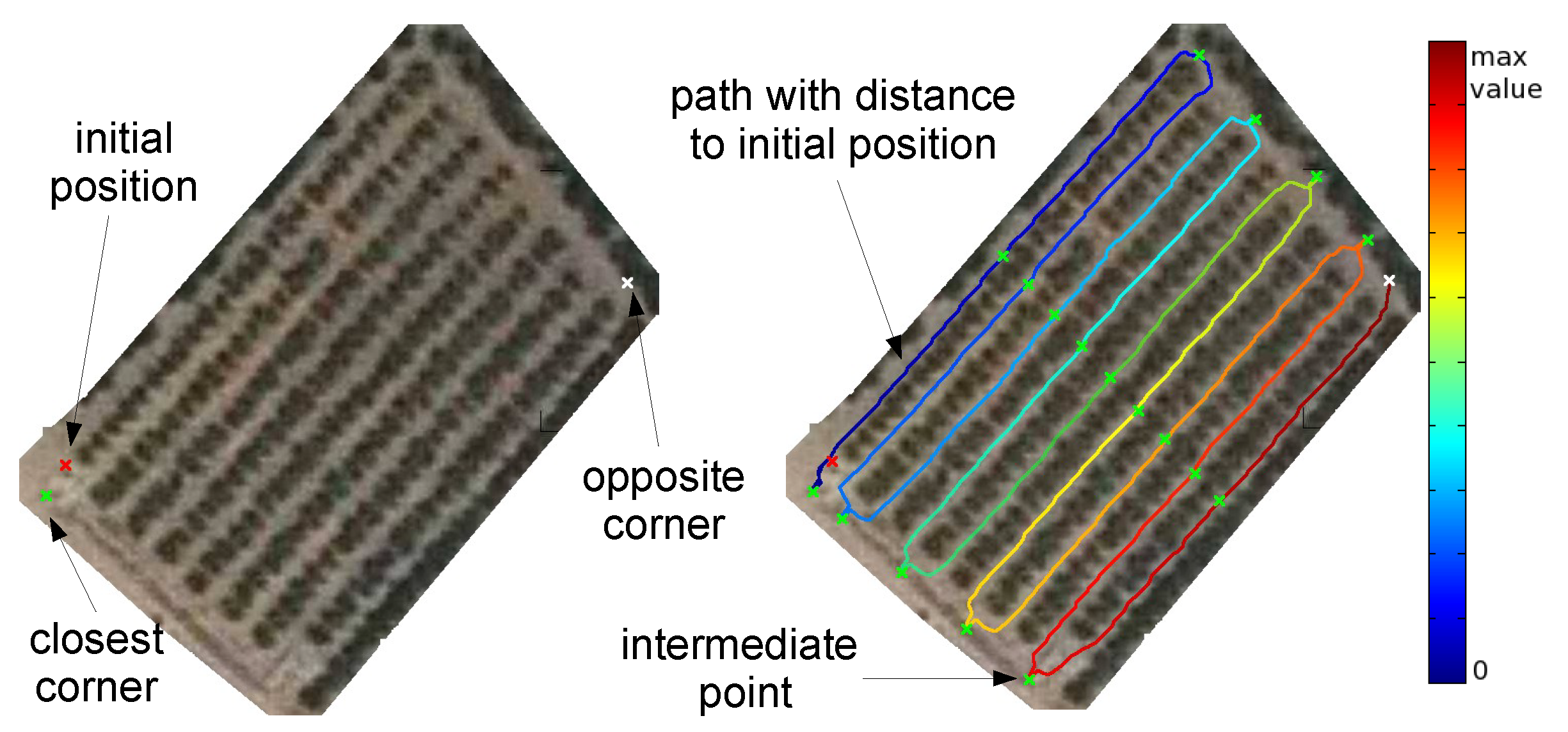
In this stage, the set with the intermediate points is extracted from the reference points. They correspond to the points where the robot should navigate. The main idea is first to move the robot to the closest corner, and then, the robot navigates through the grove (path row by path row), alternating the direction of navigation (i.e., a zig-zag movement).

Firstly, the closest corner of the parcel is determined by the coordinates provided by the robotic system using the Euclidean distance. The corners are the vertexes of the lines extracted from the first and last rows containing trees previously detected. The idea is to move the robot from one side of the parcel to the opposite side through the row paths. The sequence of intermediate points is generated according to the first point (corner closest to the initial position of the robot) being the opposite corner the destination. Intermediate points are calculated using Algorithm 9.

Finally, this stage is not directly performed by path planning but Algorithm 10) will be used to determine the sequence of individual points. Those points will be the basis for the next stage where the paths for any robotic system that composes the team are determined.

Algorithm 9 IntermediatePoints{$Position$,$MiddlePaths$,$Vertexes$}

Extract corners from $Vertexes$:   $Corners$ = [$Vertexes\left(1\right)$,$Vertexes\left(2\right)$,$Vertexes\left(Penultimate\right)$,$Vertexes\left(Last\right)$] Detect closest corner to $CurrentPosition$: $Corner$ Add $Corner$ to $ListIntermediatePoints$ $ListPoints=SequencePoints\{Corner,MiddlePaths,Vertexes\}$ Add $ListPoints$ to $ListIntermediatePoints$ Return:$ListIntermediatePoints$

Algorithm 10 SequencePoints{$Corner$,$MiddlePaths$,$Vertexes$}

Let be $N_{points}$ the number of points in $MiddlePath$ if$Corner$ is $Vertexes\left(1\right)$ then  for i = 1 to ($N_{points}$-1) do   Add MiddlePaths(i) to $ListPoints$   Add $Vertexes(i·2-module(i+1,2\left)\right)$ to $ListIPoints$  end for  Add MiddlePaths($N_{points}$) to $ListPoints$  Add Vertexes($last$) to $ListPoints$ end if if$Corner$ is $Vertexes\left(2\right)$ then  for i = 1 to ($N_{points}$-1) do   Add MiddlePaths(i) to $ListPoints$   Add $Vertexes(i·2-module(i,2\left)\right)$ to $ListPoints$  end for  Add MiddlePaths($N_{points}$) to $ListPoints$  Add Vertexes($penultimate$) to $ListPoints$ end if if$Corner$ is $Vertexes\left(penultimate\right)$ then  for i = 1 to ($N_{points}$-1) do   $j=N_{points}+1-i$   Add MiddlePaths(j) to $ListIPoints$   Add $Vertexes\left(\right(j-1)·2-module(i,2\left)\right)$ to $ListPoints$  end for  Add MiddlePaths(1) to $ListPoints$  Add Vertexes(2) to $ListPoints$ end if if$Corner$ is $Vertexes\left(last\right)$ then  for i = 1 to ($N_{points}$-1) do   $j=N_{points}+1-i$   Add MiddlePaths(j) to $ListPoints$   Add $Vertexes\left(\right(j-1)·2$ - module(i+1,2)) to $ListPoints$  end for  Add MiddlePaths(1) to $ListPoints$  Add Vertexes(1) to $ListPoints$ end if Return:$ListPoint$

3.2.4. Path Planning Using Processed Satellite Imagery

Once the initial and intermediate points and their sequence are known, the path planning map is determined. This means calculating the full path that the robotic system should follow.

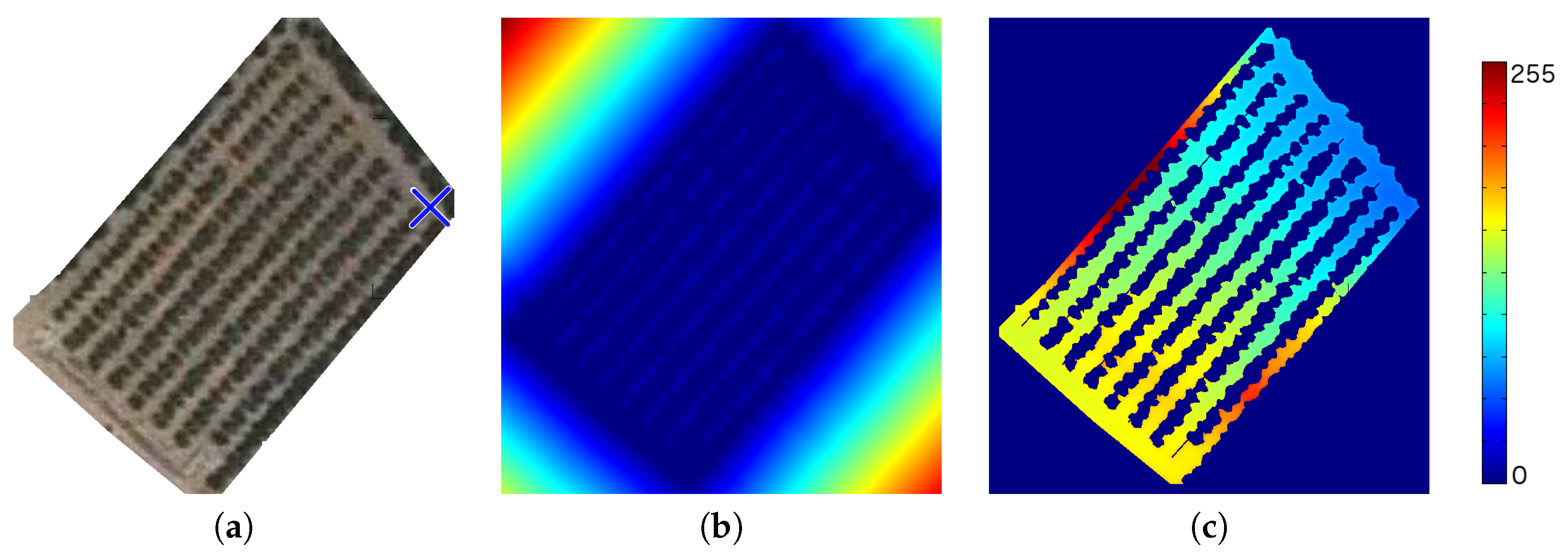
Firstly, the $Speed$ map is calculated with Equation (4). This map is related to the distance to the obstacles (where the robot cannot navigate). The novel equation introduces a parameter, $\alpha$, to penalize those parts of the path close to obstacles and to give more priority to those areas which are far from obstacles. Theoretically, the robotic system will navigate faster in those areas far from obstacles due to the low probability of collision with the obstacles. Therefore, the equation has been chosen to penalize the robotic system for navigating close to obstacles.

$$Speed(x,y)=\left\{\begin{array}{cc}100+distance{(x,y)}^{\alpha }& \mathrm{if}distance(x,y)>0\\ 1& \mathrm{otherwise}\end{array}\right.$$

(4)

where $distance$ refers to the pixel-distance of point $(x,y)$ in the image to the closest obstacle. The final $Speed$ value is set to value 1 when the pixel corresponds to an obstacle, whereas it has a value higher than 100 in those pixels which correspond to the class “path”.

The final procedure carried out to calculate the $Speed$ image is detailed in Algorithm 11.

Algorithm 11$Speed$ = CalculateSpeed{$Path$, $SortedTreeLines$}

Add detected tree lines to the path binary mask $Path$ Select Non-Path points with at least one neighbor which belong to path: $ObstablePoints$ Set initial $Speed$ values: $Speed(x,y)=1$∀$x\in [1,TotalWidth]$ $y\in [1,TotalHeight]$ for x=1:$TotalWidth$ do  for y=1:$TotalHeight$ do   if PathMask(x,y) belongs to Path then    Calculate Euclidean distance to all ObstaclePoints    Select the lowest distance value: $mindistance$    $Speed(x,y)=100+mindistanc{e}^3$   end if  end for end for Return:$Speed$

Then, the Fast Marching algorithm is used to calculate the $Distances$ matrix. It contains the “distance” to a destination for any point of the satellite image. The values are calculated using the $Speed$ values and the target/destination coordinates in the satellite image. The result of this procedure is a $Distance$ matrix of which the normalization can be directly represented as an image. This distance does not correspond to the Euclidean distance; it corresponds to a distance measurement based on the expected time required to reach the destination.

The Fast Marching algorithm, introduced by Sethian (1996), is a numerical algorithm that is able to catch the viscosity solution of the Eikonal equation. According to the literature (see References [29,30,31,32,33]), it is a good indicator of obstacle danger. The result is a distance image, and if the speed is constant, it can be seen as the distance function to a set of starting points. For this reason, Fast Marching is applied to all the intermediate points using the previously calculated distances as speed values. The aim is to obtain one distance image for each intermediate point; this image provides information to reach the corresponding intermediate point from any other point of the image.

Fast Marching is used to reach the fastest path to a destination, not the closest one. Although it is a time-consuming procedure, an implementation based on MultiStencils Fast Marching [34] has been used to reduce computational costs and to use it in real-time environments.

The final $Distances$ matrix obtained is used to reach the destination point from any other position of the image with an iterative procedure. The procedure carried out to navigate from any point to another determined point is given by Algorithm 12. First, the initial position (position where the robotic system is currently placed) is assigned to the path; then, the algorithm seeks iteratively for the neighbour with lowest distance value until the destination is reached ($Distance$ value equal to 0). This algorithm will provide the path as a sequence of consecutive points (coordinates of the distance image). Since the geometry of the satellite imagery is well known, the list of image coordinates can be directly translated to real-world coordinates. This information will be used by the low-level navigation system to move the system according to the calculated path.

Algorithm 12$PathPoints$ = NavigationPt2Pt{$InitialPt$,$DestinyPt$,$Speed$}

$Distances=FastMarching(DestinyPt,Speed)$ $CurrentPoint=InitialPt$ while$Distances(Currentpoint.x,Currentpoint.y)>0$do  Search the neighbor with lowest Distance Value: $NewPoint$  $CurrentPoint=NewPoint$  Add $CurrentPoint$ to $PathPoints$ end while Return:$PathPoints$

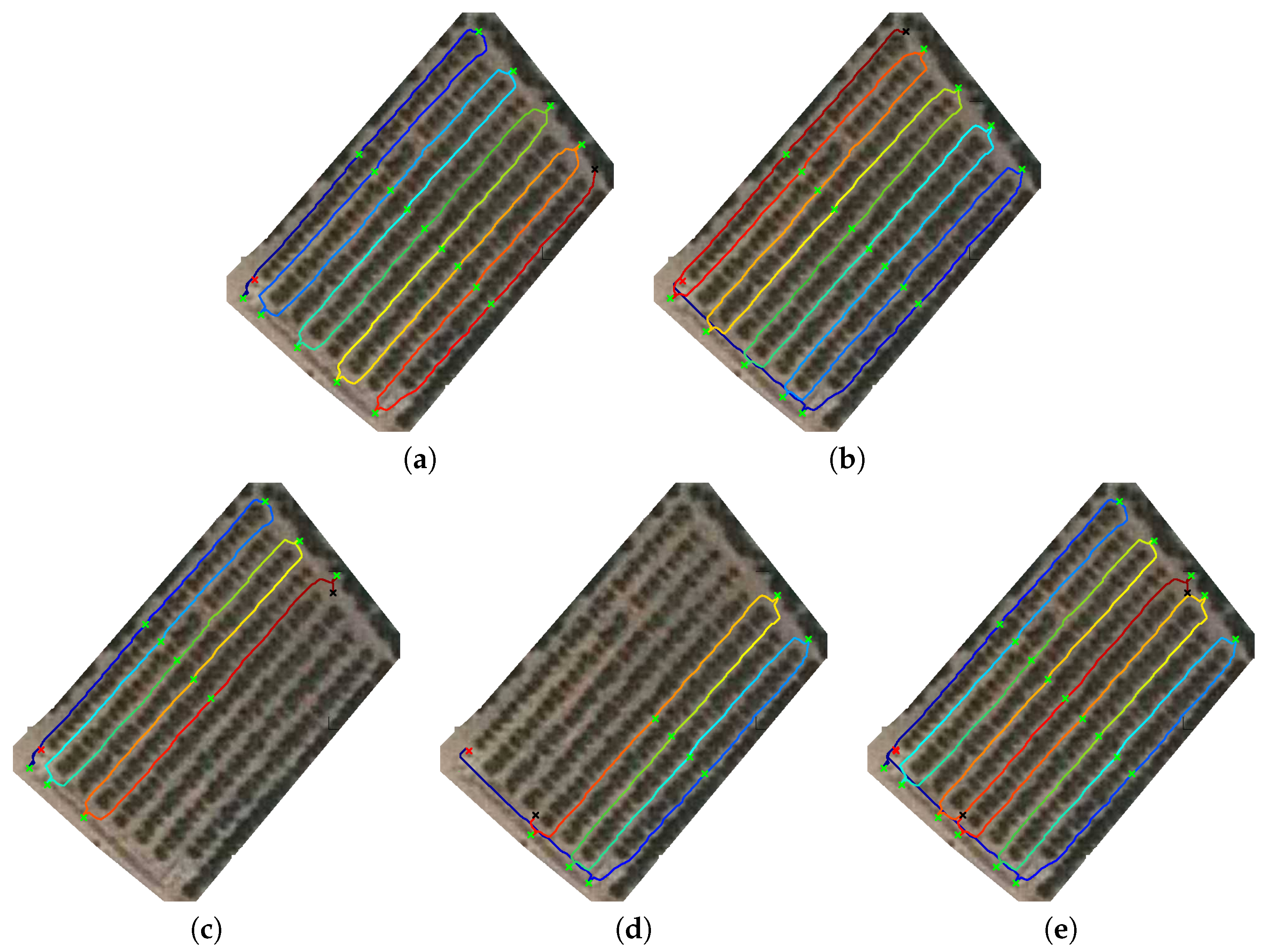
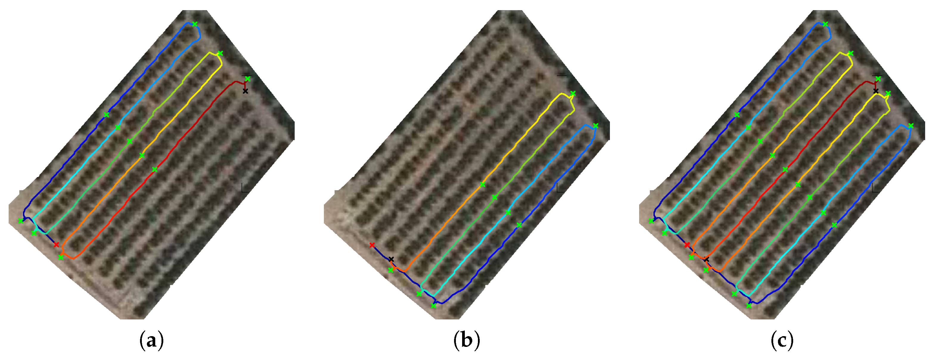
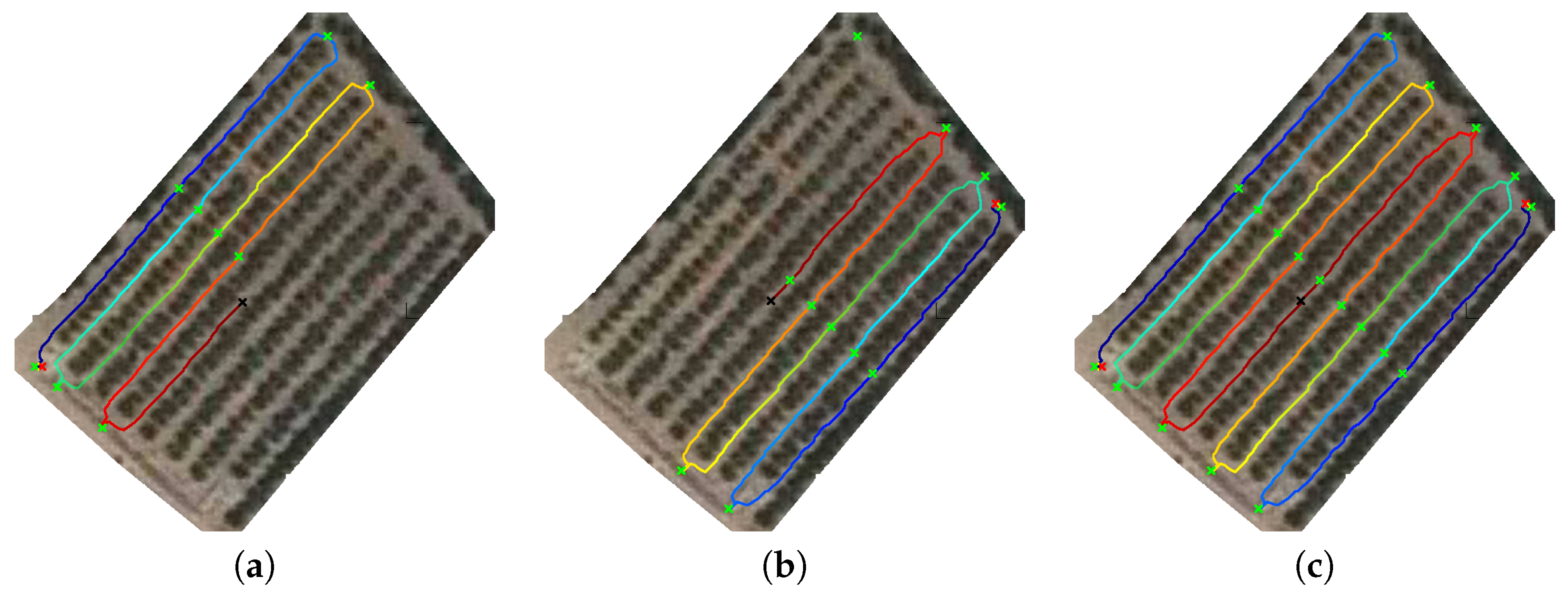
Finally, the final full path that the robotic system should follow consists of reaching sequentially all the intermediate points previously determined. This strategy is fully described in Algorithm 13, but it is only valid for the case of using only one single robotic system in the grove. For more than one robot present in the grove, an advanced algorithm is needed. Algorithm 14 introduces the strategy for two robots when they are close to each other.

Algorithm 13 CalculatePath{$Position$,$Path$,$MiddlePaths$,$Vertexes$}

$ListPoints=SequencePoints\{CurrentPosition,MiddlePaths,Vertexes\}$ $Speed=CalculateSpeed\left(Path\right)$ $StartingPoint$ = $CurrentPosition$ for i = 1 to NumberOfIntermediatePoints do  $IntermediatePoint=ListPoints\left(i\right)$  $PathPoints=NavigationPt2Pt\{$ $StartingPoint$,$IntermediatePoint$,$Speed$}  Add $PathPoints$ to $FinalPath$  $StartingPoint=IntermediatePoint$ end for Return:$FinalPath$

Algorithm 14 CalculatePath{$Positions$,$Path$,$MiddlePaths$,$Vertexes$}

Extract current position for robot 1: $CurrentPosition{s}_{robot1}$ Extract current position for robot 2: $CurrentPosition{s}_{robot2}$ Extract corners from $Vertexes$:   $Corners$ = [$Vertexes\left(1\right)$,$Vertexes\left(2\right)$,$Vertexes\left(Penultimate\right)$,$Vertexes\left(Last\right)$] Detect closest corner and the distance for the two robots   $Corne{r}_{robot1}=getClosestCorner(CurrentPosition{s}_{robot1},Corners)$   $distanc{e}_{robot1}=getPixelDistance(CurrentPosition{s}_{robot1},Corne{r}_{robot1})$   $Corne{r}_{robot2}=getClosestCorner(CurrentPosition{s}_{robot2},Corners)$   $distanc{e}_{robot2}=getPixelDistance(CurrentPosition{s}_{robot2},Corne{r}_{robot2})$ if$distanc{e}_{robot1}<distanc{e}_{robot2}$then  Add $Corne{r}_{robot1}$ to $ListIntermediatePoin{t}_{robot1}$  $ListPoint{s}_{robot1}=SequencePoints\{Corne{r}_{robot1},MiddlePaths,Vertexes\}$  Add $ListPoint{s}_{robot1}$ to $ListIntermediatePoin{t}_{robot1}$  Detect opposite corner to $Corne{r}_{robot1}$ closest to robot 2: $Opposit{e}_{robot1}$  Add $Opposit{e}_{robot2}$ to $ListIntermediatePoin{t}_{robot2}$  $ListPoint{s}_{robot2}=SequencePoints\{Opposit{e}_{robot2},MiddlePaths,Vertexes\}$  Add $ListPoint{s}_{robot2}$ to $ListIntermediatePoin{t}_{robot2}$ else  Add $Corne{r}_{robot2}$ to $ListIntermediatePoin{t}_{robot2}$  $ListPoint{s}_{robot2}=SequencePoints\{Corne{r}_{robot2},MiddlePaths,Vertexes\}$  Add $ListPoint{s}_{robot2}$ to $ListIntermediatePoin{t}_{robot2}$  Detect opposite corner to $Corne{r}_{robot2}$ closest to robot 1: $Opposit{e}_{robot1}$  Add $Opposit{e}_{robot1}$ to $ListIntermediatePoin{t}_{robot1}$  $ListPoint{s}_{robot1}=SequencePoints\{Opposit{e}_{robot1},MiddlePaths,Vertexes\}$  Add $ListPoint{s}_{robot1}$ to $ListIntermediatePoin{t}_{robot1}$ end if $Speed=CalculateSpeed\left(ParcelMask\right)$ $StartingPoin{t}_{robot1}$ = $CurrentPositio{n}_{robot1}$ for i = 1 to NumberOfIntermediatePoints do  $IntermediatePoint=ListIntermediatePoints\left(i\right)$ f  $Path=NavigationPoint2Point\{$ $StartingPoint$,$IntermediatePoint$,$Speed$}  Add $Path$ to $FinalPat{h}_{robot1}$  $StartingPoint=IntermediatePoint$ end for $StartingPoin{t}_{robot2}$ = $CurrentPositio{n}_{robot2}$ for i = 1 to NumberOfIntermediatePoints do  $IntermediatePoint=ListIntermediatePoints\left(i\right)$  $Path=NavigationPoint2Point\{$ $StartingPoint$,$IntermediatePoint$,$Speed$}  Add $Path$ to $FinalPat{h}_{robot2}$  $StartingPoint=IntermediatePoint$ end for Store $FinalPath$

4. Results on a Real Case: Proof-of-Concept Validation

The previous section introduced the algorithms to obtain the path that a robot or system of two robots have to follow to cover the whole citric grove for, for instance, maintenance tasks. To show the feasibility of the proposed system, the system has been evaluated in a real context as a proof-of-concept.

4.1. Results of the Mapping System

First, given the current position of the robot (or team of robots), the maps and parcel masks are obtained. For our test, a GPS receiver with submeter precision was used. It is important to remark that the system must be inside the parcel to get the data accurately. From the initial position of the system, inside the parcel, the satellite maps of the parcel will be obtained using a satellite maps service via the Internet. In our case, two images were downloaded from the SIGPAC service, the photography of the parcel and the image with the boundaries of the parcel, as can be seen in Figure 3. Due to the characteristics of the latter image, some additional steps were included in Algorithm 3.

In Algorithm 3, the image with the borders of the parcel (see parcel image in Figure 3) is first processed to obtain a binary mask with pixels which belongs to the parcel and the pixels which are outside the parcel. For this reason, this image is first converted to black and white with a custom binarization algorithm (see Figure 4a). The purpose of the binarization is double: (1) to remove watermarks (red pixels in Figure 3) and (2) to highlight the borders (purple pixels in Figure 3).

This early version of the binary mask is then dilated to perform a better connection between those pixels which correspond to the border (see Figure 4b). The dilation is performed three times with a 5 × 5 mask. Then, the pixel corresponding to the position of the robots is flood-filled in white (see Figure 4c). Finally, the image is eroded to revert the dilated filtering previously performed and to remove the borders between parcels. For this purpose, the erosion algorithm is run 6 times with the same 5 × 5 mask. After applying this last filter, the borders are removed and the parcel area is kept in the mask image. After obtaining the last binary mask, it is dilated again 3 times to better capture the real borders of the parcel (see Figure 4d).

Then, it is only necessary to determine the bounding box surrounding the parcel in the parcel mask (see Figure 4d) to crop both images. This procedure is visually depicted on the top side of Figure 5.

The first mask, $Path$, contains the path where the robot can navigate (see Figure 5b). The second mask, $Trees$, contains the area assigned to orange trees (see Figure 5c). The last mask, $Obstacles$, contains those pixels which are considered obstacles; this mask corresponds to the inverse of the path (see Figure 5d).

4.2. Results of the Path Planner System

4.2.1. Detecting Tree Lines

As a result of the Hough Transform application in Algorithm 7, all the orange tree rows are extracted as depicted in Figure 6. Although the order in which they are extracted does not correspond to the real order inside the grove, they are reordered and labelled according to its real order for further steps.

4.2.2. Determining the Reference Points

Algorithm 8 introduced how to determine the reference points that could be used as intermediate points in the path planner. Figure 7 and Figure 8 show a graphical example of these reference points. The former set of images shows how the tree row vertexes are computed, whereas the latter includes the process to extract the middle point of each path row.

4.2.3. Determine Navigation Route from Reference Points

The results of Algorithm 9 are shown in Figure 9, where the numbered sequence of points is shown for four different initial configurations. In each one, the robot is placed near a different corner, simulating four possible initial places for the robots, so the four possible intermediate point distributions are considered.

4.2.4. Path Planning Using Processed Satellite Imagery

Algorithm 11 is used to calculate the $Speed$ image required to determine the path that the robot should follow. Initially, the Path binary map (Figure 10a) was considered to be used as a base to determine the distances, but a modified version was used instead (Figure 10b). The modification consisted of adding the detected lines for the orange rows. The lines have been added to ensure that the robot navigates entirely through each path row and that there is no way of trespassing the orange tree rows during navigation.

Three different $Speed$ images are shown in Figure 11a–c depending on the value of the $\alpha$ parameter. After performing some experiments, the best results are obtained when the $\alpha$ value is set to 3. With lower values of $\alpha$, the points close to obstacles were not penalized. With higher values, some narrow path rows were omitted from navigation due to their low-speed values. Finally, in our experiments, we used $\alpha =3$, as shown in Algorithm 11.

Figure 12a shows the parcel with the destination position drawn on it along with two representations of the $Distances$ matrix (Figure 12b,c). The first one corresponds to the normalized $Distances$ matrix of which the values are adapted to the $[0\dots 255]$ range. However, it is nearly impossible to visually see how to arrive at the destination from any other point inside the parcel. It is due to the high penalty value assigned to those points belonging to obstacles (non-path points). For this reason, a modified way to visualize the distance matrix is introduced by the following equation:

$$DistImg(x,y)=\left\{\begin{array}{cc}100+155\frac{Distances(x,y)}{max\left(Distances\right)}\hfill & \mathrm{if}Obstacles(x,y)=false\hfill \\ 0\hfill & \mathrm{otherwise}\hfill \end{array}\right.$$

(5)

In the image, it can be seen that there are high distance values in the first and last path rows (top-left and bottom-right sides of Figure 12c) which are not present in most of the other path rows. These two rows are narrow, and the speed values are, therefore, also quite low. For example, a robot placed in the top-left corner should navigate through the second path row to achieve the top-right corner instead of navigating through the shortest path (first path row). The aim of Fast Marching is to calculate the fastest path to achieving the destination point, not the shortest one. In the first row, the distance to obstacles is almost always very low.

Figure 13 shows the results of the path planner for a robotic system. In the example image, the robotic is initially placed in the location marked with the red x-cross. Then, all the intermediate points, including the closest corner, are determined (green x-crosses).

Figure 14 introduces an example for a team composed of two robots. Figure 14a,b shows the complete determined path for the first and second robots. The first robot moves to the closest corner and then navigates through the grove, and the second robot moves to the closest opposite corner (located at the last row) and then also navigates through the grove but in the opposite direction (concerning the first robot). The path is coloured depending on the distance to the initial position (blue is used to denote low distances, and red is used to denote high distances).

However, the robotic systems will not perform all the paths because they will arrive at a point (stop point marked with a black x-cross) which has been already reached by the other robotic system and they will stop there (see Figure 14c,d). The colour between the initial point (red x-cross) and the stop point (black x-cross) graphically denotes the relative distance. Finally, Figure 14d shows a composition of the path done by each robotic system into one image.

Similar examples are shown in Figure 15 and Figure 16, where the robots are not initially close to the corners. In the former example, the path between the initial position and the corners are not marked as “visited” because the robotic system navigation starts when the robot gets to the first intermediate point. In the latter case, we show an example where the robots stop when they detect that they have reached the same location.

5. Conclusions

This paper has shown a proof-of-concept of a novel path planning based on remote imagery publicly available. The partial results, shown as intermediate illustrative real examples of each performed step, encourage reliance on satellite imagery and cadastral information to automatically generate the path planning. According to it, useful knowledge can be obtained from the combination of satellite imagery and information about the borders that divide the land into parcels. Some limitations have been also identified: some parameters (such as thresholds) are image dependent and have been manually set for the current set of satellite images; it can only be applied in the current configuration of citric trees in rows; and changes in the grove distribution are not immediately reflected in the satellite imagery. In our platform, this path planning is complemented by local imagery, which provides navigation centred in the path.

We can conclude by remarking that the steps necessary to autonomously determine path planning in citric groves in the province of Castellón have been described in this paper and that the potential of this autonomous path planner has been shown with successful use cases. Firstly, a procedure to extract binary maps from a public remote imagery service has been described. Secondly, a novel methodology to automatically detect reference points from orange groves has been introduced using remote imagery. Some knowledge and global information about the grove can be extracted from those points. Thirdly, a procedure to determine a path has been designed for a stand-alone robotic vehicle. Moreover, it has been modified to be suitable for a team composed of two robotic systems. The first path planning provides useful information, and it may be considered the fast way to perform a maintenance task. This path is complemented by local navigation techniques (see Reference [21]) to obtain optimal results in the final implementation of the whole navigation module. Finally, although we introduced the system for orange groves, all the steps can be applied to other groves with a similar main structure (other citrus groves or some olive groves). Moreover, they could be also adapted for other crops or situations by changing the way they extract reference points, i.e., a hybrid team of multiple robots will require a specific planner and path strategy.

Finally, this paper has introduced a proof-of-concept showing the feasibility of the proposed algorithms to automatically determine path planning inside a citric grove. The proposed algorithms can be used to ease the manual labelling of satellite imagery to create manual maps for each parcel. We will identify the full implementation in different contexts and experimental validation as further work.

References

1. Blazquez, C.H.; Edwards, G.J.; Horn, F.W. Citrus grove mapping with colored infrared aerial photography. Proc. Fla. State Hortic. Soc. 1979, 91, 5–8. [Google Scholar]
2. López-Granados, F. Weed detection for site-specific weed management: Mapping and real-time approaches. Weed Res. 2011, 51, 1–11. [Google Scholar] [CrossRef]
3. Amorós López, J.; Izquierdo Verdiguier, E.; Gómez Chova, L.; Muñoz Marí, J.; Rodríguez Barreiro, J.; Camps Valls, G.; Calpe Maravilla, J. Land cover classification of VHR airborne images for citrus grove identification. ISPRS J. Photogramm. Remote Sens. 2011, 66, 115–123. [Google Scholar] [CrossRef]
4. Peterson, D.; Wolford, S. Fresh-market quality tree fruit harvester. Part II: Apples. Appl. Eng. Agric. 2003, 19, 545–548. [Google Scholar]
5. Arima, S.; Kondo, N.; Monta, M. Strawberry Harvesting Robot on Table-Top Culture; Technical Report; American Society of Association Executives (ASAE): St. Joseph, MI, USA, 2004. [Google Scholar]
6. Hannan, M.; Burks, T. Current Developments in Automated Citrus Harvesting; Technical Report; American Society of Association Executives (ASAE): St. Joseph, MI, USA, 2004. [Google Scholar]
7. Foglia, M.; Reina, G. Agricultural Robot Radicchio Harvesting. J. Field Robot. 2006, 23, 363–377. [Google Scholar] [CrossRef]
8. Blasco, J.; Aleixos, N.; Roger, J.; Rabatel, G.; Moltó, E. Robotic weed control using machine vision. Biosyst. Eng. 2002, 83, 149–157. [Google Scholar] [CrossRef]
9. Bak, T.; Jakobsen, H. Agricultural robotic platform with four wheel steering for weed detection. Biosyst. Eng. 2004, 87, 125–136. [Google Scholar] [CrossRef]
10. Downey, D.; Giles, D.; Slaughter, D. Weeds accurately mapped using DGPS and ground-based vision identification. Calif. Agric. 2004, 58, 218–221. [Google Scholar] [CrossRef]
11. Giles, D.; Downey, D.; Slaughter, D.; Brevis-Acuna, J.; Lanini, W. Herbicide micro-dosing for weed control in field grown processing tomatoes. Appl. Eng. Agric. 2004, 20, 7355–7743. [Google Scholar] [CrossRef]
12. Xiang, H.; Tian, L. Development of a low-cost agricultural remote sensing system based on an autonomous unmanned aerial vehicle (UAV). Biosyst. Eng. 2011, 108, 174–190. [Google Scholar] [CrossRef]
13. Dalponte, M.; Bruzzone, L.; Gianelle, D. Tree species classification in the Southern Alps based on the fusion of very high geometrical resolution multispectral/hyperspectral images and LiDAR data. Remote Sens. Environ. 2012, 123, 258–270. [Google Scholar] [CrossRef]
14. Stentz, A.; Dima, C.; Wellington, C.; Herman, H.; Stager, D. A System for Semi-Autonomous Tractor Operations. Auton. Robot. 2002, 13, 87–104. [Google Scholar] [CrossRef]
15. Subramanian, V.; Burks, T.F.; Dixon, W.E. Sensor fusion using fuzzy logic enhanced kalman filter for autonomous vehicle guidance in citrus groves. Trans. ASABE 2009, 52, 1411–1422. [Google Scholar] [CrossRef]
16. Rankin, A.L.; Huertas, A.; Matthies, L.H. Stereo-vision-based terrain mapping for off-road autonomous navigation. Proc. SPIE 2009, 7332, 733210. [Google Scholar] [CrossRef]
17. Bakker, T.; van Asselt, K.; Bontsema, J.; Müller, J.; van Straten, G. Autonomous navigation using a robot platform in a sugar beet field. Biosyst. Eng. 2011, 109, 357–368. [Google Scholar] [CrossRef]
18. Velagic, J.; Osmic, N.; Hodzic, F.; Siljak, H. Outdoor navigation of a mobile robot using GPS and GPRS communication system. In Proceedings of the ELMAR-2011, Zadar, Croatia, 14–16 September 2011; pp. 173–177. [Google Scholar]
19. Rovira-Más, F. Global-referenced navigation grids for off-road vehicles and environments. Robot. Auton. Syst. 2012, 60, 278–287. [Google Scholar] [CrossRef]
20. Xue, J.; Zhang, L.; Grift, T.E. Variable field-of-view machine vision based row guidance of an agricultural robot. Comput. Electron. Agric. 2012, 84, 85–91. [Google Scholar] [CrossRef]
21. Torres-Sospedra, J.; Nebot, P. A New Approach to Visual-Based Sensory System for Navigation into Orange Groves. Sensors 2011, 11, 4086–4103. [Google Scholar] [CrossRef]
22. Torres-Sospedra, J.; Nebot, P. Two-stage procedure based on smoothed ensembles of neural networks applied to weed detection in orange groves. Biosyst. Eng. 2014, 123, 40–55. [Google Scholar] [CrossRef] [Green Version]
23. Nebot, P.; Torres-Sospedra, J.; Martinez, R.J. A New HLA-Based Distributed Control Architecture for Agricultural Teams of Robots in Hybrid Applications with Real and Simulated Devices or Environments. Sensors 2011, 11, 4385–4400. [Google Scholar] [CrossRef]
24. Hough, P. Method and Means for Recognizing Complex Patterns. U.S. Patent US3069654A, 18 December 1962. [Google Scholar]
25. Rovira-Más, F.; Zhang, Q.; Reid, J.F.; Will, J.D. Hough-transform-based vision algorithm for crop row detection of an automated agricultural vehicle. Proc. Inst. Mech. Eng. Part D J. Automob. Eng. 2005, 219, 999–1010. [Google Scholar] [CrossRef]
26. Wu, G.; Tan, Y.; Zheng, Y.; Wang, S. Walking Goal Line Detection Based on Machine Vision on Harvesting Robot. In Proceedings of the 2011 Third Pacific-Asia Conference on Circuits, Communications and System (PACCS), Wuhan, China, 17–18 July 2011; pp. 1–4. [Google Scholar] [CrossRef]
27. Ruiz, L.; Recio, J.; Fernández-Sarría, A.; Hermosilla, T. A feature extraction software tool for agricultural object-based image analysis. Comput. Electron. Agric. 2011, 76, 284–296. [Google Scholar] [CrossRef] [Green Version]
28. Le Hegarat-Mascle, S.; Ottle, C. Automatic detection of field furrows from very high resolution optical imagery. Int. J. Remote Sens. 2013, 34, 3467–3484. [Google Scholar] [CrossRef]
29. Melchior, P.; Orsoni, B.; Lavialle, O.; Poty, A.; Oustaloup, A. Consideration of obstacle danger level in path planning using A* and Fast-Marching optimisation: Comparative study. Signal Process. 2003, 83, 2387–2396. [Google Scholar] [CrossRef]
30. Garrido, S.; Moreno, L.; Abderrahim, M.; Martin, F. Path Planning for Mobile Robot Navigation using Voronoi Diagram and Fast Marching. In Proceedings of the 2006 IEEE/RSJ International Conference on Intelligent Robots and Systems, Beijing, China, 9–15 October 2006; pp. 2376–2381. [Google Scholar] [CrossRef]
31. Garrido, S.; Moreno, L.; Lima, P.U. Robot formation motion planning using Fast Marching. Robot. Auton. Syst. 2011, 59, 675–683. [Google Scholar] [CrossRef] [Green Version]
32. Garrido, S.; Malfaz, M.; Blanco, D. Application of the fast marching method for outdoor motion planning in robotics. Robot. Auton. Syst. 2013, 61, 106–114. [Google Scholar] [CrossRef] [Green Version]
33. Ardiyanto, I.; Miura, J. Real-time navigation using randomized kinodynamic planning with arrival time field. Robot. Auton. Syst. 2012, 60, 1579–1591. [Google Scholar] [CrossRef]
34. Hassouna, M.; Farag, A. MultiStencils Fast Marching Methods: A Highly Accurate Solution to the Eikonal Equation on Cartesian Domains. IEEE Trans. Pattern Anal. Mach. Intell. 2007, 29, 1563–1574. [Google Scholar] [CrossRef] [PubMed]
Figure 1. Sample of small farms, including abandoned ones, in Valencia (Spain).
Algorithms 12 00193 g001
Figure 2. A farmer performing maintenance tasks in a young orange grove: The red lines stand for the rows of citrus trees (or just tree rows), and the green line stands for the path where the farmer is walking.
Algorithms 12 00193 g002
Figure 3. Obtaining the satellite maps from the current position.
Algorithms 12 00193 g003
Figure 4. Filtering the parcel images to detect the parcel or grove where the robots are located. (a) after applying the custom binarization, (b) after dilating, (c) after filling the current parcel, (d) after erosion.
Algorithms 12 00193 g004
Figure 5. Generating binary maps from the satellite maps. (a) satellite view of the current parcel, (b) P a t h image of the current parcel, (c) T r e e s image of the current parcel, (d) O b s t a c l e s image of the current parcel.
Algorithms 12 00193 g005
Figure 6. Detecting tree rows with Hough. (a) current parcel view with the first detected row, (b) current parcel view with the first and second detected rows, (c) current parcel view with all detected rows.
Algorithms 12 00193 g006
Figure 7. Detecting tree rows with Hough: (a) the extended satellite image related to the parcel with the detected lines and (b) the extended parcel with detected vertexes.
Algorithms 12 00193 g007
Figure 8. Extracting reference points: (a) determining path row lines perpendicular to tree rows, (b) determining bisection between path row lines, (c,d) intersection between bisection and the Path binary map, and (e,f) new reference points and its representation on the parcel satellite image.
Algorithms 12 00193 g008
Figure 9. Intermediate points (numbered blue dots) for four different configurations depending on the robot initial position (red circle). The robot must move first to the closest corner (green circle), and then, it must navigate trough the intermediate points (small numbered circles) in order to achieve the last position in the opposite corner (big blue circle). (a) robot placed in the upper-left corner, (b) robot placed in the bottom-left corner, (c) robot placed in the bottom-right corner, (d) robot placed in the upper-right corner.
Algorithms 12 00193 g009
Figure 10. Generating S p e e d images: (a) the original Path binary map and (b) the modified map.
Algorithms 12 00193 g010
Figure 11. Generating S p e e d images: (ac) graphical representations of S p e e d values calculated with Equation (4) for α equal to 1, 2, and 3.
Algorithms 12 00193 g011
Figure 12. Distance images: (a) Parcel satellite image with the final position (blue x-cross), (b) a representation of the normalized D i s t a n c e matrix image, and (c) the modified representation.
Algorithms 12 00193 g012
Figure 13. Example of a path planned for a robotic system.
Algorithms 12 00193 g013
Figure 14. Determining path planning for a team composed by two robots (I). (a) path planning for robot 1 , (b) path planning for robot 2 , (c) real path for robot 1 , (d) real path planning for robot 2 , (e) superposition of (c) and (d).
Algorithms 12 00193 g014
Figure 15. Determining path planning for a team composed by two robots (II). (a) real path for robot 1 , (b) real path planning for robot 2 , (c) superposition of (a) and (b).
Algorithms 12 00193 g015
Figure 16. Determining path planning for a team composed by two robots (III). (a) real path for robot 1 , (b) real path planning for robot 2 , (c) superposition of (a) and (b).
Algorithms 12 00193 g016