Article

Simple K-Medoids Partitioning Algorithm for Mixed Variable Data

1
Agribusiness Department, Sultan Ageng Tirtayasa University, Jl. Raya Jakarta Km. 4 Serang, Banten 42118, Indonesia
2
Institute of Statistics, University of Natural Resources and Life Sciences, Peter Jordan Straße 82, 1180 Vienna, Austria
*
Author to whom correspondence should be addressed.
Algorithms 2019, 12(9), 177; https://doi.org/10.3390/a12090177
Submission received: 15 July 2019 / Revised: 15 August 2019 / Accepted: 20 August 2019 / Published: 24 August 2019
(This article belongs to the Special Issue Clustering Algorithms and Their Applications)

Abstract

:
A simple and fast k-medoids algorithm that updates medoids by minimizing the total distance within clusters has been developed. Although it is simple and fast, as its name suggests, it nonetheless has neglected local optima and empty clusters that may arise. With the distance as an input to the algorithm, a generalized distance function is developed to increase the variation of the distances, especially for a mixed variable dataset. The variation of the distances is a crucial part of a partitioning algorithm due to different distances producing different outcomes. The experimental results of the simple k-medoids algorithm produce consistently good performances in various settings of mixed variable data. It also has a high cluster accuracy compared to other distance-based partitioning algorithms for mixed variable data.

1. Introduction

Cluster analysis is a vital exploratory tool in data structure investigation. Each object within a group is similar (homogeneous) to each other, and objects between groups are distinct (heterogeneous) from one another [1,2]. In distance-based clustering, a similarity quantification between objects is based on the distance; more similar objects have a closer distance and vice versa. After the distance is defined, either a hierarchical or partitioning algorithm is applied.
One of the popular partitioning algorithms is k-means [3], which is one of the top ten algorithms in data mining [4]. The k-means algorithm, however, is irrelevant when the data are mixed variable data because “means” as the center of the clusters (centroid) are unavailable and the Euclidean distance is not applicable. Then, a modified k-means called a k-prototype was developed to manage a mixed variable dataset [5]. The k-prototype is similar to the k-means algorithm with pseudo-means (prototypes) as the centroids. The most common practice for a mixed variable dataset is applying the partitioning around medoids (PAM) [2], which replaces the centroids with the medoids.
The other approach to calculate a distance for the mixed variable data is via a combined distance function of the numerical and categorical distances [5,6,7,8]. The combined distance function assumes an equal contribution of each individual variable. When the individual variables contribute differently in a subspace clustering domain, unequal weights in the Gower distance [9], which is the most common distance for a mixed variable dataset, can be applied [10]. However, the assumption of an equal contribution of each variable in a distance function is retained in this article because this assumption is valid for a regular clustering method.
After defining the distance for the mixed variable data, either the k-prototype or PAM algorithm is applied. The difference between the two algorithms relies on the cluster center definition. The k-prototype determines the centroid by the combinations of the means/median (numerical) and mode (binary/categorical) or proportional distribution (categorical) [5,6,11,12,13,14], depending on the distance function. Meanwhile, PAM takes the most centrally-located (medoid) one as the cluster center for any distance function. Thus, PAM as a medoid-based algorithm is more robust with respect to the cluster center definition than centroid-based algorithms.
K-medoids (KM) [15] and simple and fast k-medoids (SFKM) [16] as medoid-based algorithms have been proposed. The KM and SFKM algorithms differ in the initial medoid selection, where the former selects them arbitrarily, while the latter chooses via a specific formula. In the medoid updating step, on the other hand, they are very similar. Both algorithms operate within clusters only, like centroid updating in k-means, for the medoid updating. As a result of the within cluster medoid updating, local optima [17], as well as empty clusters [18] that are likely to arise are not addressed by these algorithms.
In this paper, by taking local optima and empty clusters into consideration, we propose a k-medoids algorithm that improves the performance of the SFKM algorithm (SFKM). In addition to that, we generalize a distance function, which is feasible for any numerical and categorical distance combination and its respective weight.

2. Related Works and the Proposed Method

2.1. K-Medoids Algorithms

A well-known choice of a medoid-based algorithm is the PAM algorithm [2]. The PAM algorithm consists of three steps: initial medoid selection, medoid swapping, and object labeling. The initial medoids are chosen randomly. Then, medoids are swapped with randomly-selected n k possible medoids, where n is the number of objects and k is the number of clusters.
Besides PAM, the k-medoids (KM) [15] and simple and fast k-medoids (SFKM) [16] algorithms have been developed. Both algorithms have restricted the medoid swapping step. It works within clusters only, i.e., similar to the centroid updating in k-means. However, they both differ in the initial medoid selection where the KM algorithm uses randomly-selected initial medoids. Meanwhile, SFKM selects the initial medoids using a set of ordered v j . The value of v j is defined as a standardized row sum or standardized column sum of the distance matrix that is calculated by:
v j = i = 1 n d i j l = 1 n d i l , j = 1 , 2 , 3 , , n ,
where d i j is the distance between object i and object j. When the pre-determined number of clusters is k, the first k smallest set is selected from the ordered v j as the initial medoids.
Due to the similarity to the k-means centroid updating, the KM and SFKM algorithms suffer from possible local optima [17] and empty cluster [18] problems. The result of the partition in the k-means greatly depends on the initialization step. The work in [17] listed and compared 12 initialization strategies in order to obtain a suitable final partition. For general practice, the procedure of multiple random initial centroids produces a very good partition compared to more complicated methods. In addition, when two or more initial centroids are equal, an empty cluster occurs. It can be solved by preserving the label of one of the initial centroids [18].
For the k-medoids algorithm, on the other hand, a ranked k-medoids [19] has been introduced as a way out for the local optima. Instead of using the original distance between objects, it applies a new asymmetric distance based on ranks. The asymmetric rank distance can be calculated by either a row or column direction. Despite its way out of the local optima problem, this algorithm transforms the original distance into an asymmetric rank distance such that a tie rank of two objects having an equal distance can arise. However, it does not discuss how a tie rank is treated, whereas it can be a source of an empty cluster. Thus, we propose a simple k-medoids algorithm.

2.2. Proposed K-Medoids Algorithm

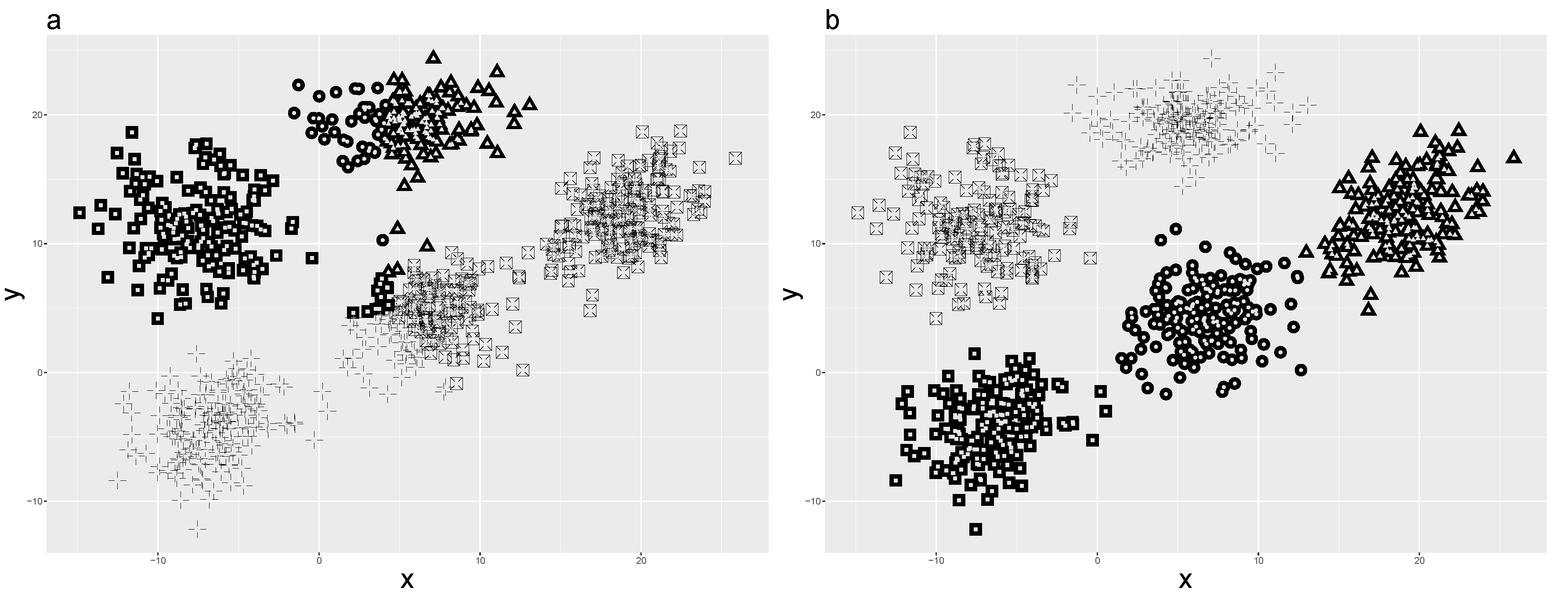
Even though SFKM can adopt any distances, this algorithm was originally simulated in pure numerical and categorical datasets. It performs well in a balanced orientation of a simulated numerical dataset. Unfortunately, when it comes to an unbalanced orientation dataset, the result is poor (Figure 1a). The dataset in Figure 1a has 800 objects with two variables [20]. The objects are assigned into five clusters, and the clusters have a spatially-unbalanced orientation in a two-dimensional space.
Thus, we develop a simple k-medoids (SKM) algorithm, which also applies medoid updating within its clusters in k-medoids setting. The term “simple” is borrowed from the SFKM algorithm for the initial medoids selection. What distinguishes the SFKM and SKM algorithms is that SKM considers the local optima and empty clusters. To minimize the local optima problem, several initializations have been used [21].
The SKM algorithm is as follows:
  • Select a set of initial medoids M k , i.e., selecting k objects from X n , randomly.
    The random initialization is preferred because the random initialization repeated several times is the best approach [21]. However, a restriction is applied to a single point of the M k set. One of the M k sets, which is randomly selected, is replaced by the most centrally-located object. It is argued that an optimal medoid is when k = 1 is the centrally-located object that minimizes the sum distance to the other objects. Then, the most centrally-located object can be selected based on the row/column sum of the distance matrix. It is given as:
    a i = j = 1 n d i j = j = 1 n d j i , i = 1 , 2 , 3 , , n ,
    where a i is the sum distance of the object i to the other objects. If vector a i is ordered, the first M k is selected by the smallest a i , which is the most centrally-located object. Note that one/more medoids from the medoids set M k can be non-unique objects, for example, two medoids have equal values in all their variables.
  • Assign the label/membership of each object x n X n , l ( x n ) , to the closest medoid M k .
    When the medoid set of M k is non-unique objects, an empty cluster can occur because the non-unique medoids and their closest objects will have the same membership label. To avoid an empty cluster, the non-unique medoids are restricted to preserve their label. While the closest objects to the non-unique centroids can be labeled as any cluster membership in the k-means case [18], we regulate that the closest objects to the non-unique medoids are assigned/labeled as only one of the medoids, i.e., a single cluster membership. Hence, this guarantees a faster medoid updating step provided that the non-unique medoid set is not the most centrally-located object.
  • Update the new set of medoids M k , maintaining the clusters label l ( x n ) fixed.
    m p : = a r g m i n p K n : l ( x n ) = m p d ( x n , m p ) , p = 1 , 2 , 3 , , k
    A medoid, m p , is defined as an object that minimizes the sum distance of this object to the other objects within its cluster.
  • Calculate the sum of each cluster sum distance (E), i.e., the sum distance between objects and their medoids.
    E = p = 1 k n : l ( x n ) = m p d ( x n , m p ) .
  • Repeat Steps 2–4 until E is equal to the previous E, or the set of medoids M k does not change, or a pre-determined number of iterations is attained.
  • Repeat Steps 1–5 s times to attain multiple random seeding of the initial medoids.
    Note that the centrally-located object always becomes one of the initial medoids. Among the cluster medoids from the multiple random seeding s, the cluster medoid set that has a minimum value of E is selected as the final cluster medoids.
  • Assign the membership of each object to the final medoids.
The SKM algorithm can be applied in the aforementioned dataset, which yields a better result than the SFKM algorithm (Figure 1b).

2.3. Proposed Distance Method

As a distance-based algorithm, the SKM algorithm input requires a distance function. Compared to distance measures in either numerical or categorical variables, there are limited alternatives for mixed variable distance. Although the most common distance measure for mixed variable data is the Gower distance [9], a generalized distance function (GDF) to increase the variation of the mixed variable choices is developed.
The GDF consists of combinations of weights and distances. It sets particular weights in a linear combination of numerical, binary, and categorical distances. The distance between two objects in the GDF form can be computed by:
d i j = α r = 1 p n δ n ( x i r , x j r ) + β t = 1 p b δ b ( x i t , x j t ) + γ s = 1 p c δ c ( x i s , x j s ) ω ,
where ω is the weight for the whole function, α , β , and γ are the weights for the numerical, binary, and categorical variables, respectively, p n is the number of numerical variables, p b is the number of binary variables, p c is the number of categorical variables, δ n , δ b , and δ c are the numerical, binary, and categorical distances, respectively, and δ n ( x i r , x j r ) is the numerical distance between object i and object j in the variable r.
α , β , and γ are constants implying that each type of all inclusion variables has its own contribution, and each individual variable in the same type equally contributes to the distance computation. When the relative influences of individual variables differ, which can be based on the user domain knowledge or intuition, the constants can be transformed into a vector. This transformation, however, results in a subspace clustering domain [10], which is out of the scope of this article.
By using the GDF, we can reformulate the Gower distance, which is a special case of the GDF. The Gower similarity [9] between object i and object j is normally calculated as:
s i j = l = 1 p ω i j l s i j l l = 1 p ω i j l ,
s i j l = 1 | x i l x j l | R l , o r s i j l { 0 , 1 } ,
where ω i j l is the j th weight of object i in the variable l, x i l is the value of the object i on the l th (numerical) variable, R l is the range of the l th (numerical) variable, and s i j l = 1 if the objects i and j are similar in the l th (binary or categorical) variable and zero otherwise. The Gower distance is then obtained by subtracting one from Equation (2), i.e., d i j = 1 s i j . ω i j l in the Gower distance regulates the contribution of each variable. ω i j l is equal to zero if there is a missing value [22]. When some specific variables are more relevant than others to cluster the objects, ω i j l is unequal [10]. This occurs in the domain of subspace clustering. For a conventional clustering method, on the other hand, equal variable weights ( ω i j l ) for all of the variables are applicable. Thus, the Gower distance for a non-missing value dataset and all variables being equally contributed can be formulated in a GDF form into:
d i j = 1 p n + p b + p c r = 1 p n 1 R r | x i r x j r | + p b t = 1 p b δ b ( x i t , x j t ) + p c s = 1 p c δ c ( x i s , x j s ) ,
where R r is the range of variable r, δ b ( x i t , x j t ) = δ c ( x i s , x j s ) = 0 if object i and object j are similar and one otherwise, i.e., simple matching distance. With equally-contributing variables and without any missing value, Equations (2) and (3) are equal (see Appendix A). Equation (3) implies that the distance for the numerical variable is the Manhattan range weighted, while the distance for the binary and categorical variables is the simple matching.
The other available distances for mixed variable data, which are less popular than the Gower distance, can be transformed into a GDF form in a similar way. They are the Wishart [23], Podani [22], Huang [5], and Harikumar-PV [7] distances. The Wishart and Podani distances have similar properties to the Gower such that the same assumption applies. The Huang and Harikumar-PV distances, on the other hand, do not admit a missing value and have equally-contributing variables by definition. Table 1 shows the GDF formulation of these distances with respect to their distance combinations and weights. Then, other combinations of distances and weights are possible.
3. Demonstration on Artificial and Real Datasets

To apply the proposed k-medoids algorithm (SKM) and distance (GDF), simulated datasets with specified classes (“true clusters”) are generated. The authors of [24] generated artificial data with only numerical variables in arbitrary diameters, shapes, and orientations. In order to obtain a binary/categorical variable for the simulation data, a numerical variable is categorized via a quantile categorization. The categorization of a numerical variable into a binary/categorical variable is obtained by dividing the numerical variable into c classes with the 100 / c % quantile as the cut point. Thus, a binary variable is achieved when the median of the numerical variable is applied as a cutoff point.
The artificial data have a degree of separation parameter [25] that has to be pre-specified. The degree separation values range from −1–1, where one indicates the best-separated clusters. Due to the focus of the study on the different settings of the mixed variable datasets, the degree separation is fixed arbitrarily to 0.2, and all variables are important variables. The mixed variable datasets have four different settings. The variations are in the variables’ proportion, number of clusters, number of variables, and number of objects.
Each setting of the artificial datasets is partitioned by applying the GDFs (Table 1) as the input. Due to the possibility of other combinations of distances and weights in the GDF, two distances derived from the GDF are added, namely the Esimma and Marweco GDFs (Table 2). While the former combines the Euclidean and simple matching distances, the latter sums the Manhattan range weighted distance with the co-occurrence distance. Both GDFs set all of the weights to one.
Then, the k-medoids algorithms, which is compared in this article, are the PAM, the most popular medoid-based algorithm, SFKM, the evaluated algorithm, and SKM ( s = 20 ), the proposed algorithm. To evaluate the algorithms’ performance, the Rand indices are calculated and averaged via a subsetting strategy [26] in 50 replications of the seven GDFs (Table 1 and Table 2). The Rand index is given by:
r i = a + b n C 2 ,
where a and b are the number of pairs of objects in the data. If both object pairs are in the same cluster under the “true cluster” and are also in the same cluster under the particular algorithm, it belongs to a. Meanwhile, b indicates that both object pairs are in a different cluster in both the “true cluster” and particular algorithm.
We also used six real datasets without any missing value from the UCI machine learning repository [27]. These data are the Iris, Wine, Soybean, Vote, Zoo, and Credit approval datasets (Table 3). They were selected due to being commonly used to compare clustering algorithms. Each dataset was analyzed using the proposed SKM algorithm that was applied in the GDFs (Table 1 and Table 2). The performance comparison among GDF variations was based on the clustering accuracy index where perfect clustering had a value of one, and failure of clustering was zero.
To produce the k-medoids algorithms and GDF variations, the analyses were run in the R software [28] applying several packages. The main package was the kmed package [20], which applied the SFKM algorithm and GDFs, while the PAM algorithm was applied in the cluster package [29]. The SKM algorithm, on the other hand, was written in an R code and is available in the Supplementary Material. The clusterGeneration [30] was also applied to generate the artificial data; the flexclust package [31] had the Rand index function; and the clue package [32] were able to calculate the clustering accuracy. Last, the ggplot2 [33] and gridExtra [34] packages helped the visualization results. With an Intel i3 4GB RAM, all codes required about 90 min to produce the results.

3.1. Data Simulation

3.1.1. Different Variable Proportions

The artificial data had four cases with different variable proportions. The variations of the variable proportions included mixed variable datasets with numerical, binary, and categorical variable domination. In any variable domination, the SFKM had the lowest Rand index and was significantly different from PAM and SKM (Table 4). When the variable domination was categorical variables with the number of variables equal to three in the Huang GDF, the Rand index of the SFKM algorithm (0.70) was the highest compared to the other two algorithms. However, in this variable domination, high Rand indices were achieved in the Podani GDF (0.78) in both the PAM and SKM algorithms where the SFKM algorithm had only 0.71 of the Rand index.

3.1.2. Different Number of Clusters

The artificial data generated four different numbers of clusters. The numbers of clusters were 3, 4, 8, and 10. In any number of clusters, the SFKM algorithm always gave the smallest Rand index and was different from the other two algorithms (Table 5). When the number of clusters was small, i.e., k = 3 , and the GDF was Marweco, the Rand index of the SFKM was the highest (0.84) compared to other GDFs. Both PAM and SKM, however, had a higher Rand index (0.88), and it was statistically different from that of the SFKM. Meanwhile, if the number of clusters was large ( k = 10 ), the highest Rand index (0.91) of both the PAM and SKM was the Huang GDF. Although the Rand index of the SFKM was slightly lower than the other two, i.e., 0.90, it was statistically different. The result showed that SFKM was the most underperforming algorithm.

3.1.3. Different Numbers of Variables

The artificial data simulated a different number of mixed variables. The numbers of the mixed variables were 6, 8, 10, and 14. In any number of mixed variables, the SFKM algorithm showed underperforming results (Table 6). When the number of mixed variables was six and the GDFs were Huang and Harikumar, the Rand index of the SFKM algorithm (0.70) was the highest compared to the other two algorithms. Nevertheless, high Rand indices were attained by the Gower GDF (0.85) in both the PAM and SKM algorithms, where the SFKM algorithm had only 0.79 of the Rand index.

3.1.4. Different Numbers of Objects

The artificial data had variations in the number of objects. The datasets had 100, 500, 1000, and 2000 objects. Overall, both PAM and SKM had better results than SFKM (Table 7). They shared similar high Rand indices (≥0.95) when the number of objects was 2000 in the Huang, Harikumar-PV, and Esimma GDFs. However, although SFKM had a high index in the Harikumar-PV GDF, it was significantly different from both the PAM and SKM algorithms.
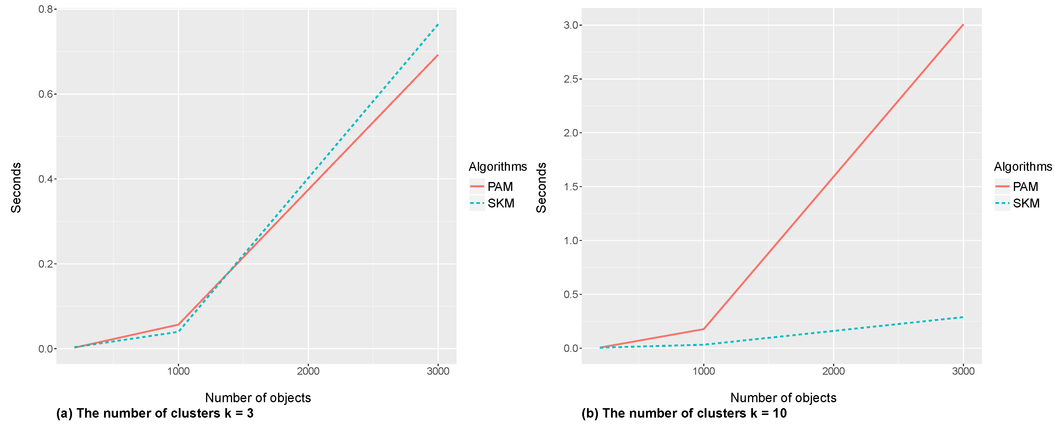
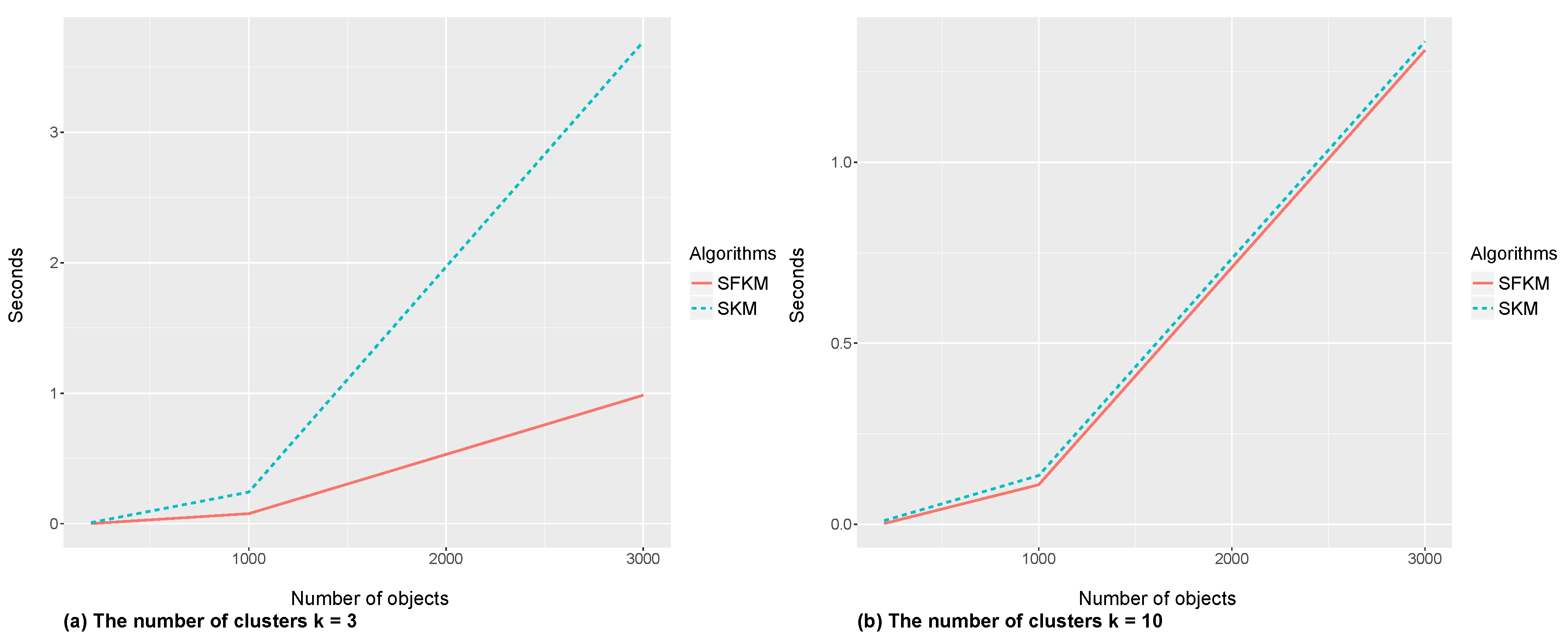
Table 4, Table 5, Table 6 and Table 7 show that the proposed k-medoids (SKM) had better performance than the evaluated algorithm (SFKM). In all settings, the Rand indices between the “true cluster” and SKM algorithm were higher than those between the “true cluster” and SFKM algorithm. On the other hand, from the running time perspective, theoretically, the SKM algorithm required more time than the SFKM algorithm due to repetition sets vs. a single set of initial medoids. By applying s times the multiple random seeding, the SKM finished a partitioning algorithm in a maximum of s multiplied by the required time of the SFKM. A simulation of k = 3 and k = 10 with s = 20 in the SKM, however, had an insignificant gap from the SFKM when the number of clusters was large (Figure 2).
Although the SFKM algorithm, which applied a specific formula for the initial medoid selection, gained speed, it performed badly with respect to the external validation, i.e., Rand index. With the current advancement in computation, in addition, the speed of the SKM algorithm could be increased. Due to the independent random seedings as many as s times, parallel computation was feasible to gain speed in the SKM. Hence, the SKM could be as fast as the SFKM when the number of cores was s. Although it was suggested to repeat the algorithm as many times as possible to avoid the local optima problem [17], with 20 seedings, the SKM algorithm yielded a similar result to the popular PAM algorithm. Then, the SKM and PAM algorithms were compared with respect to their efficiency.
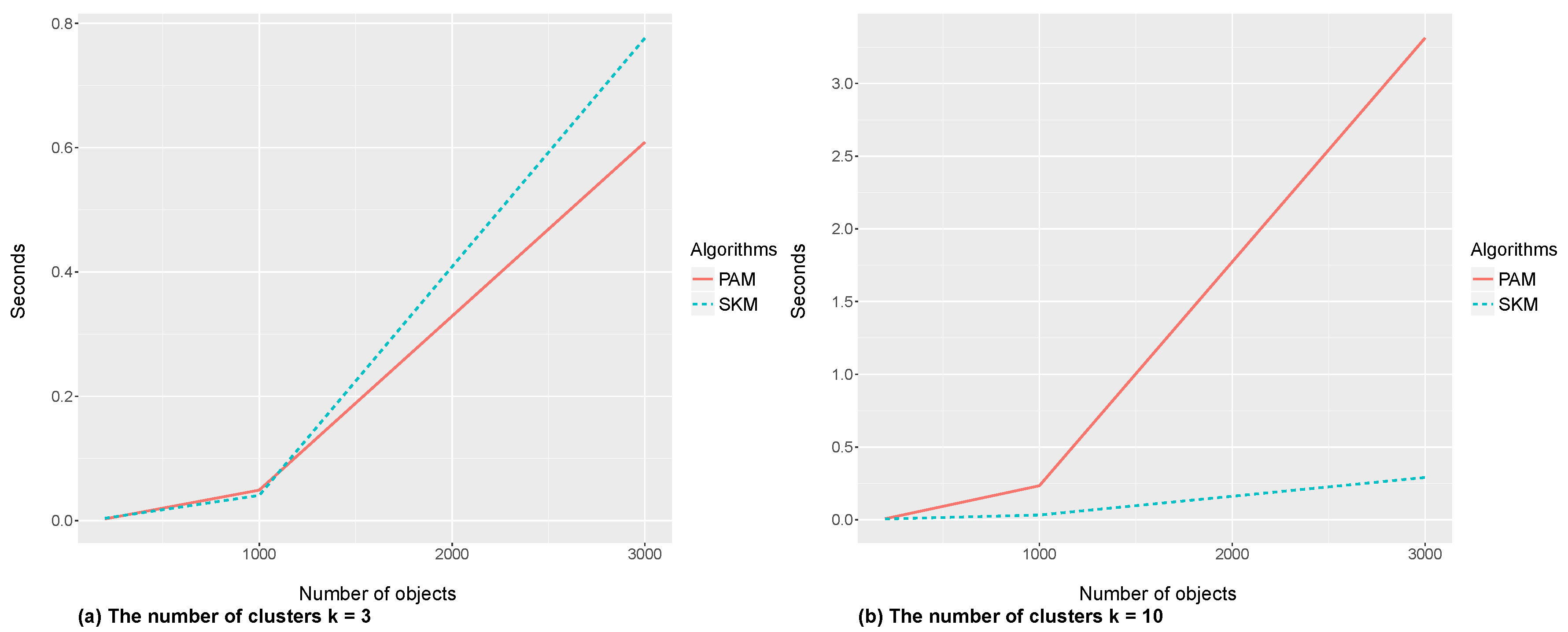
The comparison took two different numbers of clusters ( k = 3 , 10 ) in small and large numbers of objects ( n = 200 , 1000 , 3000 ). Each evaluation was averaged over 50 replications with seconds as the evaluation unit. The comparison also applied two different random number generators ( s e t . s e e d ). Figure 3 and Figure 4 show that PAM had a faster run time than SKM when the number of clusters was small ( k = 3 ) and the number of objects was large ( n > 1000 ). With large k and n ( k = 10 , n > 1000 ), on the other hand, SKM required less time compared to PAM. Thus, SKM and PAM were on par for small n and k.

3.2. Real Datasets

3.2.1. Iris Data

The Iris dataset has no binary and categorical variables, albeit that it has only four numerical variables with 150 objects assigned to an equal size of three classes. We applied the seven GDFs and one additional Canberra GDF. The maximum clustering accuracy was 95.3% for the Canberra GDF. Comparing to the k-means [6] and k-prototype [13] for the mixed and categorical variable algorithms, the clustering accuracy of the SKM algorithm, which applied the Canberra GDF, was the highest (Table 8).

3.2.2. Wine Data

The wine dataset has 13 numerical variables with 178 objects assigned to three classes. The seven GDFs and Canberra GDF were applied. The highest accuracy index 92.7% was achieved when the Podani GDF was applied. If SFKM, k-harmonic means, and ranked k-medoids were applied to the wine data, the clustering accuracy indices gained only 70.4%, 68.5%, and 70.3%, respectively [19].

3.2.3. Soybean Data

The Soybean dataset only consists of categorical variables with 35 categorical variables and 47 objects attributed to four classes. Due to the absence of the numerical and binary variables, the seven GDFs were reduced to five GDFs. The two GDFs were the Esimma and Marweco GDFs that were equal to the Gower and Harikumar-PV, respectively. In the Soybean data, the Gower/ Esimma, Wishart, Harikumar-PV/ Marweco gained the maximum clustering accuracy, i.e., 100%. They out-performed both the k-prototype [13] and SFKM [16] algorithms.

3.2.4. Vote Data

The Vote dataset only consists of categorical variables with 16 categorical variables and 435 objects attributed to two classes. Harikumar-PV/ Marweco achieved 87.8% as the highest clustering accuracy. Compared to the k-prototype, hierarchical, and k-means for the mixed and categorical variables algorithms, they achieved 83.7%, 85.5%, and 86.7% clustering accuracy, respectively [6].

3.2.5. Zoo Data

The Zoo data have 101 objects assigned to seven classes. These data are mixed variables with one numerical and 15 binary variables. The seven GDFs were applied. The maximum clustering accuracy index was 82.2% for the Marweco GDF. Although the rank k-medoids [19] offered local optima way out through asymmetric distance, the clustering accuracy of the Zoo data was only 78.7% (Table 8).

3.2.6. Credit Approval Data

The Credit approval data have 653 objects (without NA) assigned to two classes. This dataset is mixed variables with six numerical and nine categorical variables. The seven GDFs were applied in the credit approval data. The maximum clustering accuracy index was 82.7% for the Marweco GDF. For this dataset, the author of [13] listed the clustering accuracy of other algorithms such as the k-prototype (56.2%), similarity-based agglomerative clustering (SBAC) (55.5%), KL-FCM-GM (Kullback–Leibler fuzzy c-means Gauss multinomial) (57.4%), and k-prototype for the mixed and categorical variables (77.9%) [13].
Table 8 shows that the SKM had better performances in all real datasets. Notice that the other algorithms in Table 8 may apply a different distance method. The SKM algorithm in the Iris dataset, for instance, applied the Canberra GDF that was compared to the k-means and k-prototype with the Euclidean distance. Although it appeared to be an unfair comparison due to the different GDF (distance) selections, our comparison emphasized the GDF’s advantage in its combinations of the distances and weights.
The flexible combinations of the distances are an important feature of the GDF. While there are many alternatives for numerical, binary, and categorical distances, the mixed variable distances have few options. The more variations in the mixed variable distance are of the utmost importance due to the distance function exerting a major effect on a partitioning algorithm’s result [35], i.e., different distances producing different optima. Hence, with the GDF’s flexibility, various distance combinations and weights can be simply applied. The Esimma and Marweco GDFs were the two GDF examples that were applied showing the GDF benefit.
Due to the linear combination of the numerical, binary, and categorical variables independently, another advantage of the GDF is that each distance class can be also canceled out when a class variable is excluded in a dataset. If a dataset only consists of numerical variables, for instance, the distance involved is only a numerical distance by eliminating the binary and categorical distances. The Canberra GDF in the Iris data, for example, emerged because the binary and categorical distances were omitted.
An adjustable weight to set a different contribution of an individual variable is the last advantage of the GDF. While the GDF had a scalar (constant) weight for α , β , and γ , it can be replaced by a vector of weights. The vector of weights implies that each variable has its own contribution to the distance computation, i.e., the variables do not equally contribute. Unequal contributions of the variables have been applied iteratively in the subspace clustering of the k-means algorithm by updated weights [36]. If a vector of weights is applied in the GDF, on the other hand, the contribution of the variables is calculated only once compared to as many as the iterations in the updated weights. Thus, the vector of weights in the GDF is preferred in a medoid-based algorithm setting than the updated weights.

4. Conclusions

A simple k-medoids (SKM) algorithm was proposed in this paper. To supply the distance as an input in this algorithm, a generalized distance function (GDF) was also developed. This function was adjustable to any type of data, and when the data were mixed variables, flexible combinations of the distances and weights were gained. Compared to the simple and fast k-medoids (SFKM) [16], which had a similar way in the within-cluster medoid updating, the SKM surpassed any mixed variable data case. The SKM performance was also similar to the PAM. With the s parameter as the number of initializations, a number of s equal to 20 was sufficient to produce a similar result to the PAM. When the numbers of clusters and objects were few, the run times of the SKM and PAM were similar. However, the SKM required less time for a large number of clusters and objects. The partitioning results of the six real datasets showed that the SKM had a better cluster accuracy index compared to other partitioning algorithms. Moreover, there is an R package, which is available from CRAN, called kmed, that implements both SFKM and GDF.

Supplementary Materials

The following are available online at: https://www.mdpi.com/1999-4893/12/9/177/s1. All Supplementary Materials are also available from the OSF (Open Science Framework) account of the corresponding author (http://www.doi.org/10.17605/OSF.IO/CNQTA).

Author Contributions

Conceptualization, W.B. and F.L.; methodology, W.B. and F.L.; programming and coding, W.B.; visualization, W.B.; writing, original draft preparation, W.B.; writing, review and editing, W.B. and F.L.; supervision, F.L.

Funding

This research was funded by Ditjen Sumberdaya IPTEK DIKTI (No. 138.44/E4.4/2015) and OeAD (ICM-2018-11915). The APC was funded by Institute of Statistics, University of Natural Resources and Life Sciences.

Acknowledgments

The authors would like to thank Ditjen Sumberdaya, the Ministry of Research, Technology, and Higher Education of Indonesia, Kemenristekdikti, and OeAD, Österreichischer Austauschdienst, for the continuous support via the Indonesia Austria Scholarship Program (IASP).

Conflicts of Interest

The authors declare no conflict of interest.

Abbreviations

The following abbreviations are used in this manuscript:
GDFGeneralized distance function
KMK-medoids
PAMPartitioning around medoids
SFKMSimple and fast k-medoids
SKMSimple k-medoids

Appendix A

The Gower distance of objects i and j is defined as d i j = 1 s i j . Assuming no missing value and equally-contributing variables, i.e., ω i j l = 1 , d i j with a single variable of the numerical, binary, and categorical variables becomes:
d i j = 1 s i j = 1 s i j n u m e r i c a l + s i j b i n a r y + s i j c a t e g o r i c a l 1 + 1 + 1 = 1 s i j n u m e r i c a l + s i j b i n a r y + s i j c a t e g o r i c a l 3 = 3 ( s i j n u m e r i c a l + s i j b i n a r y + s i j c a t e g o r i c a l ) 3 = ( 1 s i j n u m e r i c a l ) + ( 1 s i j b i n a r y ) + ( 1 s i j c a t e g o r i c a l ) 3 = ( 1 ( 1 | x i x j | R ) ) + d i j b i n a r y + d i j c a t e g o r i c a l 3 = | x i x j | R + d i j b i n a r y + d i j c a t e g o r i c a l 3 .
When the numbers of numerical, binary, and categorical variables are p n , p b , and p c , respectively, the Gower distance of objects i and j is:
d i j = r = 1 p n | x i r x j r | R r + t = 1 p b d i j b i n a r y + s = 1 p c d i j c a t e g o r i c a l p n + p b + p c = r = 1 p n | x i r x j r | R r + p b t = 1 p b d i j b i n a r y p b + p c s = 1 p c d i j c a t e g o r i c a l p c p n + p b + p c = 1 p n + p b + p c r = 1 p n 1 R r | x i r x j r | + p b t = 1 p b δ b ( x i t , x j t ) + p c s = 1 p c δ c ( x i s , x j s ) ,
where both the δ b ( x i t , x j t ) and δ c ( x i s , x j s ) are simple matching distances.

References

  1. Gan, G.; Ma, C.; Wu, J. Data Clustering, Theory, Algorithm, and Application; The American Statistical Association; The Society for Industrial and Applied Mathematics: Philadelphia, PA, USA, 2007. [Google Scholar]
  2. Kaufman, L.; Rousseeuw, P.J. Finding Groups in Data; John Wiley and Sons Inc.: New York, NY, USA, 1990. [Google Scholar]
  3. Hartigan, J.A.; Wong, M.A. A K-Means Clustering Algorithm. J. R. Stat. Soc. 1979, 28, 100–108. [Google Scholar]
  4. Wu, X.; Kumar, V.; Quinlan, J.R.; Ghosh, J.; Yang, Q.; Motoda, H.; McLachlan, G.J.; Ng, A.; Liu, B.; Yu, P.S.; et al. Top 10 algorithms in data mining. Knowl. Inf. Syst. 2008, 14, 1–37. [Google Scholar] [CrossRef]
  5. Huang, Z. Clustering large datasets with mixed numeric and categorical values. In Proceedings of the First Pacific-Asia Conference on Knowledge Discovery and Data Mining; Springer: Berlin, Germany, 1997; pp. 21–34. [Google Scholar]
  6. Ahmad, A.; Dey, L. A K-mean clustering algorithm for mixed numeric and categorical data. Data Knowl. Eng. 2007, 63, 503–527. [Google Scholar] [CrossRef]
  7. Harikumar, S.; Surya, P.V. K-Medoid Clustering for Heterogeneous DataSets. Procedia Comput. Sci. 2015, 70, 226–237. [Google Scholar] [CrossRef] [Green Version]
  8. McCane, B.; Albert, M. Distance functions for categorical and mixed variables. Pattern Recognit. Lett. 2008, 29, 986–993. [Google Scholar] [CrossRef] [Green Version]
  9. Gower, J.C. A General Coefficient of Similarity and Some of Its Properties. Biometrics 1971, 27, 857–871. [Google Scholar] [CrossRef]
  10. Friedman, J.H.; Meulman, J.J. Clustering objects on subsets of attributes (with discussion). J. R. Stat. Soc. Ser. B 2004, 66, 815–849. [Google Scholar] [CrossRef]
  11. Yin, J.; Tan, Z. Clustering Mixed Type Attributes in Large Dataset. In ISPA 2005: Parallel and Distributed Processing Application; Pan, Y., Chen, D., Guo, M., Cao, J., Dongarra, J., Eds.; Lecture Notes in Computer Science Volumn 3758; Springer: Berlin/Heidelberg, Germany, 2005; pp. 655–661. [Google Scholar]
  12. Bushel, P.R.; Wolfinger, R.D.; Gibson, G. Simultaneous clustering of gene expression data with clinical chemistry and pathological evaluations reveals phenotypic prototypes. BMC Syst. Biol. 2007, 1, 1–20. [Google Scholar] [CrossRef]
  13. Ji, J.; Bai, T.; Zhou, C.; Ma, C.; Wang, Z. An improved k-prototypes clustering algorithm for mixed numeric and categorical data. Neurocomputing 2013, 120, 590–596. [Google Scholar] [CrossRef]
  14. Liu, S.H.; Shen, L.Z.; Huang, D.C. A three-stage framework for clustering mixed data. WSEAS Trans. Syst. 2016, 15, 1–10. [Google Scholar]
  15. Reynolds, A.P.; Richards, G.; De La Iglesia, B.; Rayward-Smith, V.J. Clustering Rules: A Comparison of Partitioning and Hierarchical Clustering Algorithms. J. Math. Model. Algorithms 2006, 5, 475–504. [Google Scholar] [CrossRef]
  16. Park, H.; Jun, C. A simple and fast algorithm for K-medoids clustering. Expert Syst. Appl. 2009, 36, 3336–3341. [Google Scholar] [CrossRef]
  17. Steinley, D. Local Optima in K-Means Clustering: What You Don’t Know May Hurt You. Psychol. Methods 2003, 8, 294–304. [Google Scholar] [CrossRef]
  18. Pakhira, M.K. A Modified k-means Algorithm to Avoid Empty Clusters. Int. J. Recent Trends Eng. 2009, 1, 221–226. [Google Scholar]
  19. Zadegan, S.M.R.; Mirzaie, M.; Sadoughi, F. Ranked k-medoids: A fast and accurate rank-based partitioning algorithm for clustering large datasets. Knowl.-Based Syst. 2016, 39, 133–143. [Google Scholar] [CrossRef]
  20. Budiaji, W.; kmed: Distance-Based K-Medoids. R Package Version 0.3.0. 2019. Available online: http://CRAN.R-project.org/package=kmed (accessed on 15 June 2019).
  21. Steinley, D.; Brusco, M. Initializing K-means Batch Clustering: A Critical Evaluation of Several Techniques. J. Classif. 2007, 24, 99–121. [Google Scholar] [CrossRef]
  22. Podani, J. Introduction to Exploration of Multivariate Biological Data; Backhuys Publishers: Leiden, The Netherlands, 2000. [Google Scholar]
  23. Wishart, D. K-Means Clustering with Outlier Detection, Mixed Variables and Missing Values. In Exploratory Data Analysis in Empirical Research, Proceedings of the 25th Annual Conference of the Gesellschaft für Klassifikation e.V., University of Munich, 14–16 March 2001; Springer: Berlin/Heidelberg, Germany, 2003; pp. 216–226. [Google Scholar]
  24. Qiu, W.; Joe, H. Generation of Random Clusters with Specified Degree of Separation. J. Classif. 2006, 23, 315–334. [Google Scholar] [CrossRef]
  25. Qiu, W.; Joe, H. Separation Index and Partial Membership for Clustering. Comput. Stat. Data Anal. 2006, 50, 585–603. [Google Scholar] [CrossRef]
  26. Hennig, C. Cluster-wise assessment of cluster stability. Comput. Stat. Data Anal. 2007, 52, 258–271. [Google Scholar] [CrossRef] [Green Version]
  27. Lichman, M. UCI Machine Learning Repository; University of California: Irvine, CA, USA, 2013; Available online: http://archive.ics.uci.edu/ml (accessed on 17 July 2018).
  28. R Core Team. R: A Language and Environment for Statistical Computing; R Foundation for Statistical Computing: Vienna, Austria, 2015; Available online: https://www.R-project.org/ (accessed on 2 January 2017).
  29. Maechler, M.; Rousseeuw, P.; Struyf, A.; Hubert, M.; Hornik, K.; cluster: Cluster Analysis Basics and Extensions. R Package Version 2.0.6—For New Features, See the ‘Changelog’ File (in the Package Source). 2017. Available online: http://CRAN.R-project.org/package=cluster (accessed on 10 September 2018).
  30. Qiu, W.; Joe, H. clusterGeneration: Random Cluster Generation (with Specified Degree of Separation). R Package Version 1.3.4. 2015. Available online: http://CRAN.R-project.org/package=clusterGeneration (accessed on 23 August 2018).
  31. Leisch, L.; Dimitriadou, D.; Gruen, B.; flexclust: Flexible Cluster Algorithms. R Package Version 1.4-0. 2018. Available online: http://CRAN.R-project.org/package=flexclust (accessed on 15 January 2019).
  32. Hornik, K.; Böhm, W.; clue: Cluster Ensembles. R Package Version 0.3-57. 2019. Available online: http://CRAN.R-project.org/package=clue (accessed on 7 May 2019).
  33. Wickham, H. ggplot2: Elegant Graphics for Data Analysis; Springer: New York, NY, USA, 2016. [Google Scholar]
  34. Auguie, B.; Antonov, A.; gridExtra: Miscellaneous Functions for “Grid” Graphics. R Package Version 2.3. 2017. Available online: http://CRAN.R-project.org/package=gridExtra (accessed on 1 May 2018).
  35. Leisch, F. A toolbox for K-centroids cluster analysis. Comput. Stat. Data Anal. 2006, 51, 526–544. [Google Scholar] [CrossRef]
  36. Ahmad, A.; Dey, L. K-means type clustering algorithm for subspace clustering of mixed numeric and categorical datasets. Pattern Recognit. Lett. 2011, 32, 1062–1069. [Google Scholar] [CrossRef]
Figure 1. The simple and fast k-medoids (SFKM) (a) and simple k-medoids (SKM) (b) partitioning results.
Algorithms 12 00177 g001
Figure 2. Benchmarking of the SKM and SFKM for k = 3 (a) and k = 10 (b).
Algorithms 12 00177 g002
Figure 3. Benchmarking of PAM and SKM for k = 3 (a) and k = 10 (b) with s e t . s e e d ( 2018 ) .
Algorithms 12 00177 g003
Figure 4. Benchmarking of PAM and SKM for k = 3 (a) and k = 10 (b) with s e t . s e e d ( 2019 ) .
Algorithms 12 00177 g004
Table 1. Mixed variable distances in the GDF formulation.
GDF ω α β γ δ n ( x ir , x jr ) δ b ( x it , x jt ) δ c ( x is , x js )
Gower1 1 p n + p b + p c p b p n + p b + p c p c p n + p b + p c M rwSMSM
Wishart 1 2 1 p n + p b + p c p b p n + p b + p c p c p n + p b + p c SE vwSMSM
Podani 1 2 1 p b p c SE r 2 wSMSM
Huang11 s n ¯ s n ¯ SEHH
Harikumar-PV1111MHCoC
p n = number of numerical variables, p b = number of binary variables, p c = number of categorical variables, s n ¯ = mean of the standard deviation of numerical variables, H = Hamming, M = Manhattan, SE = squared Euclidean, SM = simple matching, CoC = co-occurrence, rw = range weighted, r 2 w = squared range weighted, vw = variance weighted.
Table 2. Two examples of the mixed variable distances derived from the generalized distance function (GDF).
GDF ω α β γ δ n ( x ir , x jr ) δ b ( x it , x jt ) δ c ( x is , x js )
Esimma1111ESMSM
Marweco1111M rwCoCCoC
E = Euclidean, CoC = co-occurrence, SM = simple matching, M = Manhattan, rw = range weighted.
Table 3. Details of the real datasets.
Data Setn p n p b p c k
Iris1504003
Wine17813003
Soybean4700354
Vote43500162
Zoo10111507
Credit approval6536092
n = number of objects, p n , p b , p c = number of numerical, binary, and categorical variables, respectively, k = number of true clusters.
Table 4. Rand indices of the different proportions of variables.
DominationAlgorithmGowerWishartPodaniHuangHarikumarEsimmaMarweco
NumericalPAM0.740.820.730.840.830.850.82
SFKM0.72 a 0.73 a 0.71 a 0.74 a 0.71 a 0.76 a 0.71 a
SKM0.740.800.730.840.830.850.82
BinaryPAM0.780.780.770.770.760.730.74
SFKM0.74 a 0.73 a 0.73 a 0.74 a 0.72 a 0.73 c 0.73 c
SKM0.780.770.780.770.750.740.75
CategoricalPAM0.780.760.780.690.680.670.74
c = 3 SFKM0.71 a 0.72 a 0.71 a 0.70 a 0.680.670.70 a
SKM0.770.750.780.690.680.670.74
CategoricalPAM0.770.820.770.790.780.760.77
c = 5 SFKM0.71 a 0.75 a 0.71 a 0.790.790.760.69 a
SKM0.760.810.770.790.780.760.77
Significantly different ( α = 0.05 ) from: a PAM and SKM, c SKM.
Table 5. Rand indices of the different numbers of clusters.
kAlgorithmGowerWishartPodaniHuangHarikumarEsimmaMarweco
3PAM0.830.870.810.810.830.840.88
SFKM0.79 a 0.83 a 0.76 a 0.79 a 0.810.81 a 0.84 a
SKM0.830.870.810.790.810.840.88
4PAM0.760.880.740.890.900.900.84
SFKM0.72 a 0.84 a 0.730.86 a 0.86 a 0.88 a 0.80 a
SKM0.770.880.740.890.900.900.84
8PAM0.820.910.810.910.900.910.88
SFKM0.80 a 0.87 a 0.80 a 0.89 a 0.87 a 0.89 a 0.84 a
SKM0.810.900.810.910.900.900.87
10PAM0.860.920.850.910.910.910.89
SFKM0.84 a 0.88 a 0.85 a 0.90 a 0.88 a 0.90 a 0.85 a
SKM0.850.900.850.910.900.910.87
Significantly different ( α = 0.05 ) from: a PAM and SKM.
Table 6. Rand indices of the different numbers of variables.
pAlgorithmGowerWishartPodaniHuangHarikumarEsimmaMarweco
6PAM0.850.770.830.690.690.690.79
SFKM0.79 a 0.75 b 0.81 a 0.70 b 0.70 c 0.700.77 c
SKM0.840.760.840.690.690.690.79
8PAM0.800.930.790.900.900.920.86
SFKM0.74 a 0.86 a 0.75 a 0.88 a 0.84 a 0.88 a 0.79 a
SKM0.800.930.790.910.900.920.86
10PAM0.740.770.730.760.760.760.76
SFKM0.71 a 0.73 a 0.71 a 0.74 a 0.73 a 0.74 a 0.70 a
SKM0.740.760.730.750.760.760.75
14PAM0.690.850.680.950.950.950.89
SFKM0.66 a 0.78 a 0.66 a 0.85 a 0.81 a 0.86 a 0.79 a
SKM0.690.850.670.950.950.950.89
Significantly different ( α = 0.05 ) from: a PAM and SKM, b PAM, c SKM.
Table 7. Rand indices of the different numbers of objects.
nAlgorithmGowerWishartPodaniHuangHarikumarEsimmaMarweco
100PAM0.750.870.730.940.930.950.91
SFKM0.72 b 0.84 a 0.730.89 a 0.88 a 0.89 a 0.85 a
SKM0.740.880.730.940.930.940.91
500PAM0.760.930.750.910.900.920.92
SFKM0.74 a 0.88 a 0.740.88 a 0.87 a 0.90 a 0.89 a
SKM0.760.930.750.910.890.920.92
1000PAM0.750.880.750.860.890.890.85
SFKM0.73 a 0.81 a 0.740.860.86 a 0.87 a 0.84
SKM0.760.880.740.860.890.890.85
2000PAM0.770.960.770.980.980.980.95
SFKM0.76 a 0.91 a 0.76 a 0.970.95 a 0.970.92 a
SKM0.780.960.770.980.980.980.95
Significantly different ( α = 0.05 ) from: a PAM and SKM, b PAM, c SKM.
Table 8. Clustering accuracy (in percent) of the real datasets.
DatasetTypeSKMOther Algorithms
IrisNumerical95.394.7 [6] a , 82.2 [13] b
WineNumerical92.770.3 [19] c
SoybeanCategorical10091.0 [13] b , 81.0 [16] d
VoteCategorical87.886.7 [6] a
ZooMixed82.278.7 [19] c
Credit approvalMixed82.777.9 [13] b
a k-means for mixed and categorical variables, b k-prototype for mixed and categorical variables, c rank k-medoids, d SFKM.