Abstract
The RTD-A (robust, tracking, disturbance rejection and aggressiveness) controller is a novel control scheme that substitutes the classical proportional integral derivative (PID) controller. This novel controller’s performance depends on the four controller tuning parameters (θR, θT, θD and θA). The tuning of RTD-A controller is more transparent than classic PID controllers. The RTD-A tuning parameters values lies between ZERO and ONE. Availability of a tool to design optimal parameters for this controller and evaluating the performance on a given system is necessary for the researchers. In this paper, the new simulation tool is presented to deal with the RTD-A control scheme. There are four graphical user interface tools included in the proposed tool and working of each tool is explained in detail. To demonstrate the proposed tool, two examples, which involve a liquid level control application and an air pressure control application, are presented in this work. The performance of the RTD-A controller is compared with PID controller. RTD-A controllers are tuned using optimization algorithms and their performances are observed and analyzed in both cases under deterministic and uncertain conditions.
1. Introduction
The proportional integral and derivative (PID) controllers are mostly used to control the critical processes in all over the industries. Most of the industrial closed loop control schemes use the PID controller [1]. Implementing a PID controller is an easy task by considering its simple structure [2]. The process becomes complex by adding a disturbance signal with uncertainty process parameters. The PID controller depends on technology, which is inefficient to fulfill the need of the 21st century. In general, classical control schemes have been positively used only on well-defined plant models [3]. The PID controller has three tuning parameters, which are the proportional gain (KP), integral gain (KI) and derivative gain (KD) [4,5]. The PID controller parameters are difficult to tune in achieving more robust performance with the existence of process uncertainties [6]. Even after choosing the tuning values user will be facing difficulties in achieving the disturbance rejection and set point tracking simultaneously within the restricted time. Most of the industrial processes need a controller with the combo of set point tracking and disturbance rejection ability, which is challenging with the classic PID controller. One may get some unsatisfactory results using tuning rules such as Ziegler–Nichols (ZN) and Cohen–Coon (CC) [7]. It may be debated that contemporary optimization techniques have made the classical tuning methods needless. These techniques mandate a reliable plant model, which is to be controlled effectively [8]. The user can solve the problem of optimization by considering some advanced version of control scheme such as the model predictive controller (MPC). MPC can be effective in the typical industry situations, but still, they have certain limitations, which are generally not mentioned in advance process control applications. The limitations are difficulty in industry operations, high maintenance cost and less flexibility towards industrial functioning. All the mentioned limits may lead to insubstantial controllers that are not cost-effective. There are many discrepancies while calculating the tuning parameters [9]. The Smith predictor algorithm can be implemented across the controller transfer function for reducing the effect of dead time on the process output. Internal model control (IMC) has the advantage of robust tuning rules, but it has the disadvantage of a large process time constant. In the IMC scheme the user needs to choose integral time equal to the process time constant [10]. Therefore, it is inevitable to design a novel alternate control scheme that has all the combined advantages of PID and MPC.
In 2005, Ogunnaike and Kapil Mukati had introduced a new control algorithm RTD-A, which is more efficient than PID for chemical and other industrial processes [11]. The RTD-A controller is introduced to rectify all the disadvantages of classical controllers such as PID, IMC and MPC. This controller tuning is based on the characteristics such as robustness, tracking, disturbance rejection and aggressiveness of the controller, which is prefixed as RTD-A controller. The RTD-A controller can be implemented only in discrete time. The performance of the controller is greatly influenced by the sampling time and therefore a careful selection of sampling time is inevitable. The clear relationship between the RTD-A controller tuning parameters and characteristics is very well explained and also robust stability of the proposed regulatory controller investigated by Ogunnaike and Kapil Mukati [12,13]. In 2011 Vinay Kariwala introduced the block diagram representation of RTD-A controller implementation and an alternate tuning rule. The rules are focused on optimizing the results, but the Kariwala algorithm was working better than the Ogunnaike rules [14]. In the past, there are tools such as the fractional order modeling and control (FOMCON), Jonathan model predictive controller (jMPC) and N-integer. They could be used for real-time applications. FOMCON is the tool made for the researcher to understand the concept of the fractional order controller technique. The jMPC tool is made for dealing with the model predictive controller in real-time implementation and the N-integer tool is the basic version of the fractional order control [15,16,17]. The proposed tool is inspired by an educational tool developed by Daniel Carmona Morales for optimal PID tuning using evolutionary strategies in a multi-input multi-output process control application [18]. It is notable that several simulation tools are already available to design various controllers using classical tuning approaches. The researchers can easily understand the new control schemes through hands-on practices using simulation tools [19]. From an educational point of view, the proposed tool will be useful to understand the RTD-A controller concept and characteristics very effectually.
The main contribution of this paper is to introduce a new graphical user interface (GUI) simulation tool for RTD-A controller based on MATLAB, which contains two tuning rules on a single platform in order to control the chosen process as well as analyze the performance of the same. There are four graphical user interface (GUI) tools in the proposed tool. The first tool can reduce the higher order transfer function into first order process with dead time (FOPDT) because the plant model is used to determine the various controller parameters, which will minimize the different performance measures. The second tool deals with basic facility for tuning the RTD-A controller and plotting the closed loop step response, whereas the third tool allows the user to manually adjust and examine the effect of each RTD-A tuning parameters on the process output through GUI [20]. The fourth tool has the facility to find the optimal tuning parameter values using five optimization algorithms such as galactic swarm optimization (GSO), genetic algorithm (GA), particle swarm optimization (PSO), firefly optimization (FFA) and grey wolf algorithm (GWA), which are arbitrarily chosen for the tool design. There are bio-inspired optimization algorithms that can also be used to tune the classical and RTD-A controller parameters [21]. Yugi Fan proposed beetle antennae search algorithm to tune PID controller for controlling the position of electro-hydraulic servo system [22]. The hybrid of the PSO and GA algorithm is used to self-tune PID for the hydraulic cylinder pressure control [23]. Bilal introduced an improved cuckoo search (CS) algorithm called island based CS. It has two improvements over the basic CS algorithm. It can effectively control the diversity of its population and enhance the exploration of the algorithm [24]. In 2017, a new set of evolutionary algorithm called the estimation of distribution algorithms were introduced by Antonio. It is used to find an optimal solution for complex problems [25]. An ideal gas optimization algorithm based on the first law of thermodynamics and kinetic energy is proposed by Masumeh. The performance of the proposed algorithm compared with the PSO and GA [26]. In 2019, Radu-Emil Precup discussed optimal tuning of the proportional integral fuzzy controller for a servo position control system using nature inspired optimization algorithms. The PSO, GSA, GWO and charged systems search optimization algorithms were used in this application. A hybrid of algorithms was also proposed and compared with the adaptive fuzzy controlled servo system performance [27].
The outline of the paper is organized in the following sections; the concept of the RTD-A control scheme and stability analysis is introduced in Section 2. The effect of RTD-A parameter on the process output is discussed in Section 3. In Section 4, Implementation of RTD-A algorithm with the tool is explained. Section 5 gives the simulation results of the controller. The conclusion and future scope of the work is presented in Section 6.
2. RTD-A Control Scheme
The basic control scheme of the RTD-A controller is discussed in this section. The general closed loop block diagram with the RTD-A controller is shown in Figure 1. There is adequate research going on to find the appropriate alternative algorithm for the PID controller. This alternative RTD-A controller is also known as the regulatory controller [11]. This controller is basically an implementation of an algorithm designed to have the robustness characteristics, tracking ability, disturbance rejection capability and aggressive property. Initially, Kapil Mukati and Ogunnaike have developed a tuning rule that deals with the parametric uncertainty of the controller [13]. In 2011, Vinay Kariwala designed the second tuning method that overcomes the problem of more aggressiveness [14]. The proposed idea concentrates on designing the simulation tool for a RTD-A controller in MATLAB. The control scheme is implemented in three steps [4,12]:
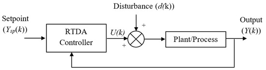
Figure 1.
General closed loop diagram with a robust, tracking, disturbance rejection and aggressiveness (RTD-A) controller.
- Predicting the process output;
- Updating the model prediction;
- Computing the control action.
Most of the processes can be represented in the form of the first order process with a dead time (FOPDT) model. It turns out to be very useful to investigate the system output because it has all the necessary components in the unambiguous form. At the first step, the higher order over-damped system transfer function reduced to the FOPDT model using different methods such as fraction incomplete, two-point and Skogestad in the Tool-I [28]. The FOPDT system output used in this paper is given in (1) [29]:
where K is the process gain, is the dead time or transportation lag, is the time constant, u(s) is the process input and y(s) is the process output. The discrete model for (1) is given in (2).
where,
- a = e−Δt/τ, Δt is the sampling time;
- b = K(1 − e−Δt/τ) and m = round(α/Δt).
From (2), the output prediction for the next m steps can be written as in (3) [11].
where,
- .
µ is the weighted sum of the past control action taken during the m period and u(k) is the current control action. There will be only one control u(k) allowed from the current time instant and is given in (4).
Equation (5) is obtained by considering the predicted process output over the next N-steps.
where,
The model prediction requires a model error that is decomposed into two parts such as the effect of model mismatch em(k) and unmeasured disturbance eD(k). Therefore, the total error is (7),
The estimate of eD(k) is given as (8).
where θR lies between 0 and 1. The controller has the robustness ability to handle the plant uncertainties. The future disturbance effect is predicted according to (9).
for , where .
Here θD is the disturbance rejection controller tuning parameter. Finally, by solving the (5) and (9) the updated N-step model output prediction is given by (10).
A plant with the setpoint trajectory has the control action to minimize the error. At a discrete time interval, the control action will be updated. If the desired final output is considered as yd(k), then the desired trajectory to follow y*(k) is given by (11).
The setpoint tracking tuning parameter θT is introduced, which varies from 0 to 1. The value of N will be calculated by the controller aggressiveness tuning parameter θA given in (12).
The RTD-A controller output u(k) is given in (13). The calculated controller output was applied to the plant. Where .
The controller output calculation was done in MATLAB. It was used to design a GUI tool described in Section 4.
2.1. Stability Analysis
2.1.1. State Variable Form
When the RTD-A controller based on the nominal model G(s) is implemented on the plant with model uncertainty (λ), the resulting closed-loop behavior may be represented in the discrete state-space form in (14) and (15) [13].
where X(k), yd, d and do are the state vector, setpoint, load disturbance and output disturbance respectively.
The control action u(k) is given by (16):
The characteristic equation of the closed loop system is given by (17):
where z is the z-transform variable, and, for closed-loop stability, all the roots of (17) must lie strictly inside the unit circle < 1.
The matrix R and vectors Q and S in (17) are:
where A, B, C, D, E, F and ζ are defined as follows:
2.1.2. Polynomial Form
The characteristic polynomial of the RTD-A controller in (18) can be written as in [14]:
where
The stability can be analyzed on the basis of the Jury’s test. A necessary condition for all the roots of the nth order polynomial to lie inside the unit circle is that:
where the coefficient c0 and cn can be calculated using (21) and (22).
The system will be stable if (23) and (24) is satisfied.
The closed loop stability in terms of the robustness tuning parameter θR can also be determined. The necessary condition is given in (25). The right-side term in (25) is defined as θref for simplicity.
The discussed necessary conditions in this section are used to check the stability of the liquid level control and pressure control in the evaluation section.
3. Tool Design
The flowchart shown in Figure 2 is the basic building of the tool designed. Each part of the flowchart was implemented in terms of GUI and the corresponding MATLAB functions were designed. There were four GUI tools, which were designed to work on the RTD-A controller and each tool had its own function. The output of one tool will be an input for another tool. The flowchart starts with the input from the user, the tool checks if the given transfer function is in the FOPDT model or not. If the transfer function is in FOPDT form, the user can proceed further with the desired tool designed in MATLAB. If the transfer function is of a higher order, then the user has to use the tool for model order reduction to obtain the FOPDT model.
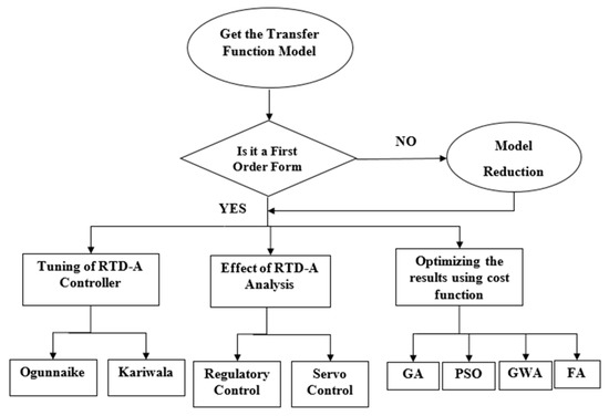
Figure 2.
Flowchart for the simulation tool design.
The main aim of the tool is to facilitate the user with all functions used for the RTD-A control scheme. After the final step, the user has the choice to select the analyzing tool. The GUI with RTD-A functionality will be acquired by calling the function name in the command window. The following subsections explain the working of the tool in detail.
3.1. Tool for Model Order Reduction (Tool-I)
It is mandatory to derive the first order process transfer function with/without dead time (when the provided transfer function has a higher order). The Tool-I is designed to reduce the over damped higher order transfer function into the FOPDT model. The required elements of the transfer function are stored in the workspace. This tool is composed of three methods for model order reduction that is as follows, the [4,30]:
- Skogestad method;
- Two point method;
- Fraction incomplete method.
3.2. Tool for Tuning RTD-A Parameter (Tool-II)
After calculating the FOPDT model, to calculate RTD-A tuning parameter the Tool-II was designed. This tool has a drop-down menu containing two methods for tuning [14].
- The Mukati–Ogunnaike method;
- The Kariwala method.
The user can select any one method and check the results with the given input (. The tool also enables the user to plot the closed loop response and compare the results. Each time the tool plots the response in a different color so that the user can easily identify the difference in two outputs. The tool has the option to switch the algorithm and check the response.
3.3. Tool for Analyzing the Effect of the RTD-A Parameter (Tool-III)
The RTD-A control scheme can work with the tuned parameters calculated from the “tune_RTD-A” function command. However, sometimes the user wants to adjust the tuning parameters in order to analyze the effect of each parameter on the process output. The Tool-III is used for adjusting the parameters manually and analyzing the results with a graphical representation. The tool can provide the following responses:
- Servo response (performance of the controller without disturbances);
- Regulatory response (performance of the controller considering only disturbances).
In order to analyze the system performance, the tool has the facility to check the performance for different set points. The user can pass in a maximum of three set points at different time instances. The Tool-III is also equipped with provision to add disturbance at a particular instant and time domain analysis with step response can be done. The tool is designed to take the values for K, τ and α from the workspace for the ease of the researcher.
The developed tool has the ability to handle the FOPDT transfer function model parameter values and to display the tuned values of the controller parameter. The effect of each tuning parameter (θR, θT, θD and θA) on the plant output is clearly explained by Ogunnaike and Srinivasan [13,31].
3.3.1. Effect of Robustness Parameter
θR parameter determines the controller robustness on the process output. The high open loop process gain causes for significant robustness in the face of process parameter uncertainty. It is desirable to have a negligible effect of parameter changes on the process output. The controller action is expected to be swift when is closer to unity and vice versa when it is near zero.
3.3.2. Effect of the Setpoint Tracking Parameter
θT is the parameter that deals with the controller setpoint tracking ability. It does not affect the closed loop stability. θT is chosen by considering the closed loop conditions. The error in the process output is determined by the tracking parameter. If the value of is close to 1, it leads to a sluggish response and vice versa when it is zero.
3.3.3. Effect of the Disturbance Rejection Parameter
θD is the parameter that deals with future conditions. Here, the disturbances are deliberated as a composite disturbance. It includes both process model mismatch and unmeasured disturbances. The controller will be more aggressive when θD is close to zero. If θD is closer to unity the disturbance effect will be changing into the future. Conversely, when θD is zero then the disturbance effect will remain constant throughout the system response.
3.3.4. Effect of the Aggressiveness Parameter
θA is the parameter associated with the prediction horizon N. The prediction horizon value provides information about how much the future output can be predicted. The controller will be more conservative when the tuning value is high. The RTD-A will be more conservative when compared to the PID controller. An N value is large when the tuning value is near one and it has a short prediction horizon when θA is close to zero [14].
3.4. Tool for Optimizing the RTD-A Controller Parameter (Tool-IV)
The Tool-IV is exclusively made for optimization, which can generate the ideal results of the tuning parameters (θR, θT, θD and θA) with the help of four different optimization algorithms. The algorithms are chosen arbitrarily. A cost function required for optimization can be chosen by selecting the “Get Cost” function. The main aim of the tool is to determine the optimal tuning parameters by minimizing the error between the actual process output and set-point. In order to minimize the cost function, the tool implements the intuitively chosen five heuristic algorithms such as:
- Galactic swarm optimization;
- Particle swarm optimization;
- Genetic algorithm;
- Firefly algorithm;
- Grey wolf algorithm.
3.4.1. Galactic Swarm Optimization
Galactic swarm optimization (GSO) is a new global optimization metaheuristic algorithm inspired by the motion of stars, galaxies and superclusters of galaxies under the influence of gravity. GSO employs multiple cycles of exploration and exploitation phases to strike an optimal trade-off between the exploration of new solutions and exploitation of existing solutions. In the explorative phase, different subpopulations independently explore the search space and in the exploitative phase, the best solutions of different subpopulations are considered as a superswarm and move towards the best solutions found by the superswarm. In this algorithm subpopulations as well as the superswarm are updated using the PSO algorithm. However, the proposed algorithm is quite general and any population based the optimization algorithm can be used instead of the PSO algorithm [32].
3.4.2. Particle Swarm Optimization
Particle swarm optimization (PSO) is an iterative algorithm to optimize a solution. This algorithm depends on the velocity and position equations. PSO needs the number of iterations and swarm sizes. A particle movement depends on the local best-cost particle. Other particles are nearer to local best approaches towards an optimal point. Finally, all the swarm approaches towards the global minimum and towards the best solution [33].
3.4.3. Genetic Algorithm
The genetic algorithm (GA) is a metaheuristic algorithm that depends on natural selection. The genetic algorithm works on three stages such as mutation, crossover and selection. In a genetic algorithm, individuals are generated randomly. This is an iterative process where the algorithm checks the fitness function. The fitness function produces the fitness value that represents the closeness towards optimized results. The genetic algorithm converges towards the values with optimized results [33]. In particular, the genetic algorithms avoid the local minimum efficiently [34].
3.4.4. Firefly Algorithm
The firefly algorithm (FFA) is a modified particle swarm algorithm. The distinguishable difference is that each particle in this algorithm is characterized by the brightness. Every individual firefly attracts all other fireflies. Attractiveness is proportional to their brightness. Here, the user has to give input of three parameters called α, β and γ. In this algorithm, α, β and γ are the mutation coefficient, attraction coefficient and the absorption coefficient respectively. This algorithm is similar to the particle swarm optimization algorithm when γ tends to zero. The number of swarms and iterations should be specified by the researcher [35].
3.4.5. Grey Wolf Algorithm (GWA)
This algorithm is one of the efficient and simple algorithms present in the research field. It mimics the technique of the grey wolf, which depends on leadership and a hunting mechanism. There are preys that are the food of wolves. The algorithm employs four grey wolves that are simultaneously working on three tasks that are searching, encircling and attacking prey [36].
All these tuning parameters will affect the final controller output. The optimal tuned values for the four parameters can be obtained by minimizing the suitable cost function. The controlled process response can be altered by adjusting the tuning parameters. The challenge in the optimal tuning of the RTD-A controller parameters is succeeded by the proposed tool.
The researchers have developed different methods for dealing with the controller tuning parameters. One such technique is the Ogunnaike tuning rule. It has one notable parameter called the composite parameter . It is given in (26):
where is the multiplicative factor, which is associated with process uncertainty and its value lies in the range of 0 to 1 for the FOPDT process model.
When the uncertainty parameter λ is added to the nominal plant model in (1), the plant parameters is defined in (27).
K0 = K(1 + λ), τ 0= τ(1 + λ) and α0 = α(1 + λ).
The equivalent discrete plant parameters is given in (28):
a0 = e−Δt/τ0, b0 = K0(1 − a0) and m0 = round(α0/Δt).
The plant output can be written as (29), where d is the disturbance.
yp(k) = a0yp(k − 1) + b0(u(k − m0 − 1) + d(k − m0 − 1)).
Similarly, the model output from (2) can be written as (30).
The model error e(k) in (31) is used in (7) to calculate the control action.
There are definite constraints on the tuning parameters with respect to the composite parameter. The Mukati–Ogunnaike tuning rule is presented in Table 1.

Table 1.
Mukati–Ogunnaike tuning rules [4].
The Kariwala, tuning rule is shown in Table 2. It is a semi-analytical tuning method. The tuning rules are obtained with the extensive experimental study on the different FOPDT transfer function [11].
Table 2.
Kariwala tuning rules [4,14].
The variety of the first order transfer function models is tested with robust stability analysis and the plant model mismatch using the Kariwala tuning method in the literature. Here, the researcher can observe that the tuning rule is transparent with respect to the controller performance features. The Kariwala tuning rule demonstrates the decent performance for a variety of processes. In some cases, Mukati–Ogunnaike tuning rules may lead to instability because of its inherent aggressiveness characteristics [14].
The model order reduction techniques, tuning rules and optimization algorithms discussed in this section were used to design a GUI tool in the tool description section. The proposed four tools are described with GUI in Section 4.
4. Tool Description
The FOPDT process model is required for the RTD-A controller design. If the process transfer function is not in the FOPDT form, then the model order reduction tool (Tool-I) will be used. The higher order process dynamics can be represented by the reduced model. The process reaction curve (PRC) method is one of the techniques to reduce the higher order process model into the first order model with dead time. It is considered to achieve a minimum integral squared error (ISE) in its ideal open loop step response. The GUI to reduce the higher order transfer function into the first order model is shown in Figure 3. Tool-I has the ability to reduce the higher order transfer function into the first order transfer function G. The proposed Tool-I has experimented on the liquid level process and it is discussed in the evaluation section [4].
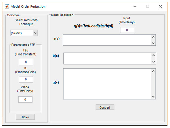
Figure 3.
Graphical user interface (GUI) for the model order reduction tool.
The outline of the method of model order reduction is given in (32).
where a(s) and b(s) is the numerator and denominator polynomial of the higher order process transfer function respectively and G(s) is the required reduced order model with or without dead time [4].
Generally, the system has some dead time when it is tested for robustness in a real-time environment. The Tool-I has the option to add a time delay while testing the system. Each order reduction method takes the dead time as one of the input and provides the required reduced order model output. Since the RTD-A controller depends on the process gain, process time constant and dead time, Tool-I basically separates all three parameters. It has also the facility with three model order reduction methods such as the Skogestad, two-point and fraction incomplete method. The chosen methods are effective for an over-damped process with dead time.
Next, this paper introduced the second tool that was designed for calculating the RTD-A controller tuning parameters. The GUI for the Tool-II is shown in Figure 4. This Tool-II was designed by considering the first order process with dead time models. It has the flexibility to tune the controller with both Ogunnaike and Kariwala tuning rules. The developed GUI has the provision for getting different inputs such as the sampling time (), process uncertainty parameter (), the process dead time (), composite noise factor () and process time constant () from the user. The user can choose one tuning rule from the selection menu. The calculated, tuning values will be shown in the RTD-A parameter portion of the Tool-II. If the user selects another tuning method from the menu during the next stint, the user has the provision to compare both results just by enabling the “Tune” button in operating the menu. Tool-II also has the facility to reset all the values to zero [20]. The tuning rules used in Tool-II are presented in Table 1 and Table 2.
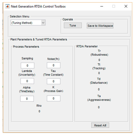
Figure 4.
For the RTD-A controller tuning tool.
In order to understand the effect of each controller parameter (θR, θT, θD and θA) on the process output the user has to change the value manually. The tool is made in such a way that the researcher has the facility to tune the controller manually with a slider option. The representation of Tool-III from the proposed tool is shown in Figure 5. The designed Tool-III has the facility to give a different set point at a different time instant and the user can perform a time domain analysis from the step response of the process.
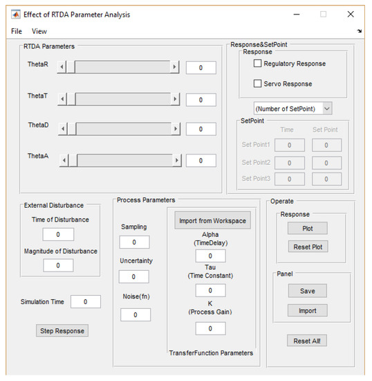
Figure 5.
GUI for analyzing the effect of the RTD-A parameter.
The disturbance can be added at a required instant and the user can check the effect of a tuning parameter on the process output with disturbance. Tool-III has also the provision to save current values of tuning parameters. After giving a set point to the tool, the user can change the values of the tuning parameters and check the tuning values in the slider display. The researcher can visually check the controller output and closeness to the ideal values. It can simulate all features of RTD-A by comparing the results in the same figure.
Manual tuning always lags behind tuning results with an optimization algorithm. The various control schemes like PID, model predictive control (MPC), fractional order PID (FOPID) and linear quadratic regulator (LQR) are available in the past. In all these algorithms many researchers have implemented optimization algorithms to get the optimum tuned results. In this paper, Tool-IV was proposed to find the optimal tuning values for the RTD-A control scheme. There were four algorithms included in the Tool-IV with the drop-down menu. The GUI is shown in Figure 6.
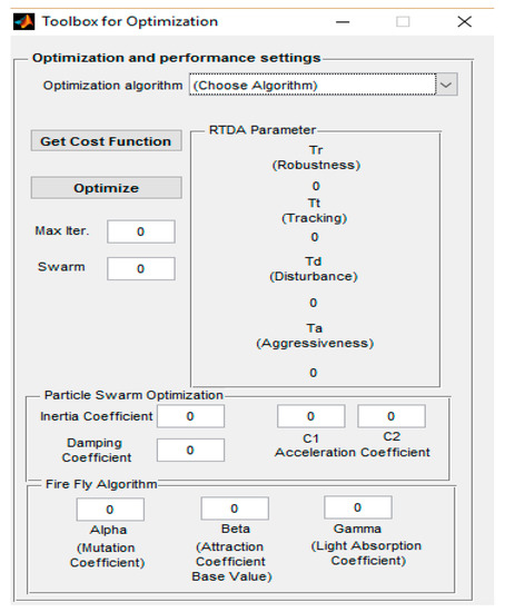
Figure 6.
GUI for the RTD-A controller parameter optimization tool.
The tool has the facility to give a path for the cost function. The main objective of the optimization algorithm is to minimize the cost function. The least cost corresponds to the optimized RTD-A values. After pressing the ’Optimize’ button, the user will have to wait for iterations to be completed. The least cost can be obtained in the MATLAB workspace. The Tool-II or III can be used to plot the closed loop process response with the optimized RTD-A parameter. The tools discussed in this section are experimented on two examples in the evaluation section.
5. Evaluation
In this section, the proposed tool has experimented on two different industrial processes such as the liquid level control and pressure control. The experiment was conducted on a personal computer running windows 10 pro 64-bit operating system with hardware configuration of Intel(R) Core(TM) i5-7200U CPU @ 2.5 GHz.
5.1. Example 1: Interacting a Two Tank Liquid Level System
The liquid level system shown in Figure 7 was considered for validating the proposed tool [4]. This is one of the commonly used real-time examples of the chemical process [37]. In a liquid level system, at steady state, the inflow rate and outflow rate are equal to . The flow rate between the two tanks is also zero and the heads of the tank 1 and tank 2 are equal to . At time t = 0, the inflow rate is changed from to , where q is small. The resulting changes in the heads () and flow rates () are assumed to be small as well. The capacitances of tank 1 and tank 2 are respectively. The resistance of the valve between the tanks is R1 and the outlet valve resistance is R2.
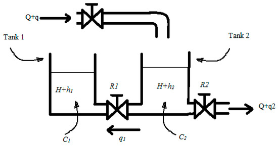
Figure 7.
Two tank liquid-level system [4].
From Figure 7, the transfer function between liquid level H2(s) and inlet flow rate Q(s) is derived and given in (33).
In order to understand the effect of the dead time in the process output, five seconds in dead time was introduced in the derived transfer function. Let R1 = R2 =1; C1 = C2 = 1. Now the resulting transfer function is given in (34):
It is a minimum phase stable system. Let us consider that the level control system is time critical and it is required to control the second tank level h2(t) by manipulating the inflow rate q(t). Since it is required to control h2(t) using the RTD-A controller, the actual system in Equation (34) is reduced into the FOPDT system. The three methods in Tool-I were used to obtain the FOPDT model of the process. The result of each method is presented in Table 3. The accuracy of the reduced model in terms of the integral square error (ISE) performance measure was also compared. It was found that the fraction incomplete method based model was more accurate for this interacting liquid level system. Hence, in this section, the remaining analysis was carried out with the obtained accurate reduced model in (35).
Table 3.
Performance comparison of order reduction techniques.
The open loop response of a reduced order model is displayed in Figure 8. The fraction incomplete method-based model response was very much closer to the actual second order process response than other methods [4]. The implementation of the RTD-A controller with a simulation tool on the liquid level control is shown in Figure 9. The performance of the RTD-A controller with two tuning algorithms and the PID controller was examined in controlling the h2(t) without uncertainties and disturbance. The structure of the PID controller transfer function used is given in (36). The PID tuning parameters proportional gain (KP), integral gain (KI), derivative gain (KD) and filter co-efficient (Tf) used in the simulation were determined using the auto tune function in MATLAB.
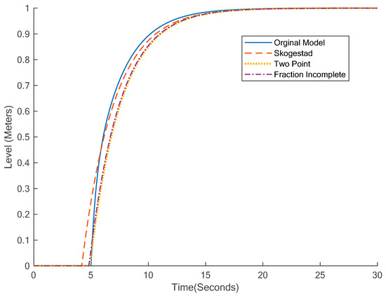
Figure 8.
Open-loop step response with reduced models.
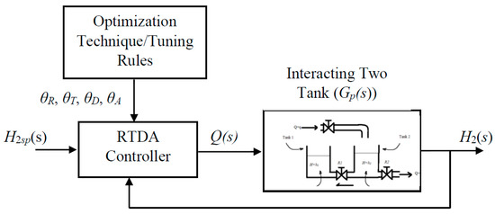
Figure 9.
Level control system with the RTD-A controller.
The tuning parameters for the process with uncertainty and disturbance using two tuning rules are given in Table 4. The sampling time of 0.1 s was considered in the controller implementation. The PID auto tuned values were KP = 0.496, KI = 0.116, KD = −0.857 and Tf = 0.128. The setpoint for h2(t) was considered as one meter. The servo response with the PID and RTD-A for zero uncertainty and zero disturbance is shown in Figure 10. Similarly, the servo response with RTD-A tuned using the optimization algorithm is shown in Figure 11.
Table 4.
Example 1: Tuning parameters with two tuning methods [4].
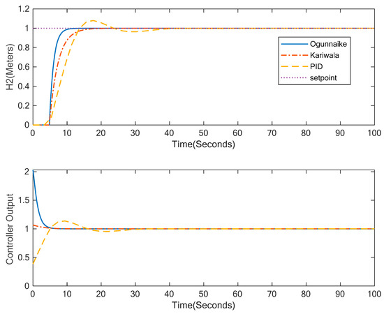
Figure 10.
Example 1: Servo response with the RTD-A controller using two tuning methods.
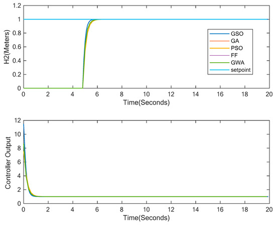
Figure 11.
Example 1: Servo response with the RTD-A controller using optimization algorithms.
The efficiency of the proposed tool was examined by adding the uncertainty parameter () and disturbance to the plant. The RTD-A and PID controlled servo response with disturbance and uncertainty are shown in Figure 12 and Figure 13. The RTD-A controller requires values for the sampling time, noise and uncertainty parameter as an input. The tool II was provided with the same input parameters for comparing the two different tuning algorithms. Whenever the user chooses the tuning rule, the tool will acclimate to the chosen tuning rule. In Figure 12, the response with the Ogunnaike tuning method was more susceptible to noise and also it exhibited a more aggressive controller response. It had some overshoot as compared with the Kariwala tuning method. The process response with the first method deviated more from the setpoint and this deviation increased further with the increase in the uncertainty parameter (λ). The Kariwala, tuning method was more flexible with respect to the controller aggressiveness and uncertainty. The response with PID had more rise and settling time with less overshoot and control variation than the Ogunnaike method. In Figure 13 the servo response with optimal tuned parameters after adding uncertainty is shown.
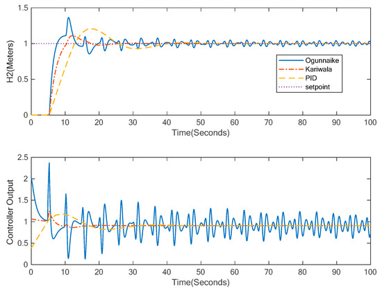
Figure 12.
Example 1: Servo response with the RTD-A controller with disturbance and uncertainties.
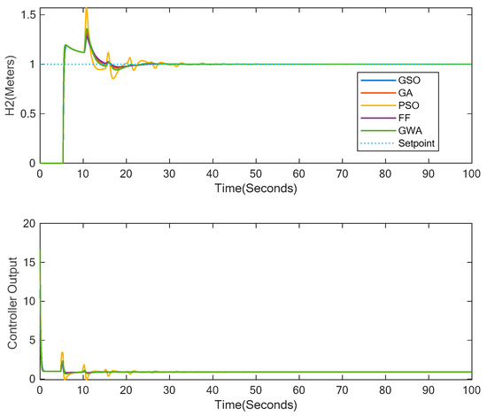
Figure 13.
Example 1: Servo response with the RTD-A controller with uncertainty using optimization algorithms.
The disturbance rejection ability of the RTD-A controller was experimented and the regulatory response without optimally tuned parameters is shown in Figure 14. In Figure 15, the response with disturbance rejection is shown for some optimally tuned values. The disturbance of 20% of setpoint was applied to the process at 50 s. It was found that all the controllers were able to reject the disturbance effect on the process output.
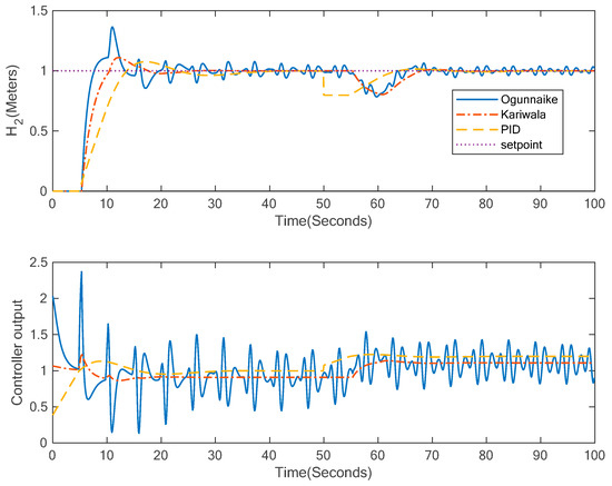
Figure 14.
Example 1: Regulatory response with the RTD-A controller using tuning rules and proportional integral derivative (PID).
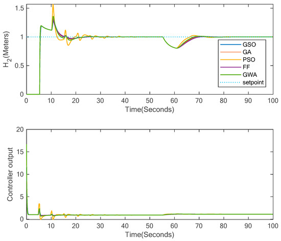
Figure 15.
Example 1: Regulatory response with the RTD-A controller using optimization algorithms.
The unit step change in setpoint was applied to the closed loop system and time response was obtained. The time domain specifications could be calculated from the step response of the closed loop system using the stepinfo command in MATLAB. The RTD-A controller performance for two tuning rules and optimal tuning was compared in terms of the integral absolute error (IAE) and other time domain specifications with PID performance and it is presented in Table 5. In this example performance with RTD-A was better than PID. Between the first two tuning rules, the Kariwala tuning rule-based process response had a good performance compared to the Ogunnaike tuning method excluding the rise time. However, in the overall comparison the firefly algorithm-based result was slightly better than the other methods.
Table 5.
Example 1: Performance comparison with different tuning methods.
The execution time of the RTD-A and PID controller implementation for the servo response of level control without uncertainty was 0.034279 s and 0.062699 s respectively. Similarly, 0.070815 s and 1.048175 s with 10% uncertainty on process parameters when the simulation time was 100 s.
The Tool-III was applied to the liquid level control system and the effect of the tuning parameter on the process output was analyzed. Each parameter can be changed with the slider and even small changes in the process output can be realized. In Example 1, the θR, θT and θA values were changed and the output of the plant with respect to time was plotted. The output of Tool-III for Example 1 with sequential changes in setpoints (SP = 1 m, SP = 5 m and SP = 2 m) is shown in Figure 16, Figure 17 and Figure 18.
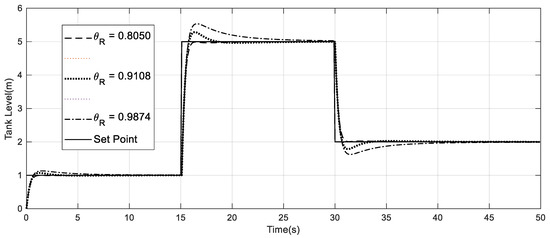
Figure 16.
Response to Tool–III for changing the θR parameter.
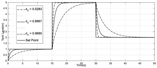
Figure 17.
Response to Tool III for changing the θT parameter.
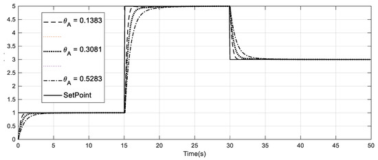
Figure 18.
Response to Tool III for changing the θA parameter.
In Figure 16 the process response rise time decreased and settling time increased as the θR approaches unity. The response was robust as the θR value was small. The effect of the setpoint tracking parameter on the process output is shown in Figure 17. The response became sluggish and the settling time increased as the θT approached unity. In Figure 18, as the θA value approached 1, the response was moving away from the desired set point. Therefore, for the lesser value of θA, the process output was closer to the desired level. Similarly, the process output reached the set point very quickly without overshoot as the parameter θA was small.
Tool-IV experimented with the liquid level control system. The objective of the optimal control problem was to minimize the error between the setpoint (yd) and actual process output (yp). Therefore, the integral absolute error (IAE) cost function in (37) was chosen for both example 1 and example 2. During this optimal tuning process, an output disturbance was also considered with ±10% random variation.
The number of iterations and swarm size used in the optimization is tabulated in Table 6. The additional parameters required for PSO and firefly algorithms are listed in Table 7. The algorithm parameters were chosen based on a certain number of trial runs for the smooth convergence. The same settings were used in the Example 2 experimentation. The optimal tuned values obtained from the tool are listed in Table 8. These values could be used in Tool-II to plot the closed loop response when needed. Here, these values were used to control the liquid level process. The liquid level response is shown in Figure 11 and Figure 13. As mentioned earlier the overall performance was compared with other methods in Table 5.
Table 6.
Iteration and swarm size used in the optimization algorithm.
Table 7.
Additional parameters for galactic swarm optimization (GSO), PSO and firefly.
Table 8.
Example 1: Tuning parameters with an optimization tool.
5.1.1. Example 1: Closed Loop Stability Analysis
The stability of the closed loop liquid level control and pressure control with the RTD-A controller was checked according to Ogunnaike et al. and Kariwala et al. [11,12]. The stability analysis concept in the state variable form was discussed in Section 2.1.1. It is necessary that the roots of the characteristics equation in (17) should lie within the unit circle for closed loop stability. The roots of the liquid level control characteristic equation in the state variable form were calculated using (17) for different tuning methods and listed in Table 9. The location of roots in the z-plane was plotted and shown in Figure 19. Since all the roots were located inside the unit circle, the system was stable for all tuning methods.
Table 9.
Example 1: Roots with different tuning methods.
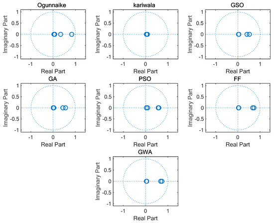
Figure 19.
Example 1: z-plane plot for the roots of the characteristic equation.
The stability could also be analyzed on the basis of the Jury’s stability criterion discussed in 2.1.2. The coefficients c0 and cn were calculated using (21) and (22). The value of the polynomial P(z) when z = 1 and z = −1 was calculated according to (18). The θref value also was calculated to check the stability in terms of θR using (25). The calculated values are tabulated in Table 10. The value of cn = 51,164, θref = 0.07 and the order of P(z) was an even number. The necessary conditions in (20), (23), (24) and (25) were checked for stability. It was found that all the conditions were satisfied for closed loop stability for the calculated tuning values. Therefore, the designed RTD-A controller ensured closed loop stability in liquid level control. A similar analysis was done for pressure control in Section 5.2.1.
Table 10.
Example 1: Jury’s stability test for liquid level control (cn = 5.1164e + 04 and θref = 0.07).
The open loop gain margin (GM) of the liquid level process was 4.1 dB and the closed loop GM with PID was 5.86 dB. Thus the closed loop stability with PID would be ensured by choosing the proportional gain value less than open loop gain margin value.
5.2. Example 2: Pressure Control System
A pressure control station is shown in Figure 20. The FOPDT model for pressure process was found using the black box modeling technique [38]. The corresponding first order process model is given in (38):
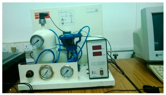
Figure 20.
Pressure control station [38].
The servo performance of the real-time system model without uncertainty was analyzed with the proposed tool and PID controller. The implementation of the controller with the simulation tool on pressure control is shown in Figure 21. The tank pressure P(t) was to be controlled by adjusting the outlet flow air flowrate Qout(t). All four parameters were tuned using the Tool-II and -IV. The tuned values are listed in Table 11 and Table 12 respectively. The control objective of the optimal control problem was to reduce the error between the desired pressure and actual pressure. The IAE cost function given in (37) was used to determine the optimal tuning values of RTD-A.
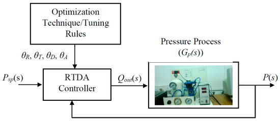
Figure 21.
Pressure control station with the RTD-A controller.
Table 11.
Example 2: Tuning parameters with tuning methods.
Table 12.
Example 2: Tuning parameters with an optimization tool.
During this optimal tuning process, an output disturbance was also considered with ±10% random variation.
The PID controller tuning values obtained from the auto tune function in MATLAB were KP = 1.373, KI = 0.143, KD = −0.178 and the filter co-efficient (Tf) = 0.115.
5.2.1. Example 2: Closed Loop Stability Analysis
The roots of the characteristics equation of pressure control process were calculated for different tuning methods using (17) and listed in Table 13. The location of roots in the z-plane is shown in Figure 22. It was observed that all the roots were located inside the unit circle. As mentioned in Section 5.1.1, the Jury’s stability test was performed on the pressure control process. The value of P(z) for z = 1 and z = −1, θref, coefficients c0 and cn were calculated using (18), (21), (22) and (25). The values are tabulated in Table 14. The calculated values were checked for stability necessary conditions in (20) and (23)–(25). The value of cn = 1.5929e + 07, θRef = 0.3295 and the order of P(z) was an odd number.
Table 13.
Example 2: Closed loop roots with different tuning methods.
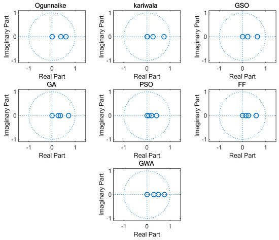
Figure 22.
Example 2: z-plane plot for the roots of the characteristic equation.
Table 14.
Example 2: Jury’s stability test for pressure control (cn = 1.5929 × 10⁷ and θRef = 0.3295).
It was found that the RTD-A tuning parameter satisfied all the necessary conditions for the closed loop stability. It is guaranteed that pressure control will be stable with the RTD-A controller.
The gain margin of the open loop pressure system was 35.3 dB and the closed loop gain margin with PID was 24.1 dB. The closed loop stability with PID is guaranteed if the proportional gain is chosen less than the maximum open loop gain margin value.
The setpoint 53 psi was considered for the pressure control process. The RTD-A and PID controller tuned values were used to control the pressure process. The servo response with RTD-A for a different tuning method and PID is shown in Figure 23. The pressure response with RTD-A using optimization algorithms is shown in Figure 24.
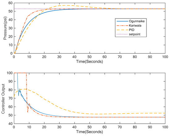
Figure 23.
Comparison of the servo response for the pressure control station with two tuning rules and PID.
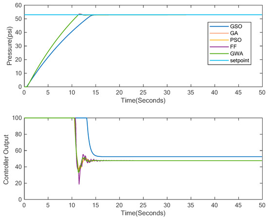
Figure 24.
Comparison of the servo response for the pressure control station with optimization algorithms.
The execution time of RTD-A and PID controller implementation for the servo response of pressure control was 0.047388 s and 1.643077 s respectively when the simulation time was 100 s and sampling time was 0.1 s.
The regulatory response of the pressure control process without optimally tuned values and with optimally tuned values is shown in Figure 25 and Figure 26 respectively. The setpoint 50 psi was considered in the investigation of disturbance rejection ability. The 10% of setpoint was applied as the disturbance to the process at 50 s in Figure 25 and at 25 s in Figure 26. The disturbance rejection ability of the optimally tuned RTD-A controller was better than the other method.
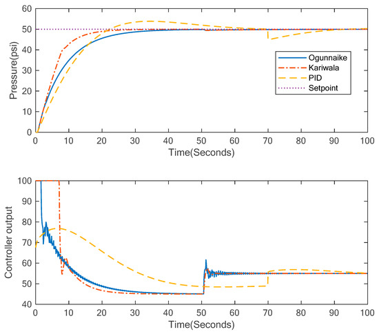
Figure 25.
Example 2: Regulatory response for the pressure control station with tuning rules and PID.
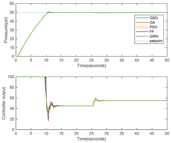
Figure 26.
Example 2: Regulatory response for the pressure control station with optimization algorithms.
The overall performance comparison for example 2 is done in Table 15. There was no noticeable difference in the performance of pressure control among the optimally tuned responses excluding GSO. The pressure process works better with the optimal tuning method in terms of IAE and other time domain performance measures. The response with the Kariwala tuning method took longer for the settling time and less rise time than the Ogunnaike tuning. A steady state error was almost zero in all the methods. There was a minimum overshoot in the response with the optimal tuned values, but the percentage overshoot in the Ogunnaike and Kariwala method was absolutely zero. The performance with RTD-A was better than PID in pressure control.
Table 15.
Example 2: Performance comparison of different tuning methods and PID.
Overall, in a liquid level control system, the firefly optimization tuned response was better than other methods. The genetic algorithm tuned response was better than other methods excluding percentage overshoot in the pressure control process.
6. Conclusions
The RTD-A controller is evolving very fast and can be used as an alternative for the classical PID controller. Since RTD-A has an independent tuning parameter for robustness it can handle the systems with uncertain behavior. The proposed simulation tool is the very basic implementation of the RTD-A controller. This tool can be used to approximate an over-damped higher order transfer function into a FOPDT system. Therefore, the proposed tool can be implemented on any higher order processes with or without dead time. The industrial processes can adopt this RTD-A controller with more flexibility. In the case study, the proposed tool had experimented on an interacting two tank liquid level process and a pressure control application. The optimization tool was tested in both cases and obtained the optimized results for the controller parameters under different optimization algorithms. In order to understand the effect of the changes in each tuning parameter on the plant output, a separate tool was developed for the RTD-A tuning parameter analysis and it was experimented on the interacting liquid level process. The closed loop stability of the liquid level control and pressure control was checked in the state variable form and also using the Jury’s stability criterion. It was found that the controller guaranteed the closed loop stability. Finally, the closed loop process performance with the optimal tuned RTD-A controller using the firefly algorithm was better than other methods in terms of IAE. The Kariwala tuning rule was also observed to be superior in terms of the settling time and overshoot performance measure in the liquid level control. Similarly, the optimization algorithms-based controller gave better performance in terms of IAE and other time domain specifications while controlling the pressure process station. The limitation of the proposed tool, it is not suitable for experimenting with the unstable processes and the multi input–multi output processes. It was also assumed that the process behavior could be adequately described by a FOPTD model. In the future, the proposed tool could be enhanced by adding other optimization algorithms, frequency domain analysis and multi-input multi-output process controlling ability. The facility could be added in the proposed tool to study the effect of optimization algorithm’s random parameters on the process output. The proposed tool “RTDA_Toolbox” could be downloaded from the link in https://drive.google.com/open?id=14GcTMwft7pn3bLcxOTvfX7_MNIDdlBLu.
Author Contributions
V.B. proposed the simulation tool concept and implemented the model order reduction and tuning of controller for different processes and wrote the paper; S.U. did the controller performance analysis and P.A. proposed the optimal tuning and edited the paper.
Funding
This research was funded by VIT, Vellore.
Acknowledgments
The authors like to express their sincere gratitude to the Process control Laboratory and School of Electrical Engineering, VIT, Vellore for giving opportunity to do the project in this area. Finally authors acknowledge the Renewable Energy Lab, Prince Sultan University, Riyadh for providing technical guidance for the execution of these research activities.
Conflicts of Interest
The authors declare no conflict of interest.
References
- Ruz, M.L.; Garrido, J.; Vazquez, F.; Morilla, F. Interactive Tuning Tool of Proportional-Integral Controllers for First Order Plus Time Delay Processes. Symmetry 2018, 10, 569. [Google Scholar] [CrossRef]
- Lequin, O.; Gevers, M.; Mossberg, M.; Bosmans, E.; Triest, L. Iterative feedback tuning of PID parameters: Comparison with classical tuning rules. Control Eng. Pract. 2003, 11, 1023–1033. [Google Scholar] [CrossRef]
- Dai, A.; Zhou, X.; Liu, X. Design and Simulation of a Genetically Optimized Fuzzy Immune PID Controller fora Novel Grain Dryer. IEEE Access 2017, 5, 14981–14990. [Google Scholar] [CrossRef]
- Bagyaveereswaran, V.; Suryawanshi, S.; Arulmozhivarman, P. RTD-A controller toolbox for MATLAB. In Proceedings of the 2017 Innovations in Power and Advanced Computing Technologies (i-PACT), Vellore, Tamilnadu, India, 21–22 April 2017. [Google Scholar]
- Ender, D.B. Process Control Performance: Not as Good as You Think. Control Eng. 1993, 40, 180–190. Available online: https://www.academia.edu/1340822/Process_control_performance_Not_as_good_as_you_think (accessed on 20 May 2019).
- Chen, Q.; Tan, Y.; Li, J.; Mareels, I. Decentralized PID Control Design for Magnetic Levitation Systems Using Extremum Seeking. IEEE Access 2018, 6, 3059–3067. [Google Scholar] [CrossRef]
- Desborough, L.; Miller, R. Increasing customer value of industrial control performance monitoring -Honeywell experience. In AIChE Symposium Series 326; American Institute of Chemical Engineers: New York, NY, USA, 2002; pp. 172–192. [Google Scholar]
- Kristiansson, B.; Lennartson, B. Robust and optimal tuning of PI and PID controllers. IEEE Proc. Control Theory Appl. 2002, 149, 17–25. [Google Scholar] [CrossRef]
- Hugo, A. Limitations of Model Predictive Controllers. Hydrocarb. Process. 2000, 79, 83–88. [Google Scholar]
- Kaya, I. IMC based automatic tuning method for PID controllers in a Smith predictor configuration. Comput. Chem. Eng. 2004, 28, 281–290. [Google Scholar] [CrossRef]
- Mukati, K.; Ogunnaike, B. Stability analysis and tuning strategies for a novel next generation regulatory controller. In Proceedings of the 2004 American Control Conference, Boston, MA, USA, 30 June–2 July 2004; Volume 5, pp. 4034–4039. [Google Scholar]
- Ogunnaike, B.A.; Mukati, K. An alternative structure for next generation regulatory controllers: Part I: Basic theory for design, development and implementation. J. Process Control 2006, 16, 499–509. [Google Scholar] [CrossRef]
- Mukati, K.; Rasch, M.; Ogunnaike, B.A. An alternative structure for next generation regulatory controllers. Part II: Stability analysis, tuning rules and experimental validation. J. Process. Control. 2009, 19, 272–287. [Google Scholar] [CrossRef]
- Sendjaja, A.Y.; Ng, Z.F.; How, S.S.; Kariwala, V. Analysis and Tuning of RTD-A Controllers. Ind. Eng. Chem. Res. 2011, 50, 3415–3425. [Google Scholar] [CrossRef]
- Aleksei, T.; Eduard, P.; Juri, B. A flexible MATLAB tool for optimal fractional-order PID controller design subject to specifications. In Proceedings of the 31st Chinese Control Conference, Hefei, China, 25–27 July 2012; pp. 4698–4703. [Google Scholar]
- Currie, J. jMPC Toolbox v3. 11 Users Guide. In Industrial Information & Control Centre; AUT University: Auckland, New Zealand, 2011. [Google Scholar]
- Bagyaveereswaran, V.; Mathur, T.D.; Gupta, S.; Arulmozhivarman, P. Performance comparison of next generation controller and MPC in real time for a SISO process with low cost DAQ unit. Alex. Eng. J. 2016, 55, 2515–2524. [Google Scholar] [CrossRef]
- Morales, D.C.; Jimenez-Hornero, J.E.; Vazquez, F.; Morilla, F. Educational Tool for Optimal Controller Tuning Using Evolutionary Strategies. IEEE Trans. Educ. 2012, 55, 48–57. [Google Scholar] [CrossRef]
- Bang, H.; Lee, Y.S. Implementation of a Ball and Plate Control System Using Sliding Mode Control. IEEE Access 2018, 6, 32401–32408. [Google Scholar] [CrossRef]
- Holland, O.T.; Marchand, P. Graphics and GUIs with MATLAB; Chapman and Hall/CRC Press: Boca Raton, FL, USA, 2002. [Google Scholar]
- Templos-Santos, J.L.; Aguilar-Mejia, O.; Peralta-Sanchez, E.; Sosa-Cortez, R. Parameter Tuning of PI Control for Speed Regulation of a PMSM Using Bio-Inspired Algorithms. Algorithms 2019, 12, 54. [Google Scholar] [CrossRef]
- Fan, Y.; Shao, J.; Sun, G. Optimized PID Controller Based on Beetle Antennae Search Algorithm for Electro-Hydraulic Position Servo Control System. Sensors 2019, 19, 2727. [Google Scholar] [CrossRef] [PubMed]
- Wang, R.; Tan, C.; Xu, J.; Wang, Z.; Jin, J.; Man, Y. Pressure Control for a Hydraulic Cylinder Based on a Self-Tuning PID Controller Optimized by a Hybrid Optimization Algorithm. Algorithms 2017, 10, 19. [Google Scholar] [CrossRef]
- Bilal, H. Abed-alguni, Island-based cuckoo search with highly disruptive polynomial mutation. Int. J. Artif. Intell. 2019, 17, 57–82. [Google Scholar]
- Soares, A.; Râbelo, R.; Delbem, A. Optimization based on phylogram analysis. Expert Syst. Appl. 2017, 78, 32–50. [Google Scholar] [CrossRef]
- Shams, M.; Rashedi, E.; Dashti, S.M.; Hakimi, A. Ideal gas optimization algorithm. Int. J. Artif. Intell. 2017, 15, 116–130. [Google Scholar]
- Precup, R.E.; David, R.C. Nature-Inspired Optimization Algorithms for Fuzzy Controlled Servo Systems, 1st ed.; Elsevier: Oxford, UK, 2019. [Google Scholar]
- Skogestad, S. Simple analytic rules for model reduction and PID controller tuning. J. Process. Control. 2003, 13, 291–309. [Google Scholar] [CrossRef]
- Leite, M.S.; Araújo, P.J. Relay Methods and Process Reaction Curves: Practical Applications; In Tech Open: Rijeka, Croatia, 2012; pp. 248–258. [Google Scholar]
- Jose, A. Romagnoli, and Ahmet Palazoglu. In Introduction to Process Control; CRC Press: Boca Raton, FL, USA, 2005. [Google Scholar]
- Srinivasan, K.; Anbarasan, K. Fuzzy scheduled RTD-A controller design. ISA Trans. 2013, 52, 252–267. [Google Scholar] [CrossRef] [PubMed]
- Muthiah-Nakarajan, V.; Noel, M.M. Galactic Swarm Optimization: A new global optimization metaheuristic inspired by galactic motion. Appl. Soft Comput. 2016, 38, 771–787. [Google Scholar] [CrossRef]
- Poli, R.; Kennedy, J.; Blackwell, T. Particle swarm optimization. Swarm Intell. 2007, 1, 33–57. [Google Scholar] [CrossRef]
- Visioli, A. Optimal tuning of PID controllers for integral and unstable processes. IEEE Proc. Control Theory Appl. 2001, 148, 180–184. [Google Scholar] [CrossRef]
- Yang, X.S. Firefly algorithms for multimodal optimization. In Proceedings of the International Symposium on Stochastic Algorithms, Sapporo, Japan, 26–28 October 2009; pp. 169–178. [Google Scholar]
- Mirjalili, S.; Mirjalili, S.M.; Lewis, A. Grey wolf optimize. Adv. Eng. Softw. 2014, 69, 46–61. [Google Scholar] [CrossRef]
- Ogata, K. Control System Dynamics, 4th ed.; Pearson Education Inc.: Upper Saddle River, NJ, USA, 2004; pp. 155–156. [Google Scholar]
- Bayaveereswaran, V.; Wilfred, K.J.N.; Sreeraj, S.; Vijay, B. System Identification from step input using Integral equation. Int. J. Appl. Eng. Res. 2013, 8, 2165–2169. [Google Scholar]
© 2019 by the authors. Licensee MDPI, Basel, Switzerland. This article is an open access article distributed under the terms and conditions of the Creative Commons Attribution (CC BY) license (http://creativecommons.org/licenses/by/4.0/).