Aiding Dictionary Learning Through Multi-Parametric Sparse Representation


Abstract
1. Introduction
- (i)
- The offline stage: find the way in which the optimal solution depends on parameter and store this information for later use in the online stage;
- (ii)
- The online stage: for the current value of , retrieve and apply the a priori computed solution.
- (i)
- The cost from the constrained optimization problem is rank-deficient (the dictionary is over-determined which means that the quadratic cost is defined by a semi-definite matrix);
- (ii)
- The norm used here (as a relaxation from the sparse restriction induced by the norm) leads to a very-particular set of linear constraints (they define a cross-polytope, whose structure influences the optimization problem formulation [11]).
- (i)
- The first issue requires a careful decomposition of the matrices (in order to avoid degeneracy in the formulations [12]); the upshot is that the particular KKT representation appears in a simple form (which allows simple matrix decompositions).
- (ii)
- The second requires to consider a vertex-representation of the cross-polytope (as this is a more compact representation than its equivalent half-space representation [13]). In general, the opposite is true: to a reasonable number of linear inequalities corresponds a significantly larger number of vertices. Thus, most if not all of space partitioning induced by the multi-parametric representation exploit the “half-space” description of the feasible domain [9].
- (iii)
- We highlight a compact storage and retrieval procedure (which exploits the symmetry of the cross-polytope domain) with the potential to significantly reduce the numerical issues.
2. The Dictionary Learning Problem
| Algorithm 1: Alternate optimization dictionary learning. |
 |
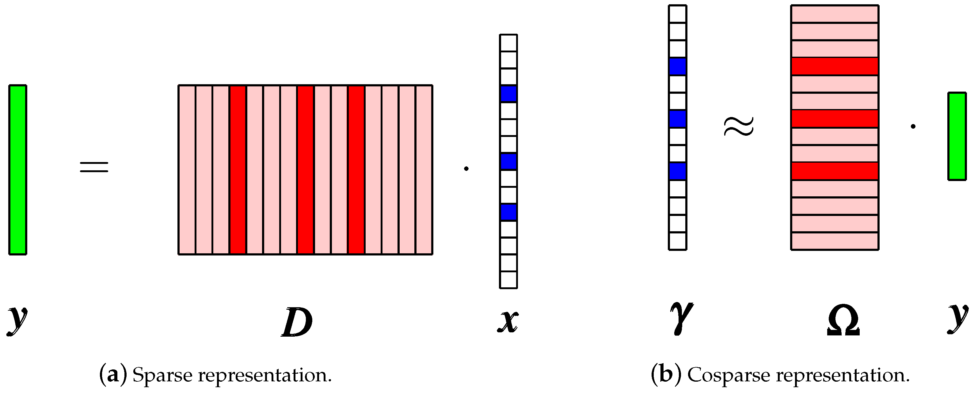
The Cosparse Model
3. Analysis of the Multi-Parametric Formulation Induced by the DL Problem
- (i)
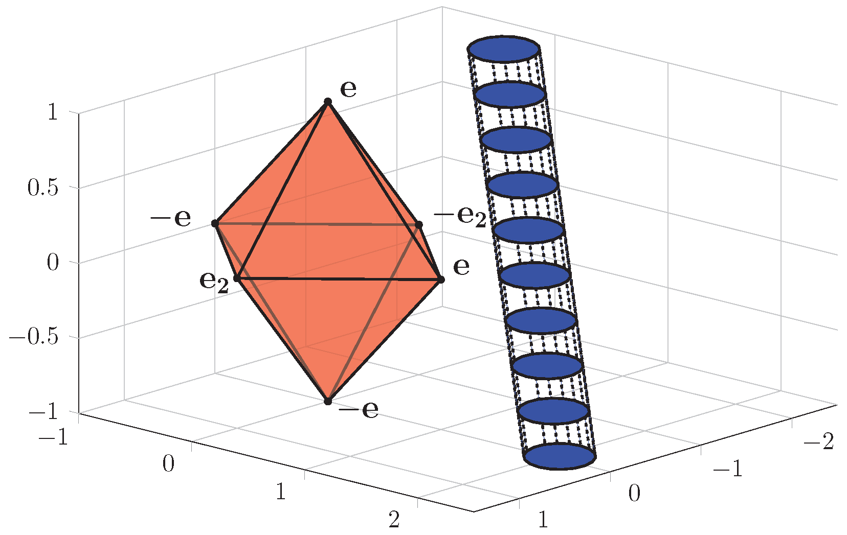
- The norm constraint characterizes a scaled and/or projected cross-polytope;
- (ii)
- The cost is affinely parametrized after parameter .
3.1. Geometrical Interpretation of the Norm
3.2. Karush–Kuhn–Tucker Form
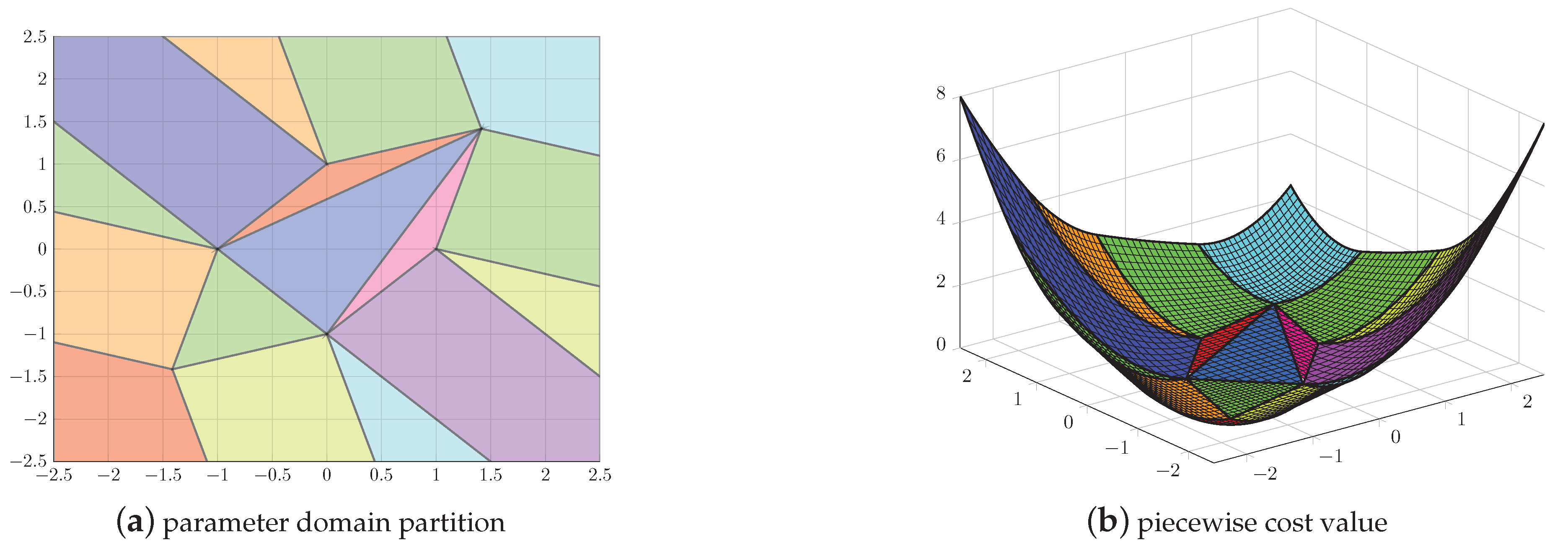
3.3. Multi-Parametric Interpretation
- (i)
- We obtain from (20b) as a function of and ;
- (ii)
- We introduce it in (20a) and obtain as an affine form of ;
- (iii)
- We go back in (20b), replace the now-known and obtain as an affine form of .
3.4. Illustrative Example
4. Integration of the Multi-Parametric Formulation in the Representation Problem
4.1. Multi-Parametric Formulations for the Sparse and Cosparse Representations
4.2. The Enumeration Roadblock
| Algorithm 2: Multi-parametric implementation of the sparse problem. |
 |
- (i)
- Only a single representative of the same family of active constraints has to be stored (Step 6 of Algorithm 2); the remaining variations may be deduced by multiplying with suitable ;
- (ii)
- The inclusion test (Step 3 of Algorithm 2) has to account for the sign permutations; this can be done, e.g., by checking whether holds. We denoted with ‘⊙’ the elementwise product and with the selection of (out of ) rows which correspond to the ones appearing in . Recall that weights come in pairs (since they are attached to the unit vectors ). This means that in a pair of indices there can be at most an active constraint (either the i-th or the -th). Thus, whenever we permute the signs we, in fact, switch these indices between the active and inactive sets.
4.3. On the Multi-Parametric Interpretation of the ‘Given Approximation Quality’ Case
- (i)
- The gradient is not well defined in inflexion points (where at least one of the vector’s components is zero); this requires the use of the ‘sub-gradient’ notion which is set-valued (29a) becomes ‘’, where
- (ii)
- The problem may be relatively large (depending on the number of inequalities used to over-approximate the initial quadratic constraint).
5. Results
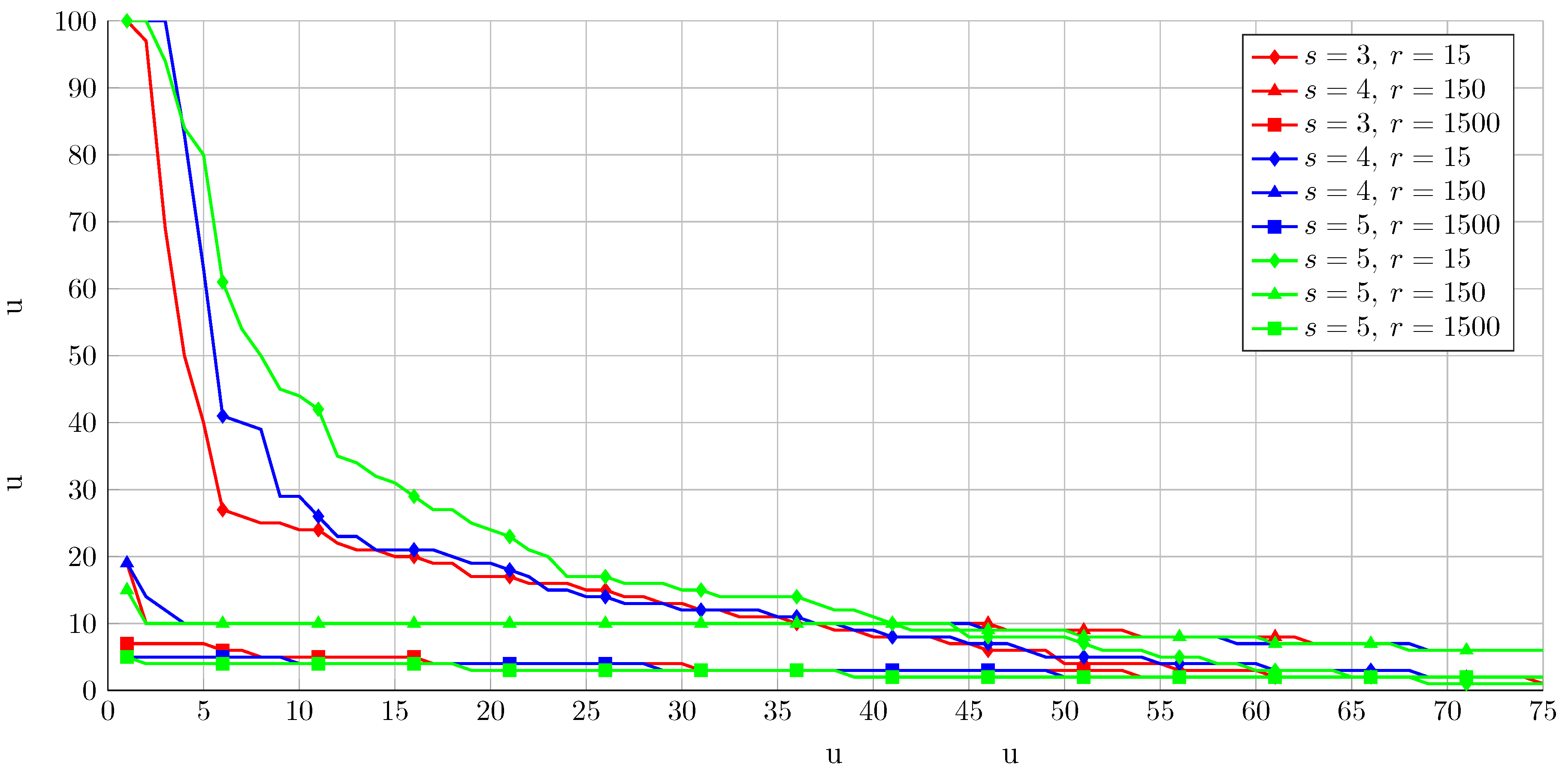
5.1. Synthetic Data
5.2. Water Networks
5.3. Images
6. Conclusions and Future Directions
Supplementary Materials
Author Contributions
Funding
Conflicts of Interest
References
- Elad, M. Sparse and Redundant Representations: From Theory To Applications in Signal and Image Processing; Springer Science & Business Media: Berlin, Germany, 2010. [Google Scholar]
- Fletcher, R. Practical Methods of Optimization; John Wiley & Sons: Hoboken, NJ, USA, 2013. [Google Scholar]
- Li, Z.; Ierapetritou, M.G. A method for solving the general parametric linear complementarity problem. Ann. Oper. Res. 2010, 181, 485–501. [Google Scholar] [CrossRef]
- Mönnigmann, M.; Jost, M. Vertex based calculation of explicit MPC laws. In Proceedings of the 2012 American Control Conference (ACC), Montreal, QC, Canada, 27–29 June 2012; pp. 423–428. [Google Scholar]
- Herceg, M.; Jones, C.N.; Kvasnica, M.; Morari, M. Enumeration-based approach to solving parametric linear complementarity problems. Automatica 2015, 62, 243–248. [Google Scholar] [CrossRef]
- TøNdel, P.; Johansen, T.A.; Bemporad, A. An algorithm for multi-parametric quadratic programming and explicit MPC solutions. Automatica 2003, 39, 489–497. [Google Scholar] [CrossRef]
- Tøndel, P.; Johansen, T.A.; Bemporad, A. Evaluation of piecewise affine control via binary search tree. Automatica 2003, 39, 945–950. [Google Scholar] [CrossRef]
- Bemporad, A. A multiparametric quadratic programming algorithm with polyhedral computations based on nonnegative least squares. IEEE Trans. Autom. Control 2015, 60, 2892–2903. [Google Scholar] [CrossRef]
- Alessio, A.; Bemporad, A. A survey on explicit model predictive control. In Nonlinear Model Predictive Control; Springer: Berlin, Germany, 2009; pp. 345–369. [Google Scholar]
- Jones, C.N.; Morrari, M. Multiparametric linear complementarity problems. In Proceedings of the 45th IEEE Conference on Decision and Control, San Diego, CA, USA, 3–15 December 2006; pp. 5687–5692. [Google Scholar]
- Coxeter, H.S.M. Regular Polytopes; Courier Corporation: Chelmsford, MA, USA, 1973. [Google Scholar]
- Ahmadi-Moshkenani, P.; Johansen, T.A.; Olaru, S. On degeneracy in exploration of combinatorial tree in multi-parametric quadratic programming. In Proceedings of the 2016 IEEE 55th Conference on Decision and Control (CDC), Las Vegas, NA, USA, 12–14 December 2016; pp. 2320–2326. [Google Scholar]
- Henk, M.; Richter-Gebert, J.; Ziegler, G.M. 16 basic properties of convex polytopes. In Handbook of Discrete and Computational Geometry; CRC Press: Boca Raton, FL, USA, 2004; pp. 255–382. [Google Scholar]
- Jost, M. Accelerating the Calculation of Model Predictive Control Laws for Constrained Linear Systems. 2016. Available online: https://hss-opus.ub.ruhr-uni-bochum.de/opus4/frontdoor/index/index/docId/4568 (accessed on 27 June 2019).
- Dumitrescu, B.; Irofti, P. Dictionary Learning Algorithms and Applications; Springer: Berlin, Germany, 2018; pp. XIV, 284. [Google Scholar]
- Tibshirani, R. Regression Shrinkage and Selection via the Lasso. J. R. Statist. Soc. B 1996, 58, 267–288. [Google Scholar] [CrossRef]
- Nam, S.; Davies, M.; Elad, M.; Gribonval, R. The cosparse analysis model and algorithms. Appl. Comput. Harmon. Anal. 2013, 34, 30–56. [Google Scholar] [CrossRef]
- Ziegler, G.M. Lectures on Polytopes; Springer Science & Business Media: Berlin, Germany, 2012; Volume 152. [Google Scholar]
- O’neil, E.J.; O’neil, P.E.; Weikum, G. The LRU-K page replacement algorithm for database disk buffering. ACM Sigmod Rec. 1993, 22, 297–306. [Google Scholar] [CrossRef]
- Bourgain, J.; Lindenstrauss, J.; Milman, V. Approximation of zonoids by zonotopes. Acta Math. 1989, 162, 73–141. [Google Scholar] [CrossRef]
- Herceg, M.; Kvasnica, M.; Jones, C.; Morari, M. Multi-Parametric Toolbox 3.0. In Proceedings of the European Control Conference, Zurich, Switzerland, 17–19 July 2013; pp. 502–510. [Google Scholar]
- Löfberg, J. YALMIP: A Toolbox for Modeling and Optimization in MATLAB. In Proceedings of the CACSD Conference, Taipei, Taiwan, 2–4 September 2004. [Google Scholar]
- Irofti, P.; Stoican, F. Dictionary Learning Strategies for Sensor Placement and Leakage Isolation in Water Networks. In Proceedings of the 20th World Congress of the International Federation of Automatic Control, Toulouse, France, 9–14 July 2017; pp. 1589–1594. [Google Scholar]
- Weber, A. The USC-SIPI Image Database. 1997. Available online: http://sipi.usc.edu/database/ (accessed on 27 June 2019).
- Skretting, K.; Engan, K. Recursive least squares dictionary learning. IEEE Trans. Signal Proc. 2010, 58, 2121–2130. [Google Scholar] [CrossRef]


| Sparse Representation (2) | Form (14) | Cosparse Representation (8) |
|---|---|---|
| Sparsity/Seed Size | r = 15 | r = 150 | r = 1500 |
|---|---|---|---|
| s = 3 | 33.67 | 43.33 | 84.40 |
| s = 4 | 21.33 | 43.87 | 86.67 |
| s = 5 | 5.33 | 41.13 | 89.87 |
© 2019 by the authors. Licensee MDPI, Basel, Switzerland. This article is an open access article distributed under the terms and conditions of the Creative Commons Attribution (CC BY) license (http://creativecommons.org/licenses/by/4.0/).
Share and Cite
Stoican, F.; Irofti, P. Aiding Dictionary Learning Through Multi-Parametric Sparse Representation. Algorithms 2019, 12, 131. https://doi.org/10.3390/a12070131
Stoican F, Irofti P. Aiding Dictionary Learning Through Multi-Parametric Sparse Representation. Algorithms. 2019; 12(7):131. https://doi.org/10.3390/a12070131
Chicago/Turabian StyleStoican, Florin, and Paul Irofti. 2019. "Aiding Dictionary Learning Through Multi-Parametric Sparse Representation" Algorithms 12, no. 7: 131. https://doi.org/10.3390/a12070131
APA StyleStoican, F., & Irofti, P. (2019). Aiding Dictionary Learning Through Multi-Parametric Sparse Representation. Algorithms, 12(7), 131. https://doi.org/10.3390/a12070131