Article

A Hybrid Autoencoder Network for Unsupervised Image Clustering

Department of Computer Science & Information Management, SooChow University, No.56 Kueiyang Street, Section 1, Taipei 100, Taiwan
*
Author to whom correspondence should be addressed.
Algorithms 2019, 12(6), 122; https://doi.org/10.3390/a12060122
Submission received: 29 April 2019 / Revised: 4 June 2019 / Accepted: 13 June 2019 / Published: 15 June 2019

Abstract

:
Image clustering involves the process of mapping an archive image into a cluster such that the set of clusters has the same information. It is an important field of machine learning and computer vision. While traditional clustering methods, such as k-means or the agglomerative clustering method, have been widely used for the task of clustering, it is difficult for them to handle image data due to having no predefined distance metrics and high dimensionality. Recently, deep unsupervised feature learning methods, such as the autoencoder (AE), have been employed for image clustering with great success. However, each model has its specialty and advantages for image clustering. Hence, we combine three AE-based models—the convolutional autoencoder (CAE), adversarial autoencoder (AAE), and stacked autoencoder (SAE)—to form a hybrid autoencoder (BAE) model for image clustering. The MNIST and CIFAR-10 datasets are used to test the result of the proposed models and compare the results with others. The results of the clustering criteria indicate that the proposed models outperform others in the numerical experiment.

1. Introduction

Data mining (DM) is the one of the key processes of knowledge discovery in databases (KDD) to transform raw data into interesting information and knowledge [1] and is the main research topic in the field of machine learning and artificial intelligence. The classification of data mining depends on the tasks of the problem; one of the tasks is clustering, which groups similar data into a segment. Here, we focus on image clustering, which is an essential issue in machine learning and computer vision. Hence, the purpose of image clustering is to group images into clusters such that an image is similar to others within a cluster.
Many statistical methods, e.g., k-means or DBSCAN, have been used in image clustering. However, these methods have difficulty in handling image data, since images are usually high-dimensional, resulting in the poor performance of these traditional methods [2]. Recently, with the development of deep learning, more neural network models have been developed for image clustering. The most famous one is the autoencoder (AE) network, which firstly pre-trains deep neural networks with unsupervised methods and employs traditional methods, e.g., k-means, for clustering images in post-processing. More recently, several autoencoder-based networks have been proposed—e.g., the convolutional autoencoder (CAE) [3], adversarial autoencoder (AAE) [4], stacked autoencoder (SAE) [5], variational autoencoder (VAE) [6,7], etc.—and these models have been reported to achieve great success in the fields of supervised and unsupervised learning [8,9,10].
However, as we know of no technique or model which outperforms others in all situations, every model has its specialty to specific tasks or functions. Therefore, although numerous autoencoder-based models have been proposed to learn feature representations from images, the best one depends on the situation. Hence, in this paper, we consider a hybrid model, namely the hybrid autoencoder (BAE), to integrate the advantages of three autoencoders, CAE, AAE, and SAE, to learn low and high-level feature representation. Then, we use the k-means to cluster images. The concept of hybrid models is not a new idea. For example, [11] integrated AE and density estimation models to take advantage of their different strengths for anomaly detection. [12] proposed a hybrid spatial–temporal autoencoder to detect abnormal events in videos by the integration of a long short-term memory (LSTM) encoder–decoder and the convolutional autoencoder. These results of the hybrid models outperform other state-of-the-art models.
The differences of the proposed method from others are that first we focus on the task of clustering, and then we integrate different AE-based methods, which were not considered previously. In addition, in our experiment, we use two datasets, MNIST and CIFAR-10, which are famous image datasets, to compare the clustering performance with others. The experiment results indicate the clustering performance of the proposed method is better than that of others with respect to the results of unsupervised clustering accuracy (ACC), normalized mutual information (NMI), and adjusted rand index (ARI).

2. Autoencoder-Based Networks for Clustering

An AE is a neural network which is trained to reconstruct the input from the hidden layer. The main characteristic of an AE is the encoder–decoder network, which is used to train for the representation code. The representation code usually has a smaller dimensionality than the input layer, can be considered as the compressed feature representation of the original variables and can be used for further data mining tasks, e.g., dimension reduction [13,14], classification and regression models [15,16], and clustering analysis [8,12]. In addition, the feature representation from an AE can present high-level features rather than the low-level features which are only derived by traditional methods, e.g., HOG [17] or SIFT [18], and may suffer from appearance variations of scenes and objects [2]. With the introduction of the concept of deep learning, traditional AEs were extended as SAE by adding multiple layers, usually larger than 2 layers, to form the deep structure of an AE. The detailed content of SAE can be found in [19,20].
Let a set of unlabeled training data be { x 1 , x 2 , , x n } , where x i n . Then, the structure of an AE can be depicted, as shown in Figure 1.
The purpose of an AE is to learn representation by minimizing the construction loss ( x , x ^ ) . The weights between the input layer and hidden layer are called the encoder, and the weights between the hidden layer and output layer are called the decoder. The bottleneck code, also called code/latent representation, indicates the compressed knowledge representation of the original input.
Hence, if we set the input vector x n × 1 , the output vector of the encoder is h k × 1 , and the output vector of the decoder is x ^ n × 1 ; the representation code can be represented as
h = σ h ( a h ) = σ h ( W x + b h )
where σ h ( ) denotes the activation function of the hidden layer, a h k × 1 is the summation of the hidden layer, W k × n is the weight matrix between the input layer and hidden layer, and b h k × 1 denotes the bias vector of the hidden layer.
The output of an AE is calculated as
x ^ = σ o ( a o ) = σ o ( W ^ h + b o )
where σ o ( ) denotes the activation function of the output layer, a o n × 1 is the summation of the output layer, W ^ n × k is the weight matrix from the hidden layer to output layer, and b o n × 1 is the bias vector of the output layer.
The purpose of an AE is to minimize the error between the input pixel and the reconstruction error, and hence, we can easily present the loss function of an AE as
( x , x ^ ) = 1 2 x ^ x 2 2
where 2 2 denotes the mean square error of the l 2 -norm.
However, if we consider image clustering, CAE is shown to outperform traditional AE in both image compression and de-noising. The reason for this is that CAE’s convolution layer is better at capturing the spatial information in the image. CAE extends the basic structure of AE by changing the fully connected layers to convolution layers. CAE combines the characteristics of AE and the convolutional neural network (CNN), and the main difference between CNN and CAE is that the former is trained end-to-end to learn feature representation with the task of classification. On the other hand, CAE is trained only to learn filters able to extract feature representations that can be used to reconstruct the input. In addition, CAE has the ability to learn features of images and preserve the local structure of data, avoiding the distortion of the feature space, and proves itself to be superior to SAE by incorporating spatial relationships between pixels in images [3].
Recently, some papers have extended the concept of a generative adversarial network [21] incorporating AE to form an AAE. The characteristic of AAE is that it is a probabilistic AE, used to perform variational inference by matching the aggregated posterior of the representation code of the autoencoder with an arbitrary prior distribution [21]. The content of AAE is similar to varitional AE (VAE) from the perspective of matching the distribution of latter vectors. However, VAE uses Kullback–Leibler divergence, and AAE employs adversarial training, which means that we only need to sample from prior distribution to induce the representation code, rather than having to access the exact functional form of the prior distribution. The success of AAE in image clustering has also been reported by [22,23].

3. Hybrid Autoencoder Network for Image Clustering

The major characteristic of the CAE is its ability to learn relevant features from an image. It has been successfully used in identifying or recognizing images. The CAE inherits the characteristics of the CNN and attains better performance than traditional methods in image clustering. On the other hand, AAE provides another perspective to extract the feature representation from adversarial learning. In this paper, we integrate three kinds of autoencoder networks as follows: First, we consider training convolutional and adversarial autoencoder networks to find the feature representation; then, we concatenate the two feature representatives to form another deep autoencoder network to obtain the high-level feature representation for clustering images, as shown in Figure 2.
In this paper, the proposed method has three objectives. For the CAE process, we set our image (x) as the input layer and add multiple convolutional layers to train the encoder. The encoder output given an input image is denoted by q ( z 1 | x ) . Then, we can derive the representation code, also called the latent vector. Finally, the decoder output ( p ( x | z 1 ) ) will derive the reconstructed image ( x ). Let the encoder h = F ω ( x i ) and decoder x = G ω ( h ) . The loss function of CAE is used to minimize the reconstruction error as follows:
L c a e = 1 n i = 1 n G ω ( F ω ( x i ) ) x i 2 2
where n is the number of images in the dataset, and x i 2 is the ith image.
The characteristic of AAE is that it is a probabilistic AE used to perform variational inference by matching the aggregated posterior of the coder of the autoencoder with an arbitrary prior distribution [21]. The content of AAE is similar to VAE from the perspective of matching the distribution of the latter vector. However, VAE uses Kullback–Leibler divergence and AAE employs adversarial training, which means that we only need to sample from prior distribution to induce the coder, rather than having access to the exact functional form of the prior distribution. The success of AAE in image clustering has also been reported by Mukherjee et al., 2018 and Chen et al., 2016.
For the AAE process, its main difference from CAE is that AAE has another discrimination step to distinguish between the true and mapped target embeddings. The purpose of the encoder and the decoder is to try to fool the discriminator and obtain good reconstructions. The training of an AAE has two phases: The first is the reconstruction phase, which updates the encoder and decoder to minimize reconstruction error, and the second is the regularization phases, which update the discriminator to distinguish true prior samples from generated samples. Hence, the loss function of AAE is represented as
L a a e = E x [ E q ( z | x ) [ log p ( x | z ) ] ] + E x [ K L ( q ( z | x ) | | p ( z ) ) ]
After obtaining the feature representations from CAE and AAE, we concatenate these co-representation codes to form another SAE and predict the clusters of images by the representation codes. The code layer is a compressed feature vector used to obtain the high-level information of input features and reduce the dimensions of the features dramatically. The code layer is useful information for reducing the dimensionality of input features and increasing the accuracy of the models [24]. The representation codes of CAE and AAE will be concatenated together to create the input layer of SAE, and the objection of SAE is presented as follows:
J ( X i , X i ) = | | X i X i | | 2 , i = 1 , , n
and
X i = [ z 1 i , z 2 i ]
where X i denotes the input matrix of the ith representation code derived from CAE and AAE, and X i denotes the reconstructed output. The final result of the image clustering is measured by three clustering criteria and introduced as follows.

Clustering Criteria

In this paper, three clustering measures, ACC (unsupervised clustering accuracy), NMI (normalized mutual information), and ARI (adjusted rand index) [25], are used to determine the performance of the clustering results. The higher the clustering measures, the better the performance of clustering. The formulation of the clustering measures is described as follows:
A C C = max m i = 1 n 1 { l i = m ( c i ) } n
where l i denotes the ground-truth label, c i is the cluster assignment produced by the clustering method, and m denotes all possible one-to-one mappings between clusters and labels:
N M I ( Ω , C ) = I ( Ω , C ) 0.5 × [ H ( Ω ) + H ( C ) ]
where Ω denotes the grand-truth labels, C denotes the cluster labels, I ( ) denotes the mutual information function, and H ( ) is the entropy function:
A R I ( X , Y ) = 2 ( n 00 n 11 n 01 n 10 ) ( n 00 + n 01 ) ( n 01 + n 11 ) + ( n 00 + n 10 ) ( n 10 + n 11 )
where n 11 denotes that images i and j are assigned to the same cluster in both X and Y; n 00 denotes that images i and j are assigned to different clusters in both X and Y; n 10 denotes that images i and j are assigned to the same cluster in X, but to different clusters in Y; and n 01 denotes that images i and j are assigned to different clusters in X, but to the same cluster in Y.

4. Numerical Experiment

Two datasets, namely MNIST and CIFAR-10, are used here to test the performance of the proposed models and compare the results with other algorithms. The first dataset is the most famous dataset, MNIST (modified national institute of standards and technology), which contains 70,000 handwritten digits from 0 to 9, and each digit image was normalized to fit into a 28 × 28 pixel with a 0 to 255 grayscale level. Here, we use 60,000 data to train the model and 10,000 data for test. The other dataset is CIFAR-10 which consists of 60,000 32 × 32 pixel color images in 10 classes, including an airplane, automobile, bird, cat, deer, dog, frog, horse, ship, and truck, with 6000 images per class. Note that 50,000 data are used for training and other 10,000 for test.

4.1. Parameter Setting

In this experiment, we set our optimizer as SGD, and the training epoch is equal to 1000 and batch size is equal to 256. For CAE, the encoder layer setting has three layers, (28,28,1)-(28,28,16)-(14,14,2)-(7,7,2), and the activation function is ReLU. The training epoch is 50 and the loss function is equal to the cross entropy. For AAE, we set 784-512-512-100 as the encoder layer and the activation is leaky ReLU with alpha equaling 0.2. The training epoch is 3000 and the loss function is equal to the cross entropy. For SAE, the input layer comes from the concatenation of the feature representations derived from CAE and AAE as 198; then, we set two different encoder layers as follows: Model 1: 198-1000-500-50-10; and Model 2: 198-1000-1000-500-500-100-10. The training epoch is 1000 and the loss function is equal to the cross entropy.

4.2. Experiment Result

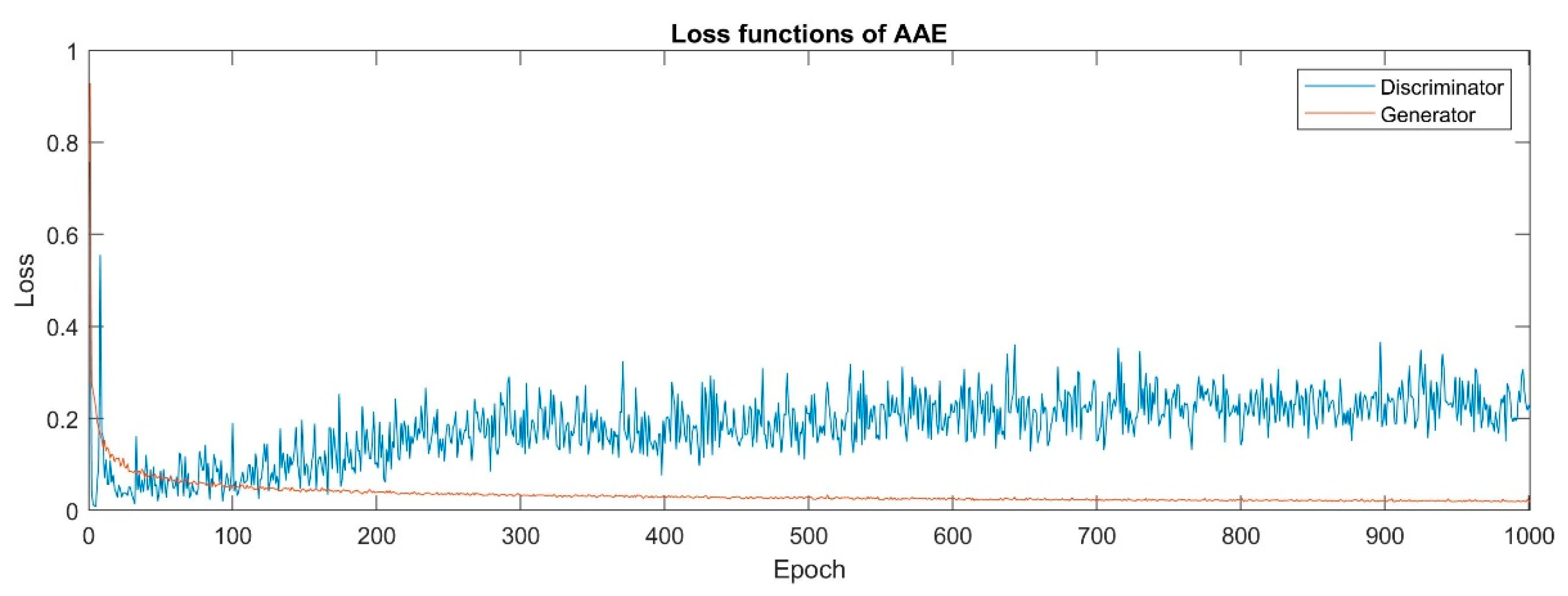
Taking the first dataset as an example, the training process of the loss functions for CAE, AAE, and SAE can be depicted, respectively, as shown in Figure 3, Figure 4 and Figure 5. The training processes of all loss functions slowly decline and show the convergence of the model parameters. Note that the deep structure of CAE is represented, as shown in Table 1.
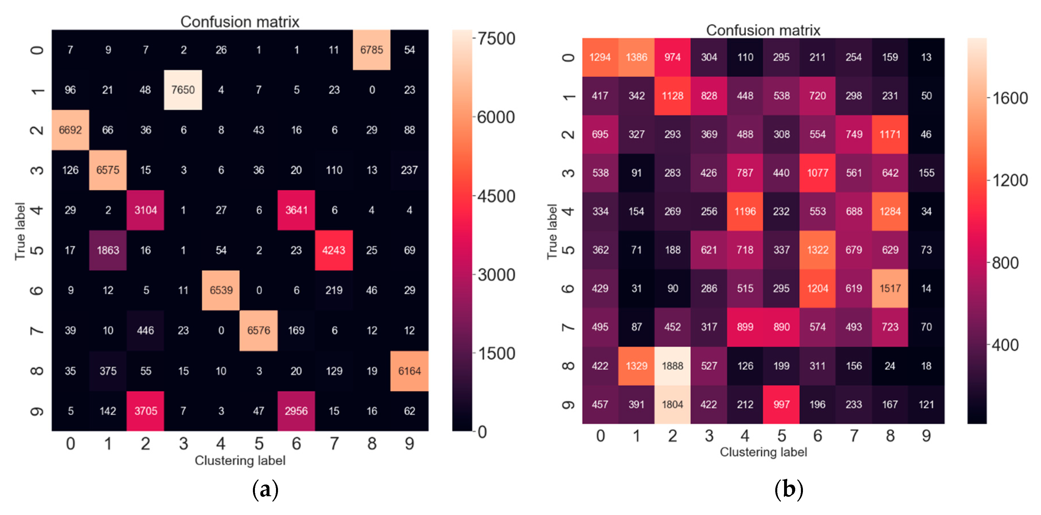
Then, we can use the representation code from SAE for image clustering by k-means. Taking Model 1 in the results of the MNIST and CIFAR-10 datasets as an example, we can obtain the confusion matrices between the ground-truth and predicted labels, respectively, as shown in Figure 6a,b. The performance comparison between the proposed methods and others can be presented, as shown in Table 2. Note that the best result of each clustering criterion is highlighted in bold and the results of other methods are extracted from [26], where FCM is the fuzzy objective function algorithm [27], SC is the spectral clustering algorithm [28], LRR is the low-rank representation algorithm [29], LSR1 and LSR2 are the variants of the least squares regression (LSR) [30], SLRR is the scalable LRR [31], LSC-R and LSC-K are the variants of the large-scale spectral clustering (LSC) algorithms [32], NMF is the non-negative matrix factorization algorithm [33], ZAC is the Zeta function based agglomerative clustering algorithm [34], and DEC is the deep embedding clustering algorithm [8].
The test process is described as follows. First, we use the BAE to extract the hidden codes. Then these codes are used in k-means to run the clustering algorithm. The initial centroids are determined randomly and the number of the clusters is predefined by the datasets, i.e., 10 clutters for each dataset. The distance between the centroids and the points is calculated by the Euclidean distance. Finally, we calculate the ACC, NMI, and ARI of each model in both datasets. Note that we run five times of the above test process and select the best solution.
The k-means algorithm is the most popular benchmark of the clustering methods. The result of Table 1 indicates that the k-means algorithm performs better than many algorithms. In addition, the empirical results indicate that the proposed models outperform others with respect to the criteria of ACC, NMI, and ARI in both datasets. The CIFAR-10 dataset is harder to recognize than the MNIST dataset; however, the proposed models can obtain better results than others. Even though the result of DEC also performs well, the result shows that the proposed models are more competitive. In addition, the DEC algorithm seems to have difficulty dealing with the CIFAR-10 dataset, since the criteria of the ACC, NMI, and ARI of DEC are worse than the benchmark; i.e., the k-means algorithm.

5. Discussion

Image clustering is an important issue in the fields of machine learning and computer vision. Traditional methods, such as k-means or the Wald method, cannot perform well due to their restricted capability with high-dimensional pixels. With the successful introduction of AE-based models such as SAE, CAE, and AAE, the clustering accuracy is dramatically increased. However, a single model may not have sufficient capability to extract all important feature representations from images, since each algorithm has its specialty for extracting a specific feature space. Hence, we consider a hybrid AE-based algorithm to extract a more complete feature space of images.
The characteristics of the proposed algorithm have the following advantages. First, we consider three distinct AE-based algorithms to extract the feature space as abundantly as possible. Second, the proposed algorithm considers the deep structure of the models to capture high-level feature representations. Furthermore, the proposed algorithm provides flexibility for further applications, such as classification or regression. For example, we can add a density layer behind the hidden code and use softmax or a linear function to consider the classification or the regression problem, respectively.
In addition, the results of the numerical experiments show that the proposed algorithm outperforms other methods with respect to the criteria of ACC, NMI, and ARI. Furthermore, although the proposed algorithm is combined with CAE and AAE, the performance of the proposed algorithms is better than that of CAE and AAE and justify the reason why we should consider a hybrid algorithm. However, the parameters of the model also significantly increase, and more time is needed to obtain convergent results. Future study may consider more different AE-based algorithms, such as the denoising autoencoder, sparse autoencoder, etc., to survey which combinations would be best for a specific dataset.

6. Conclusions

In this paper, we combine the characteristics of CAE, AAE, and SAE to form the proposed method, i.e., BAE, to handle the problem of image clustering. We use MNIST and CIFAR-10 datasets to test the proposed modes in the numerical experiment, and the results indicate that the proposed models are competitive with other methods. All clustering criteria, including ACC, NMI, and ARI criteria, are better than others. Further research could consider other hybrid models to combine the advantages of different models to get better results.

Author Contributions

Conceptualization, P.-Y.C. and J.-J.H.; methodology, J.-J.H.; software, J.-J.H.; validation, P.-Y.C.; writing—original draft preparation, P.-Y.C.; writing—review and editing, J.-J.H.

Funding

This research received no external funding.

Conflicts of Interest

The authors declare no conflict of interest.

References

  1. Fayyad, U.; Piatetsky-Shapiro, G.; Smyth, P. The KDD process for extracting useful knowledge from volumes of data. Commun. ACM 1996, 39, 27–34. [Google Scholar] [CrossRef]
  2. Chang, J.; Wang, L.; Meng, G.; Xiang, S.; Pan, C. Deep adaptive image clustering. In Proceedings of the IEEE Conference on Computer Vision and Pattern Recognition, Honolulu, HI, USA, 21–26 July 2017; pp. 5879–5887. [Google Scholar]
  3. Guo, X.; Liu, X.; Zhu, E.; Yin, J. Deep clustering with convolutional autoencoders. In Proceedings of the 24th International Conference on Neural Information Processing, Guangzhou, China, 14–17 November 2017; pp. 373–382. [Google Scholar]
  4. Alireza, M.; Shlens, J.; Jaitly, N.; Goodfellow, I.; Frey, B. Adversarial autoencoders. arXiv 2015, preprint. arXiv:1511.05644. [Google Scholar]
  5. Hinton, G.E.; Salakhutdinov, R.R. Reducing the Dimensionality of Data with Neural Networks. Science 2006, 313, 504–507. [Google Scholar] [CrossRef] [PubMed] [Green Version]
  6. Kingma, D.P.; Welling, M. Auto-encoding variational bayes. arXiv 2013, preprint. arXiv:1312.6114. [Google Scholar]
  7. Rezende, D.J.; Mohamed, S.; Wierstra, D. Stochastic backpropagation and approximate inference in deep generative models. Int. Conf. Mach. Learn. 2014, 32, 1278–1286. [Google Scholar]
  8. Xie, J.; Girshick, R.; Farhadi, A. Unsupervised deep embedding for clustering analysis. In Proceedings of the International Conference on Machine Learning, New York, NY, USA, 19–24 June 2016; pp. 478–487. [Google Scholar]
  9. Dilokthanakul, N.; Mediano, P.A.M.; Garnelo, M.; Lee, M.C.H.; Salimbeni, H.; Arulkumaran, K.; Shanahan, M. Deep Unsupervised Clustering with Gaussian Mixture Variational Autoencoders. arXiv 2016, arXiv:1611.02648. [Google Scholar]
  10. Liu, H.; Shao, M.; Li, S.; Fu, Y. Infinite ensemble for image clustering. In Proceedings of the 22nd ACM SIGKDD International Conference on Knowledge Discovery and Data Mining, San Francisco, CA, USA, 13–17 August 2016; pp. 1745–1754. [Google Scholar]
  11. Miguel, N.; McDermott, J. A hybrid autoencoder and density estimation model for anomaly detection. In International Conference on Parallel Problem Solving from Nature; Springer: Cham, Switzerland, 2016; pp. 717–726. [Google Scholar]
  12. Wang, C.; Pan, S.; Long, G.; Zhu, X.; Jiang, J. Mgae: Marginalized graph autoencoder for graph clustering. In Proceedings of the 2017 ACM on Conference on Information and Knowledge Management, Singapore, 6–10 November 2017; pp. 889–898. [Google Scholar]
  13. Sakurada, M.; Yairi, T. Anomaly detection using autoencoders with nonlinear dimensionality reduction. In Proceedings of the 2nd MLSDA Workshop on Machine Learning for Sensory Data Analysis, Gold Coast, Australia, 2 December 2014; p. 4. [Google Scholar]
  14. Wang, Y.; Yao, H.; Zhao, S. Auto-encoder based dimensionality reduction. Neurocomputing 2016, 184, 232–242. [Google Scholar] [CrossRef]
  15. Sun, W.; Shao, S.; Zhao, R.; Yan, R.; Zhang, X.; Chen, X. A sparse auto-encoder-based deep neural network approach for induction motor faults classification. Measurement 2016, 89, 171–178. [Google Scholar] [CrossRef]
  16. Bose, T.; Majumdar, A.; Chattopadhyay, T. Machine Load Estimation Via Stacked Autoencoder Regression. In Proceedings of the 2018 IEEE International Conference on Acoustics, Speech and Signal Processing (ICASSP), Calgary, AB, Canada, 15–20 April 2018; pp. 2126–2130. [Google Scholar]
  17. Dalal, N.; Triggs, B. Histograms of oriented gradients for human detection. In Computer Vision and Pattern Recognition 2005, Proceedings of the IEEE Computer Society Conference (CVPR 2005), San Diego, CA, USA, 20–25 June 2005; IEEE: New York, NY, USA, 2005; Volume 1, pp. 886–893. [Google Scholar]
  18. Lowe, D.G. Distinctive Image Features from Scale-Invariant Keypoints. Int. J. Comput. Vis. 2004, 60, 91–110. [Google Scholar] [CrossRef]
  19. Roy, M.; Bose, S.K.; Kar, B.; Gopalakrishnan, P.K.; Basu, A. A Stacked Autoencoder Neural Network based Automated Feature Extraction Method for Anomaly detection in On-line Condition Monitoring. In Proceedings of the 2018 IEEE Symposium Series on Computational Intelligence (SSCI), Bengaluru, India, 18–21 November 2018; pp. 1501–1507. [Google Scholar]
  20. Li, W.; Fu, H.; Yu, L.; Gong, P.; Feng, D.; Li, C.; Clinton, N. Stacked Autoencoder-based deep learning for remote-sensing image classification: a case study of African land-cover mapping. Int. J. Remote. Sens. 2016, 37, 5632–5646. [Google Scholar] [CrossRef]
  21. Ian, G.; Pouget-Abadie, J.; Mirza, M.; Xu, B.; Warde-Farley, D.; Ozair, S.; Courville, A.; Bengio, Y. Generative adversarial nets. In Advances in Neural Information Processing Systems 27, Proceedings of the Neural Information Processing Systems Conference (NIPS 2014), Montreal, QC, Canada, 8–13 December 2014; Curran Associates Inc.: Red Hook, NY, USA, 2014; pp. 2672–2680. [Google Scholar]
  22. Mukherjee, S.; Asnani, H.; Lin, E.; Kannan, S. ClusterGAN: Latent Space Clustering in Generative Adversarial Networks. arXiv 2018, preprint. arXiv:1809.03627. [Google Scholar]
  23. Chen, X.; Duan, Y.; Houthooft, R.; Schulman, J.; Sutskever, I.; Abbeel, P. InfoGAN: Interpretable Representation Learning by Information Maximizing Generative Adversarial Nets. In Advances in Neural Information Processing Systems 29, Proceedings of the 2016 Conference on Neural Information Processing Systems, Barcelona, Spain, 5–10 December 2016; Curran Associates Inc.: Red Hook, NY, USA, 2016; pp. 2172–2180. [Google Scholar]
  24. Vincent, P.; Larochelle, H.; Lajoie, I.; Bengio, Y.; Manzagol, P.A. Stacked denoising autoencoders: Learning useful representations in a deep network with a local denoising criterion. J. Mach. Learn. Res. 2010, 11, 3371–3408. [Google Scholar]
  25. Ralf, S.; Kurths, J.; Daub, C.O.; Weise, J.; Selbig, J. The mutual information: detecting and evaluating dependencies between variables. Bioinformatics 2002, 18 (Suppl. 2), S231–S240. [Google Scholar]
  26. Peng, X.; Zhou, J.T.; Zhu, H. k-meansNet: When k-means Meets Differentiable Programming. arXiv 2018, arXiv:1808.07292. [Google Scholar]
  27. Bezdek, J.C. Pattern Recognition with Fuzzy Objective Function Algorithms; Springer Science & Business Media: Berlin, Germany, 2013. [Google Scholar]
  28. Nie, F.; Zeng, Z.; Tsang, I.W.; Xu, D.; Zhang, C. Spectral Embedded Clustering: A Framework for In-Sample and Out-of-Sample Spectral Clustering. IEEE Trans. Neural Netw. 2011, 22, 1796–1808. [Google Scholar] [PubMed]
  29. Liu, G.; Lin, Z.; Yan, S.; Sun, J.; Yu, Y.; Ma, Y. Robust recovery of subspace structures by low-rank representation. IEEE Trans. Pattern Anal. Mach. Intell. 2012, 35, 171–184. [Google Scholar] [CrossRef] [PubMed]
  30. Lu, C.Y.; Min, H.; Zhao, Z.Q.; Zhu, L.; Huang, D.S.; Yan, S. Robust and efficient subspace segmentation via least squares regression. In Computer Vision—ECCV 2012, Proceedings of the European Conference on Computer Vision, Florence, Italy, 7–13 October 2012; Springer: Berlin/Heidelberg, Germany, 2012; pp. 347–360. [Google Scholar]
  31. You, C.; Li, C.-G.; Robinson, D.P.; Vidal, R. Oracle Based Active Set Algorithm for Scalable Elastic Net Subspace Clustering. In Proceedings of the 2016 IEEE Conference on Computer Vision and Pattern Recognition (CVPR), Las Vegas, NV, USA, 26 June–1 July 2016; pp. 3928–3937. [Google Scholar]
  32. Cai, D.; Chen, X. Large scale spectral clustering via landmark-based sparse representation. IEEE Trans. Cybern. 2014, 45, 1669–1680. [Google Scholar] [PubMed]
  33. Cai, D.; He, X.; Han, J. Locally consistent concept factorization for document clustering. IEEE Trans. Knowl. Data Eng. 2010, 23, 902–913. [Google Scholar] [CrossRef]
  34. Zhao, D.; Tang, X. Cyclizing clusters via zeta function of a graph. In Advances in Neural Information Processing Systems, Proceedings of the 23rd Annual Conference on Neural Information Processing Systems, Vancuver, BC, Canada, 7–10 December 2009; MIT Press: Cambridge, MA, USA, 2009; pp. 1953–1960. [Google Scholar]
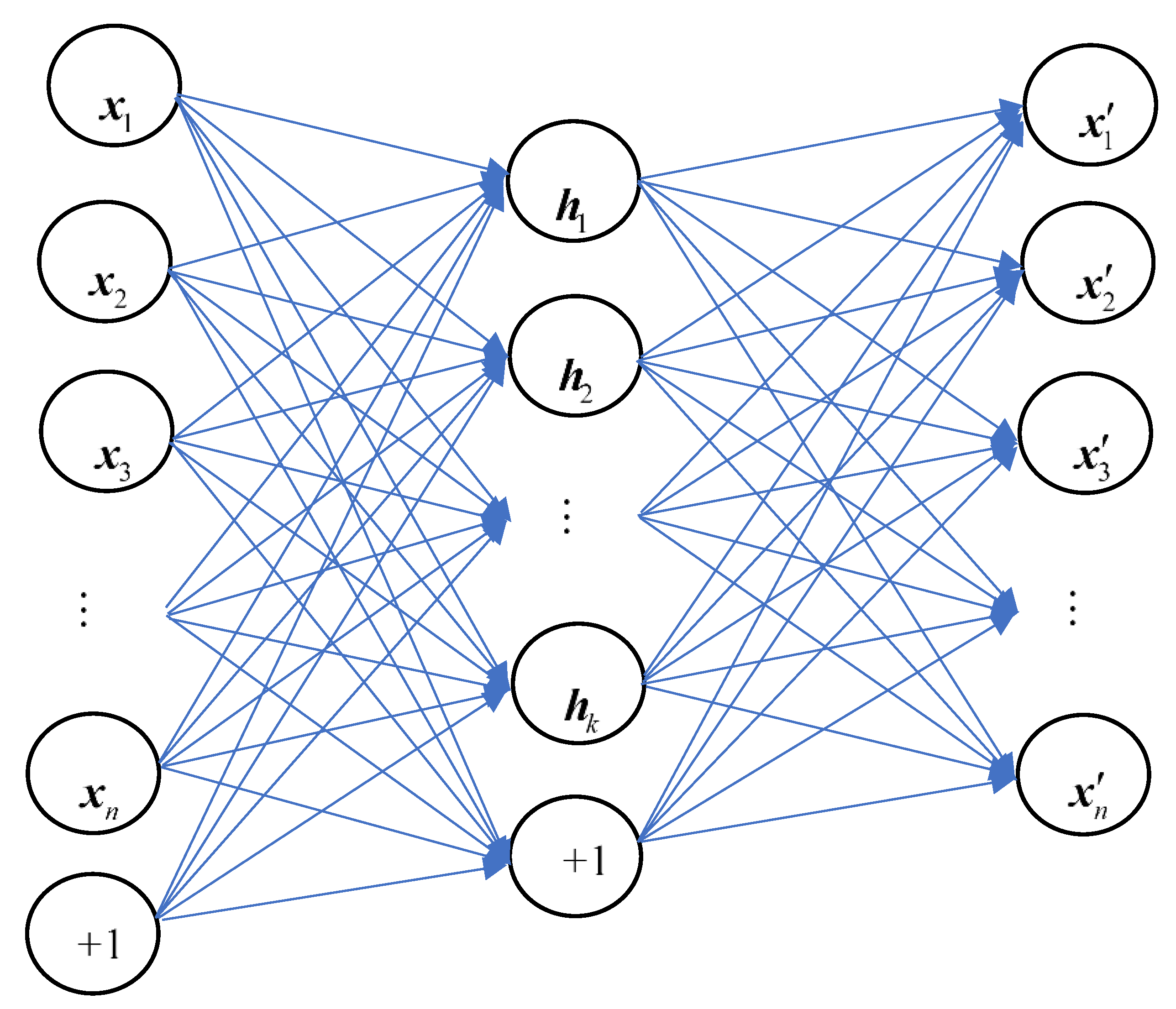
Figure 1. The structure of an autoencoder (AE).
Algorithms 12 00122 g001
Figure 2. Structure of the hybrid autoencoder. CAE: convolutional autoencoder; SAE: stacked autoencoder; and AAE: adversarial autencoder.
Algorithms 12 00122 g002
Figure 3. The training process of CAE.
Algorithms 12 00122 g003
Figure 4. The training process of AAE.
Algorithms 12 00122 g004
Figure 5. The training process of SAE.
Algorithms 12 00122 g005
Figure 6. (a) Confusion matrix of MNIST; (b) Confusion matrix of CIFAR-10.
Algorithms 12 00122 g006
Table 1. The deep structure of CAE.
LayerOutput ShapeNumber of Parameters
Conv2D(28,18,16)160
Maxpooling(14,14,16)0
Conv2D(14,14,2)290
Maxpooling(7,7,2)0
Conv2D(7,7,2)38
Upsampling(14,14,2)0
Conv2D(14,14,16)304
Upsampling(14,14,16)0
Conv2D(28,28,1)145
Table 2. The performance comparison between various clustering methods.
ModelsMNISTCIFAR-10
ACCNMIARIACCNMIARI
k-means0.78320.77750.70530.19810.05940.0301
FCM0.21560.12390.05100.17020.03920.0256
SC0.71280.73180.62180.19810.04720.0322
LRR0.21070.10430.10030.13070.04300.0030
LSR10.40420.31510.21350.19790.06050.0364
LSR20.41430.30030.20000.19080.06370.0316
SLRR0.21750.07570.55500.13090.01310.0094
LSC-R0.59640.56680.45980.18390.05670.0258
LSC-K0.72070.69880.60810.19290.06340.0389
NMF0.46350.43580.31200.19680.06200.0321
ZAC0.60000.65470.54070.05240.00360.0000
DEC 0.83650.73600.70100.18090.04560.0247
CAE0.68090.69630.56660.22320.08700.0451
AAE0.62170.59100.43510.13100.02040.0071
Hybrid Model 10.83670.80310.74900.23080.10020.0543
Hybrid Model 20.81040.80850.75800.22170.10170.0573
Unsupervised clustering accuracy: ACC, normalized mutual information: NMI, adjusted rand index: ARI.