Convolution Accelerator Designs Using Fast Algorithms


Abstract
1. Introduction
2. Related Works
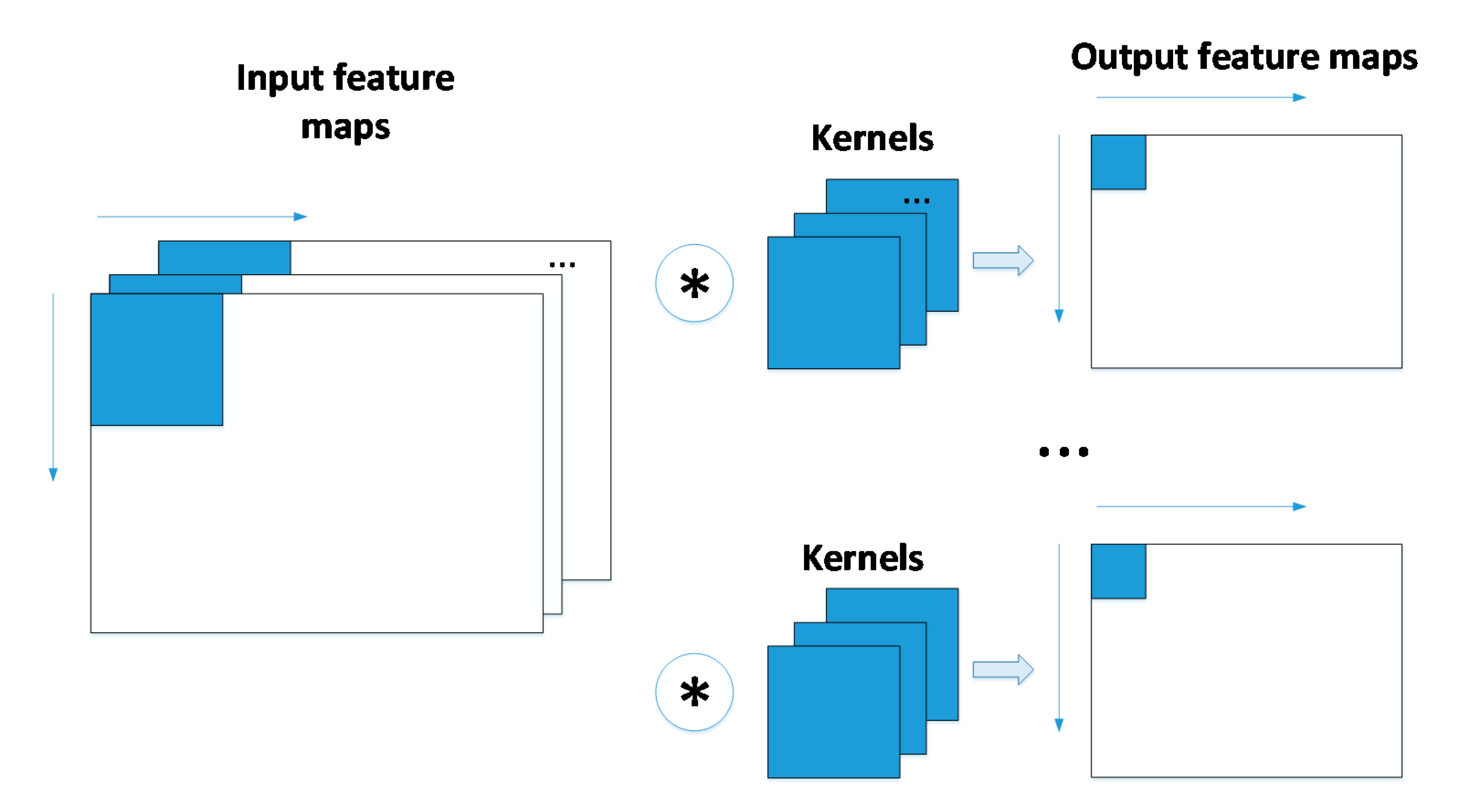
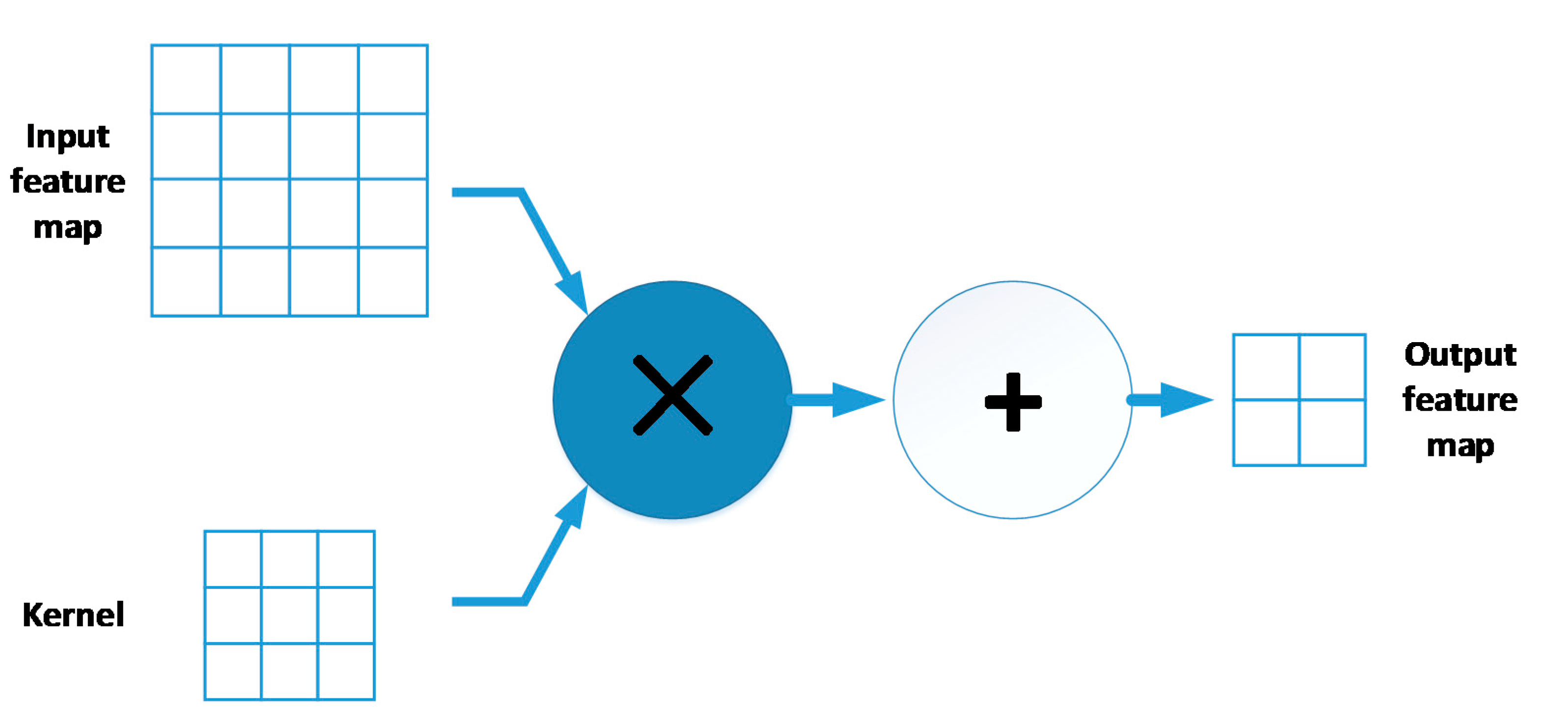
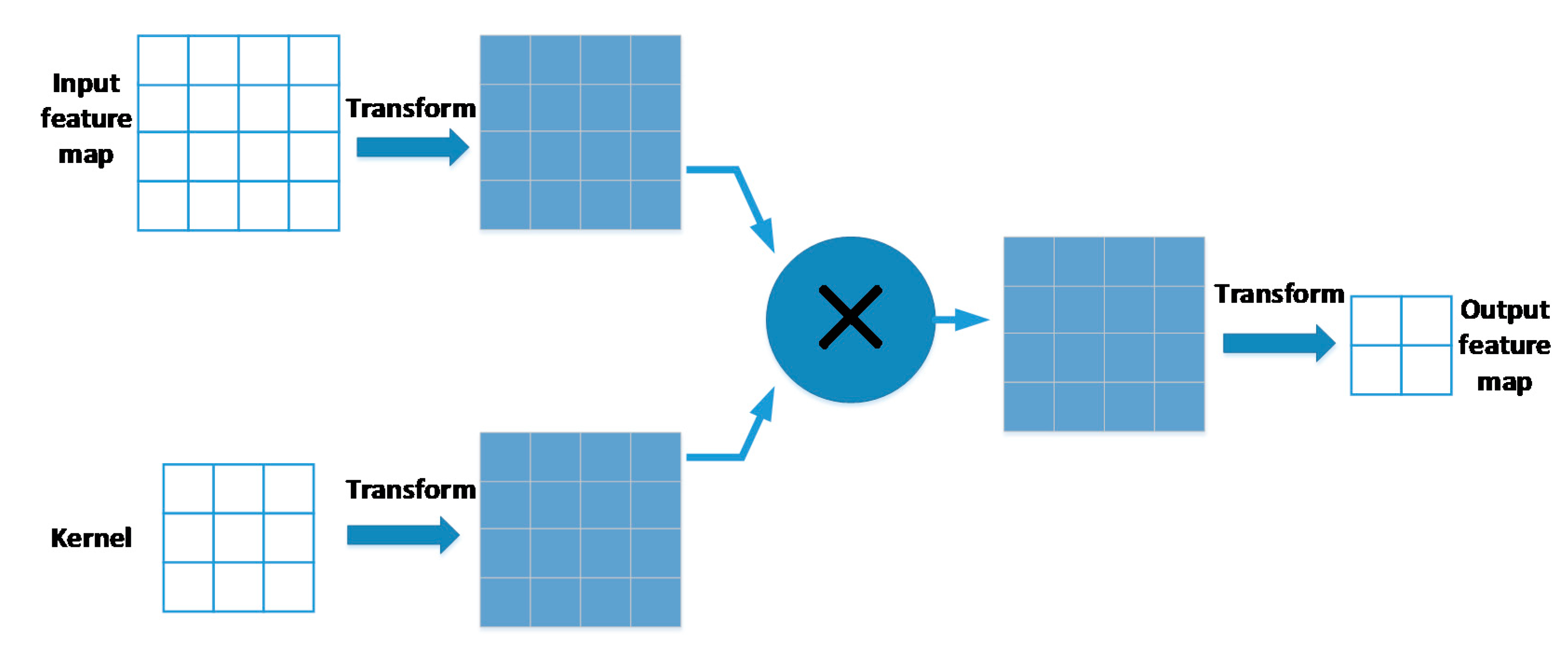
2.1. Convolutional Neural Network (CNN)
2.2. Strassen Algorithm
| Algorithm 1. Implementation of the Strassen Algorithm |
| 1 M1 = Conv(W1,1 + W2,2, X1,1 + X2,2) 2 M2 = Conv(W2,1 + W2,2, X1,1) 3 M3 = Conv(W1,1, X1,2 − X2,2) 4 M4 = Conv(W2,2, X2,1 − X1,1) 5 M5 = Conv(W1,1 + W2,2, X2,2) 6 M6 = Conv(W2,1 − W1,1, X1,1 + X1,2) 7 M7 = Conv(W1,2 − W2,2, X2,1 + X2,2) 8 Y1,1 = M1 + M4 − M5 + M7 9 Y1,2 = M3 + M5 10 Y2,1 = M2 + M4 11 Y2,2 = M1 − M2 + M3 + M6 |
2.3. Winograd Algorithm
2.4. Strassen–Winograd Algorithm
| Algorithm 2. Implementation of the Strassen–Winograd Algorithm |
| 1 M1 = Winograd(W1,1 + W2,2, X1,1 + X2,2) 2 M2 = Winograd(W2,1 + W2,2, X1,1) 3 M3 = Winograd(W1,1, X1,2 − X2,2) 4 M4 = Winograd(W2,2, X2,1 − X1,1) 5 M5 = Winograd(W1,1 + W2,2, X2,2) 6 M6 = Winograd(W2,1 − W1,1, X1,1 + X1,2) 7 M7 = Winograd(W1,2 − W2,2, X2,1 + X2,2) 8 Y1,1 = M1 + M4 − M5 + M7 9 Y1,2 = M3 + M5 10 Y2,1 = M2 + M4 11 Y2,2 = M1 − M2 + M3 + M6 |
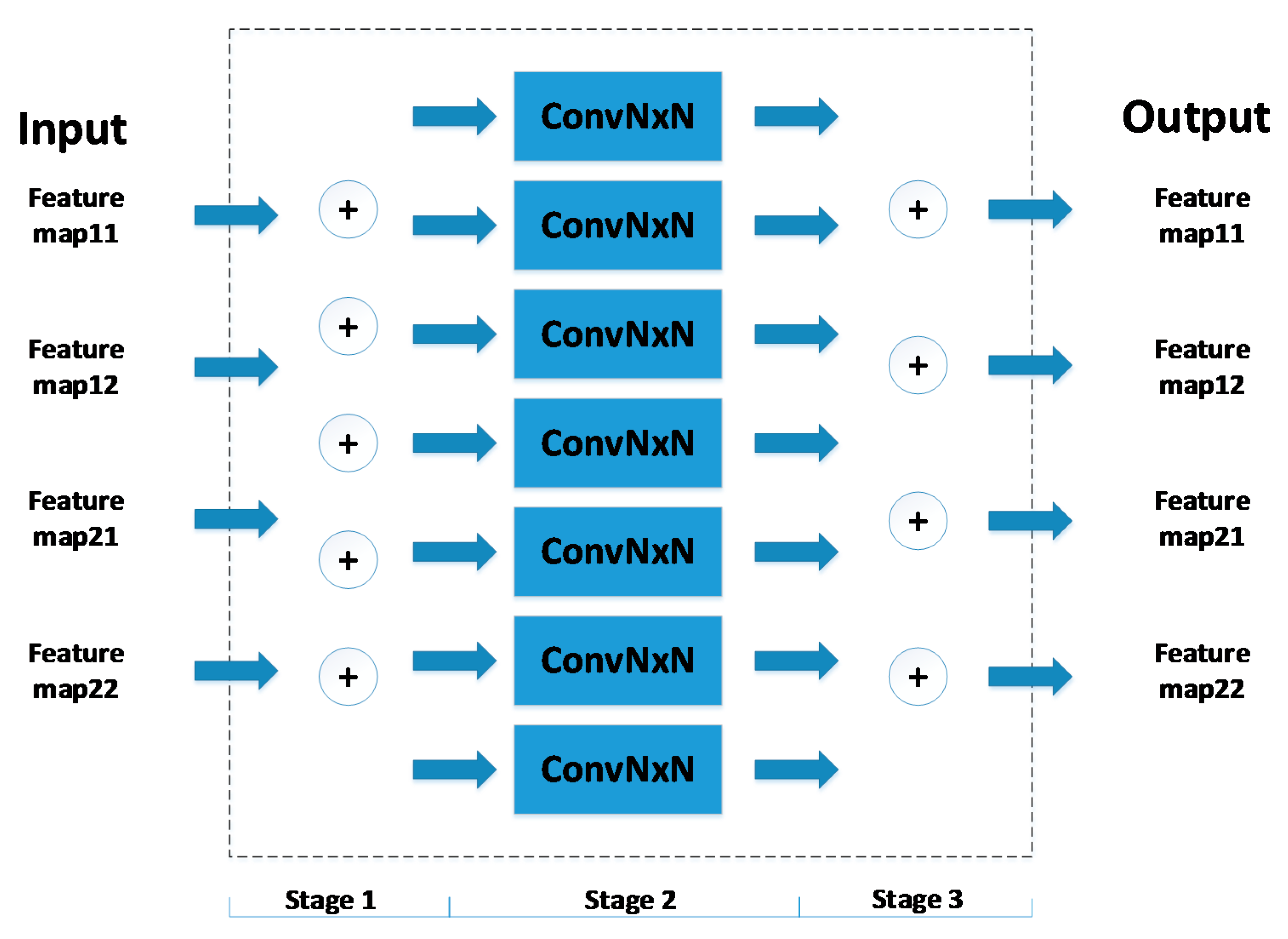
3. Architecture Design
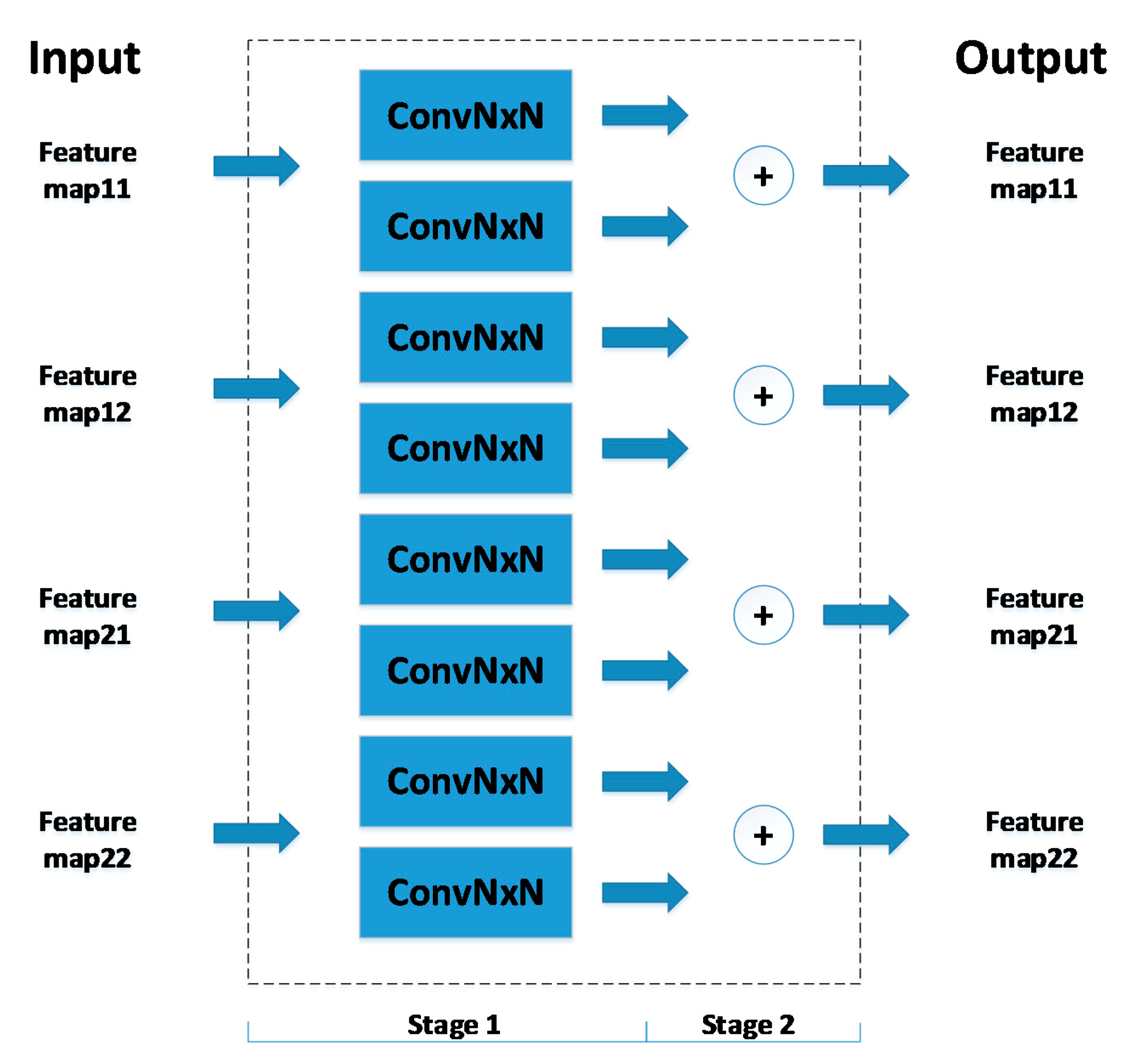
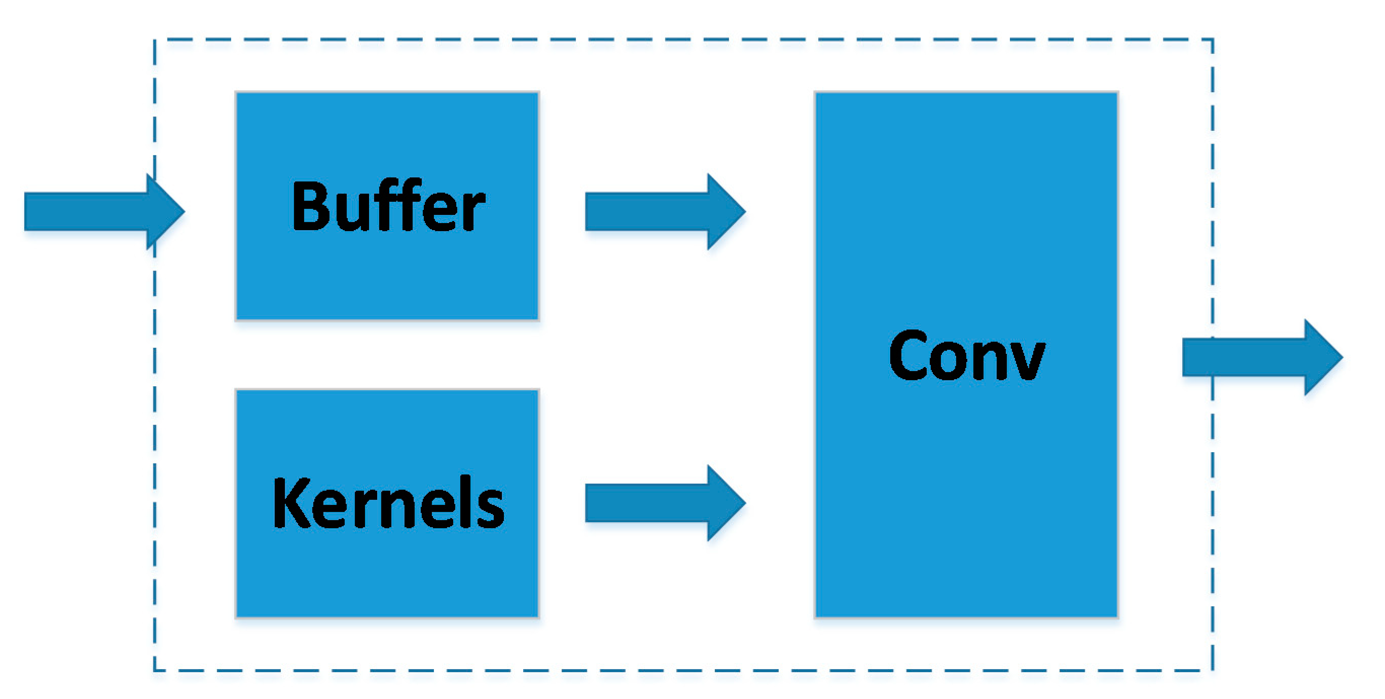
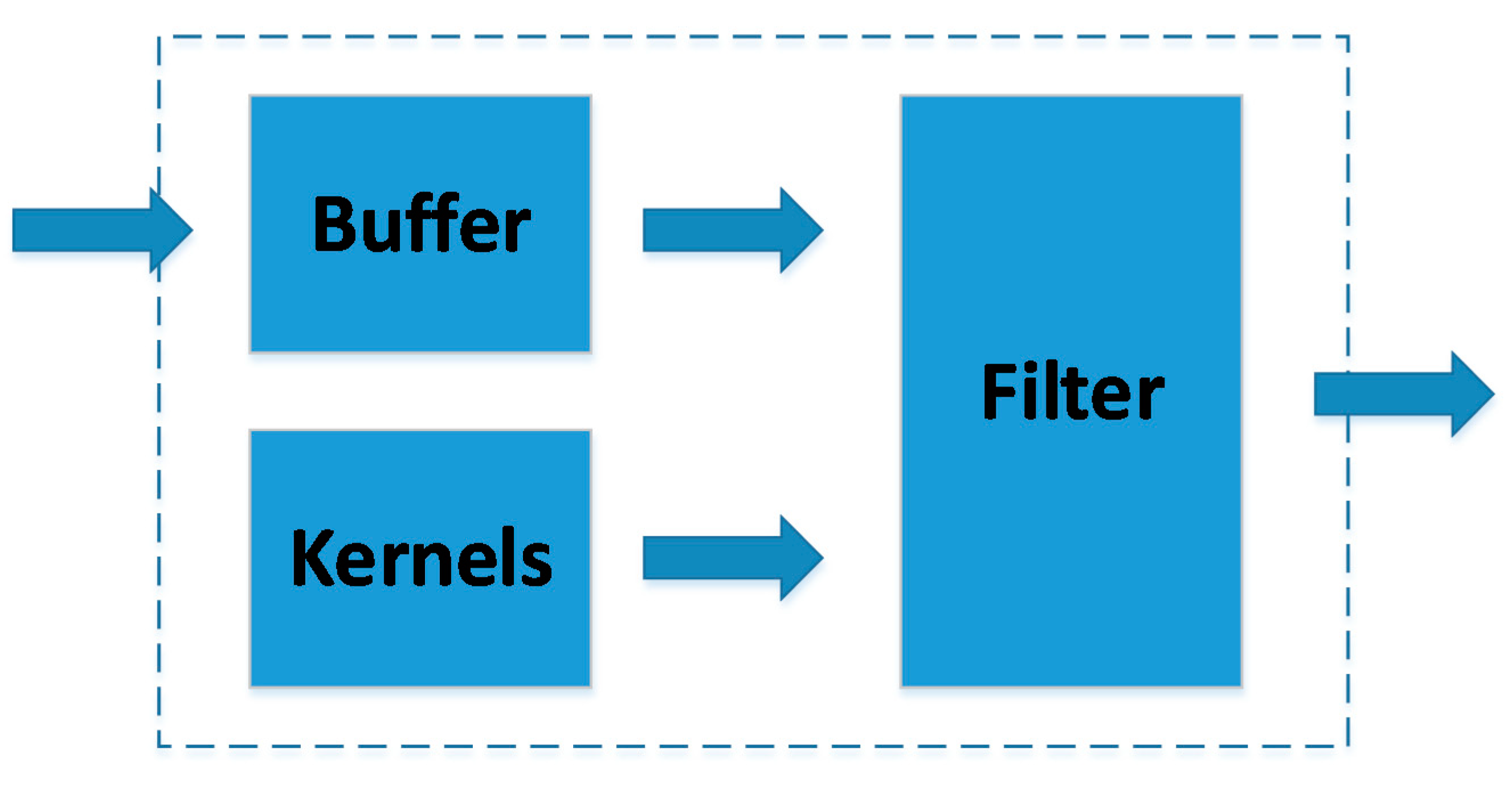
3.1. Conventional Design
3.2. Strassen Design
3.3. Winograd Design
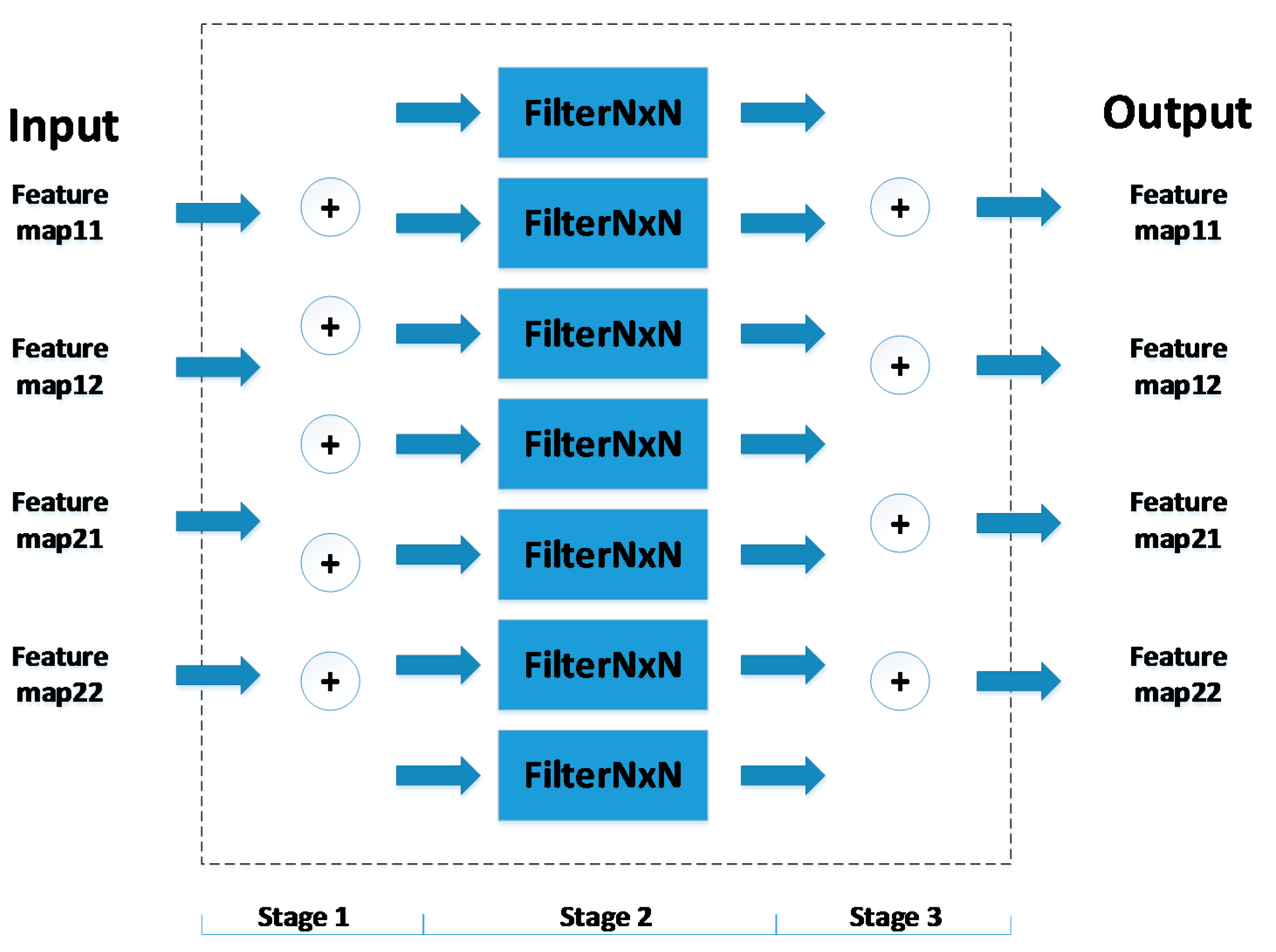
3.4. Strassen–Winograd Design
4. Implementation Results
5. Conclusions
Author Contributions
Funding
Conflicts of Interest
Appendix A
Appendix B
References
- Simonyan, K.; Zisserman, A. Very deep convolutional networks for large-scale image recognition. arXiv 2014. Available online: https://arxiv.org/pdf/1409.1556.pdf (accessed on 27 May 2019).
- Szegedy, C.; Liu, W.; Jia, Y. Going deeper with convolutions. arXiv 2014. Available online: https://arxiv.org/pdf/1409.4842.pdf (accessed on 27 May 2019).
- Liu, N.; Wan, L.; Zhang, Y.; Zhou, T.; Huo, H.; Fang, T. Exploiting Convolutional Neural Networks With Deeply Local Description For Remote Sensing Image Classification. IEEE Access 2018, 6, 11215–11228. [Google Scholar] [CrossRef]
- Krizhevsky, A.; Sutskever, I.; Hinton, G.E. ImageNet classification with deep convolutional neural networks. In Proceedings of the International Conference on Neural Information Processing Systems, Lake Tahoe, NV, USA, 3–6 December 2012; Volume 60, pp. 1097–1105. [Google Scholar]
- Le, N.M.; Granger, E.; Kiran, M. A comparison of CNN-based face and head detectors for real-time video surveillance applications. In Proceedings of the Seventh International Conference on Image Processing Theory, Tools and Applications, Montreal, QC, Canada, 28 November–1 December 2018. [Google Scholar]
- Ren, S.; He, K.; Girshick, R. Faster R-CNN: Towards real-time object detection with region proposal networks. In Proceedings of the International Conference on Neural Information Processing Systems, Montreal, QC, Canada, 8–13 December 2014; pp. 91–99. [Google Scholar]
- Denil, M.; Shakibi, B.; Dinh, L. Predicting Parameters in Deep Learning. In Proceedings of the International Conference on Neural Information Processing Systems, Lake Tahoe, NV, USA, 5–10 December 2013; pp. 2148–2156. [Google Scholar]
- Han, S.; Pool, J.; Tran, J. Learning Both Weights and Connections for Efficient Neural Networks. In Proceedings of the International Conference on Neural Information Processing Systems, Istanbul, Turkey, 9–12 November 2015; pp. 1135–1143. [Google Scholar]
- Guo, Y.; Yao, A.; Chen, Y. Dynamic Network Surgery for Efficient DNNs. In Advances in Neural Information Processing Systems; MIT Press: Cambridge, MA, USA, 2016; pp. 1379–1387. [Google Scholar]
- Colangelo, P.; Nasiri, N.; Nurvitadhi, E.; Mishra, A.; Margala, M.; Nealis, K. Exploration of Low Numeric Precision Deep Learning Inference Using Intel® FPGAs. In Proceedings of the IEEE 26th Annual International Symposium on Field-Programmable Custom Computing Machines, Boulder, CO, USA, 29 April–1 May 2018. [Google Scholar]
- Gupta, S.; Agrawal, A.; Gopalakrishnan, K.; Narayanan, P. Deep Learning with Limited Numerical Precision. In Proceedings of the International Conference on Machine Learning, Lille, France, 7–9 July 2015. [Google Scholar]
- Rastegari, M.; Ordonez, V.; Redmon, J. XNOR-Net: ImageNet Classification Using Binary Convolutional Neural Networks. In Proceedings of the European Conference on Computer Vision, Amsterdam, The Netherlands, 11–14 October 2016; Springer: Cham, Switzerland, 2016; pp. 525–542. [Google Scholar]
- Zhu, C.; Han, S.; Mao, H. Trained Ternary Quantization. In Proceedings of the International Conference on Learning Representations, Toulon, France, 24–26 April 2017. [Google Scholar]
- Vasilache, N.; Johnson, J.; Mathieu, M. Fast convolutional nets with fbfft: A GPU performance evaluation. In Proceedings of the International Conference on Learning Representations, San Diego, CA, USA, 7–9 May 2015. [Google Scholar]
- Qiu, J.; Wang, J.; Yao, S. Going Deeper with Embedded FPGA Platform for Convolutional Neural Network. In Proceedings of the 2016 ACM/SIGDA International Symposium on Field-Programmable Gate Arrays ACM, Monterey, CA, USA, 21–23 February 2016; pp. 26–35. [Google Scholar]
- Courbariaux, M.; Bengio, Y.; David, J. Training deep neural networks with low precision multiplications. arXiv 2015, arXiv:1412.7024. [Google Scholar]
- Hajduk, Z. High accuracy FPGA activation function implementation for neural networks. Neurocomputing 2017, 247, 59–61. [Google Scholar] [CrossRef]
- Bai, L.; Zhao, Y.; Huang, X. A CNN Accelerator on FPGA Using Depthwise Separable Convolution. IEEE Trans. Circuits Syst. II Express Briefs 2018, 65, 1415–1419. [Google Scholar] [CrossRef]
- Cong, J.; Xiao, B. Minimizing Computation in Convolutional Neural Networks. In Proceedings of the Artificial Neural Networks and Machine Learning—ICANN 2014, Hamburg, Germany, 15–19 September 2014. [Google Scholar]
- Lavin, A.; Gray, S. Fast Algorithms for Convolutional Neural Networks. In Proceedings of the Computer Vision and Pattern Recognition, Caesars Palace, NV, USA, 26 June–1 July 2016; pp. 4013–4021. [Google Scholar]
- Lu, L.; Liang, Y.; Xiao, Q.; Yan, S. Evaluating Fast Algorithms for Convolutional Neural Networks on FPGAs. In Proceedings of the IEEE 25th Annual International Symposium on Field-Programmable Custom Computing Machines, Napa, CA, USA, 30 April–2 June 2017; pp. 101–108. [Google Scholar]
- Zhao, Y.; Wang, D.; Wang, L.; Liu, P. A Faster Algorithm for Reducing the Computational Complexity of Convolutional Neural Networks. Algorithms 2018, 11, 159. [Google Scholar] [CrossRef]
- Coppersmith, D.; Winograd, S. Matrix multiplication via arithmetic progressions. J. Symb. Comput. 1990, 9, 251–280. [Google Scholar] [CrossRef]
- Lai, P.; Arafat, H.; Elango, V.; Sadayappan, P. Accelerating Strassen-Winograd’s matrix multiplication algorithm on GPUs. In Proceedings of the International Conference on High Performance Computing, data, and analytics, Karnataka, India, 18–21 December 2013. [Google Scholar]
- Strassen, V. Gaussian elimination is not optimal. Numer. Math. 1969, 13, 354–356. [Google Scholar] [CrossRef]
- Winograd, S. Arithmetic Complexity of Computations; SIAM: Philadelphia, PA, USA, 1980. [Google Scholar]


| Time Consumption | |
|---|---|
| Conventional | 125.48 µs |
| Strassen | 125.49 µs |
| Winograd | 125.49 µs |
| Strassen–Winograd | 125.50 µs |
| Slice Registers | Slice LUTs | Slices | DSP48E1s | |
|---|---|---|---|---|
| Available | 407,600 | 203,800 | 50,950 | 840 |
| Conventional | 5780 | 4635 | 2248 | 288 |
| Strassen | 5543 | 4642 | 2041 | 252 |
| Winograd | 9544 | 7752 | 3049 | 128 |
| Strassen–Winograd | 8751 | 7396 | 2713 | 112 |
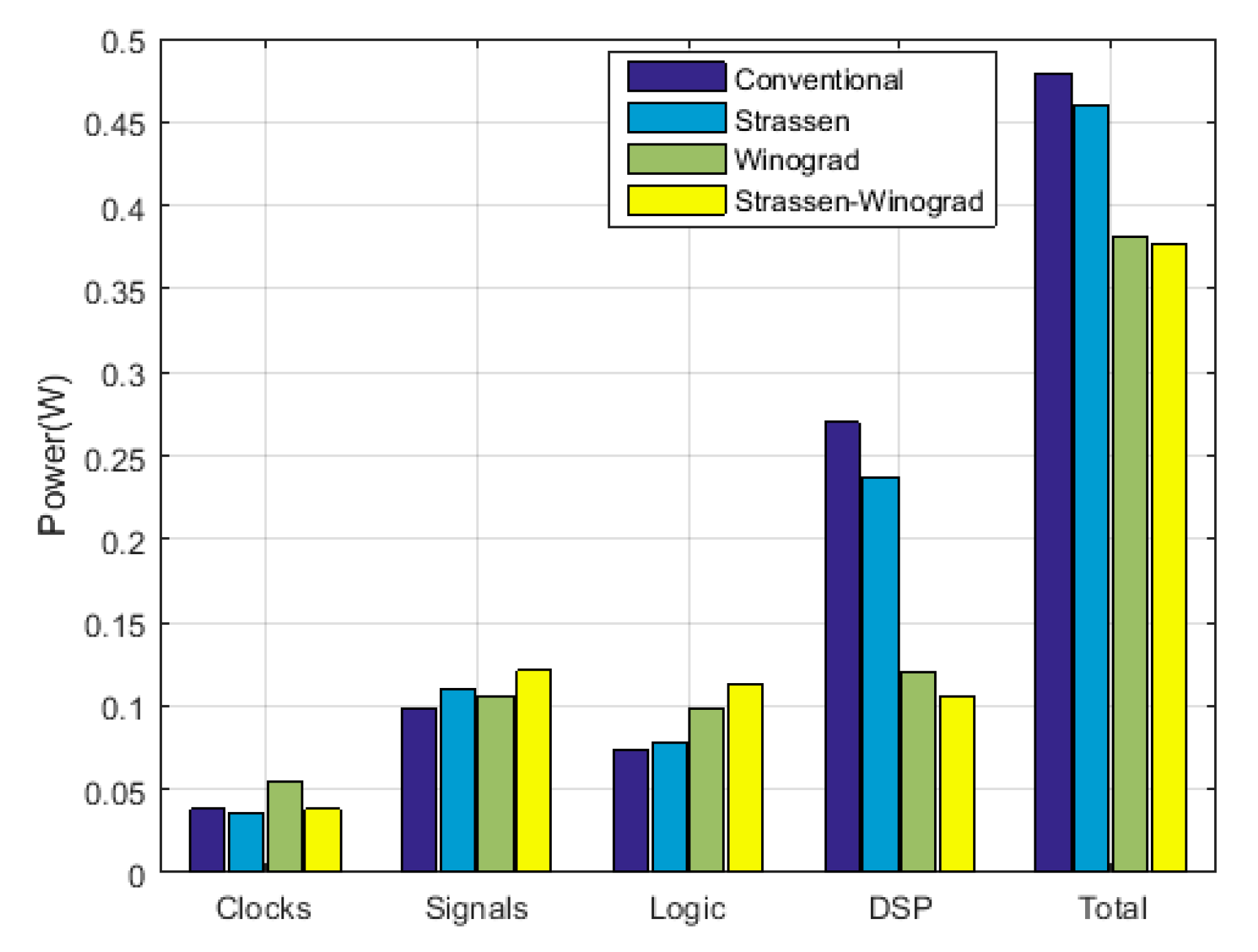
| Power (W) | Total | Clocks | Signals | Logic | DSP |
|---|---|---|---|---|---|
| Conventional | 0.479 | 0.038 | 0.098 | 0.073 | 0.270 |
| Strassen | 0.460 | 0.035 | 0.110 | 0.078 | 0.237 |
| Winograd | 0.381 | 0.055 | 0.106 | 0.099 | 0.120 |
| Strassen–Winograd | 0.377 | 0.038 | 0.121 | 0.113 | 0.105 |
© 2019 by the authors. Licensee MDPI, Basel, Switzerland. This article is an open access article distributed under the terms and conditions of the Creative Commons Attribution (CC BY) license (http://creativecommons.org/licenses/by/4.0/).
Share and Cite
Zhao, Y.; Wang, D.; Wang, L. Convolution Accelerator Designs Using Fast Algorithms. Algorithms 2019, 12, 112. https://doi.org/10.3390/a12050112
Zhao Y, Wang D, Wang L. Convolution Accelerator Designs Using Fast Algorithms. Algorithms. 2019; 12(5):112. https://doi.org/10.3390/a12050112
Chicago/Turabian StyleZhao, Yulin, Donghui Wang, and Leiou Wang. 2019. "Convolution Accelerator Designs Using Fast Algorithms" Algorithms 12, no. 5: 112. https://doi.org/10.3390/a12050112
APA StyleZhao, Y., Wang, D., & Wang, L. (2019). Convolution Accelerator Designs Using Fast Algorithms. Algorithms, 12(5), 112. https://doi.org/10.3390/a12050112