Improved Neural Networks Based on Mutual Information via Information Geometry

Abstract

This paper presents a new algorithm based on the theory of mutual information and information geometry. This algorithm places emphasis on adaptive mutual information estimation and maximum likelihood estimation. With the theory of information geometry, we adjust the mutual information along the geodesic line. Finally, we evaluate our proposal using empirical datasets that are dedicated for classification and regression. The results show that our algorithm contributes to a significant improvement over existing methods.

1. Introduction

An artificial neural network is a framework for many different machine learning algorithms to work together and process complex data inputs; it is vaguely inspired by biological neural networks that constitute animal brains [1]. Neural networks have been widely used in many application areas, such as systems identification [2], signal processing [3,4], and so on. Furthermore, several variants of neural networks have been derived from the context of applications. The convolutional neural network is one of the most popular variants. It is composed of one or more convolutional layers with fully connected layers and pooling layers [5]. In addition, the deep belief network (DBN) is considered to be a composition of simple learning modules that make up each layer [6]. Several restricted Boltzmann machines [7] are stacked and trained greedily to form the DBN. In 2013, Grossberg proposed a recurrent neural network, which is a class of artificial neural network in which connections between nodes form a directed graph along a sequence [8]. The output layer can obtain information from past and future states simultaneously.

However, improving the performance of a neural network remains an open question. From the viewpoint of information theory, mutual information is used to optimize neural networks. In the method of the ensemble, two neural networks are forced to convey different information about some features of their input by minimizing the mutual information between the variables extracted by the two neural networks [9]. In this method, mutual information is used to measure the correlation between two hidden neurons. In 2010, an adaptive merging and splitting algorithm (AMSA) pruned hidden neurons by merging correlated hidden neurons and added hidden neurons by splitting existing hidden neurons [10]. In this method, the mutual information is used to measure the correlation between the two hidden neurons. In 2015, Berglund et al. proposed measuring the usefulness of hidden units in Boltzmann machines with mutual information [11]. However, the measure is not suitable as the sole criterion for model selection. In addition, the measure that was shown to correlate well with the entropy does not agree with the well-known and observed phenomenon that sparse features that have in general low entropy are good for many machine learning tasks, including classification. By a new objective function, a neural network with maximum mutual information training is proposed to solve the problem of two-class classification [12]. It focuses on maximizing the difference between the estimated possibility of the two classes. However, when the two classes are completely separable, the algorithm cannot outperform the traditional algorithm of maximum likelihood estimation. To address the problems above, we introduce the theory of information geometry into neural networks.

Information geometry is a branch of mathematics that applies the theory of Riemannian manifolds to the field of probability theory [13]. By the Fisher information [14], the probability distributions for a statistical model are treated as the points of a Riemannian manifold. This approach focuses on studying the geometrical structures of parameter spaces of distributions. Information geometry has found various applications in many fields, such as control theory [15], signal processing [16], the expectation–maximization algorithm [17], and many others [18,19]. In addition, information geometry is used to study neural networks. In 1991, Amari [20] studied the dualistic geometry of the manifold of higher-order neurons. Furthermore, the natural gradient works efficiently in the learning of neural networks [21]. The natural gradient learning method can overcome some disadvantages in the learning process of the networks effectively, such as the slow learning speed and the existence of plateaus. In 2005, a novel information geometric-based variable selection criterion for multilayer perceptron networks was described [22]. It is based on projections of the Riemannian manifold as defined by a multilayer perceptron network on submanifolds with reduced input dimension.

In this paper, we propose a new algorithm based on the theory of mutual information and information geometry. We study the information covered by a whole neural network quantitatively via mutual information. In the proposed method, the learning of the neural network attempts to keep as much information as possible while maximizing the likelihood. Then, with the theory of information geometry, the optimization of the mutual information turns into minimizing the difference information between the estimated distribution and the original distribution. The distributions are mapping to points on a manifold. The Fisher distance is a proper measurement of the path between the points. Then, we obtain a unique solution of the mutual information by minimizing the Fisher distance between the estimated distribution and the original distribution along the shortest path (geodesic line).

2. Materials and Methods

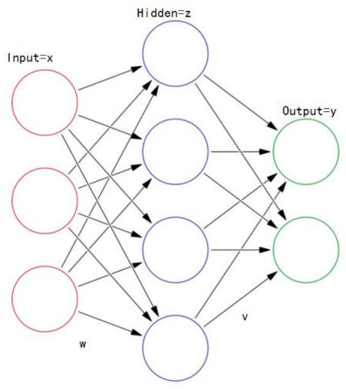
Let us consider a neural network with one input layer, one output layer, and one hidden layer. The weights for the input are denoted by $w$. The weights for the hidden neurons are $v$. Here, $x$ is the input, while $\tilde{y}$ is the actual output, and z is the activation of the hidden neurons. The concatenation of the output and hidden neurons is represented as a vector $r=[\tilde{y},z]$. Figure 1 illustrates the architecture of the neural network.

Figure 1. The architecture of the neural network.

The neural network is a static and usually nonlinear model

$$p(r|x)=p(\tilde{y},z|x,u)=p(\tilde{y}|z,v)p(z|x,w)$$

(1)

where the parameters of the neural network are denoted by $u=[w,v]$.

The mutual information (MI) [23] of two random variables quantifies the “amount of information” obtained about one random variable, through the other random variable. In the proposed algorithm, we treat the input $x$ and the combination of the output and hidden neurons $r$ as two random variables. Correspondingly, the MI quantifies the “amount of information” obtained by the output and hidden variable from the input. The learning of the neural network attempts to keep as much information as possible while maximizing the likelihood. We define a novel objective function as

$$J=E_x[{(\tilde{y}-y)}^2]+\lambda I(x;r)$$

(2)

where y is the desired output (i.e., the true value of the label). The first item is the objective function of traditional backpropagation neural networks, while the second item is the MI of $x$ and $r$. With the first item, we maximize the likelihood similar to what traditional neural networks do. With the second item, the proposed method helps the neural networks to keep information from the input. Here, $\lambda$ is a constant determined by experience.

Many methods exist for minimizing the first item, such as conjugate gradient [24]. Therefore, we just discuss how to work with the second item in this paper. By the definition of MI and Kullback–Leibler divergence (KLD) [25], the mutual information of x and $r$ is

$$\begin{array}{ll}I(x;r)& ={\displaystyle \underset{x\in X}{\int }{\displaystyle \underset{r\in R}{\int }p(x,r)\log \frac{p(x,r)}{p(x)p(r)}drdx}}\\ & ={\displaystyle \underset{x\in X}{\int }p(x)}{\displaystyle \underset{r\in R}{\int }p(r|x)\log }\frac{p(x,r)}{p(x)p(r)}drdx\\ & ={\displaystyle \underset{x\in X}{\int }p(x)}{\displaystyle \underset{r\in R}{\int }p(r|x)\log }\frac{p(r|x)}{p(r)}drdx\\ & ={\displaystyle \underset{x\in X}{\int }p(x)}KLD(p(r|x)||p(r))dx\end{array}$$

(3)

where $X$ is the value domain of x, while $R$ is the value domain of $r$.

In general, the density $p(x)$ is assumed to be unknown. Therefore, we make a finite-sample approximation, since we work with a finite dataset. The size of the set is N. Then, the mutual information in (3) is calculated as

$$I(x;r)=\frac{1}{N}\sum _{i=1}^{N}KLD(p(r|x_i)||p(r))$$

(4)

where $x_i$ is the $i$th input data.

In addition, we have

$$\begin{array}{ll}KLD(p(r|x_i)||p(r))& ={\displaystyle \underset{\tilde{y}\in Y,z\in Z}{\iint }p(\tilde{y}|z,v)p(z|x_i,w)\log \frac{p(\tilde{y}|z,v)p(z|x_i,w)}{p(\tilde{y}|z)p(z)}}d\tilde{y}dz\\ & ={\displaystyle \underset{z\in Z}{\int }p(z|x_i,w)}\log \frac{p(z|x_i,w)}{p(z)}\left({\displaystyle \underset{\tilde{y}\in Y}{\int }p(\tilde{y}|z,v)}d\tilde{y}\right)dz+{\displaystyle \underset{\tilde{y}\in Y,z\in Z}{\iint }p(\tilde{y}|z,v)p(z|x_i,w)\log \frac{p(\tilde{y}|z,v)}{p(\tilde{y}|z)}}d\tilde{y}dz\\ & ={\displaystyle \underset{z\in Z}{\int }p(z|x_i,w)}\log \frac{p(z|x_i,w)}{p(z)}dz+E_z\left[{\displaystyle \underset{\tilde{y}\in Y}{\int }p(\tilde{y}|z,v)\log \frac{p(\tilde{y}|z,v)}{p(\tilde{y}|z)}d\tilde{y}}\right]\\ & =KLD(p(z|x_i,w)||p(z))+E_z\left[KLD(p(\tilde{y}|z,v)||p(\tilde{y}|z))\right]\\ & =KLD(p(z|x_i,w)||p(z))+\frac{1}{N}{\displaystyle \sum _{i=1}^N}KLD(p(\tilde{y}|z_i,v)||p(\tilde{y}|z_i))\\ & =KLD(p(z|x_i,w)||p(z))\end{array}$$

(5)

where $z_i$ is the value of the vector of hidden neurons when the input is $x_i$, while $Z$ is the value domain of $z$, and $p(\tilde{y}|z_i,v)=p(\tilde{y}|z_i)$ so that $KLD(p(\tilde{y}|z_i,v)||p(\tilde{y}|z_i))=0$.

The original distribution $p(z)$ can be derived from a finite-sample approximation, which gives us the following:

$$p(z)=\frac{1}{N}\left[p(z|x_1,w)+p(z|x_2,w)+\dots +p(z|x_N,w)\right]=\frac{1}{N}\sum _{i=1}^{N}p(z|x_i,w)$$

(6)

Next, we will show an effective way to calculate the $KLD$ in (5) with the theory of information geometry.

Any function that can be written in the following form is from the exponential family [26]:

$$p(x|\theta )=\exp (x·\theta -\varphi (\theta ))$$

(7)

where $\varphi$ is a function of $\theta$.

Without loss of generality, the probability of the activation of each hidden unit can be approximated with a function from the exponential family [27]. Here, $z^j$ represents the $j$th hidden unit; then,

$$p(z^j|x_i,w)=p(z^j|{\theta }^j)=\exp (z^j·{\theta }^j-{\varphi }^j({\theta }^j))$$

(8)

where ${\theta }^j$ is a function of $x·w^j$ (i.e., the linear weighted input of $z^j$), while $w_j$ is the $j$th column of $w$, for $j\in \{1,2,\dots ,l\}$, and $l$ is the size of the hidden layer. Additionally, ${\varphi }^j$ is a function of ${\theta }^j$. Considering that the activations of the hidden neurons are independent, the probability of $z$ is calculated as

$$p(z|x_i,w)=p(z|\theta )=\prod _{j=1}^{l}p(z^j|{\theta }^j)=\prod _{j=1}^l\exp (z^j·{\theta }^j-{\varphi }^j({\theta }^j))=\exp (\sum _{j=1}^l{z}^j·{\theta }^j-\sum _{j=1}^l{\varphi }^j({\theta }^j))=\exp (z·\theta -\varphi (\theta ))$$

(9)

Thus, $p(z|\theta )$ is from the exponential family, while $\theta$ is a function of the linear input $x·w$ of $z$. In addition, $\varphi$ is a function of $\theta$.

A classic parametric space for this family of probability density functions (PDFs) is

$$H=\{\eta =\frac{\partial \varphi (\theta )}{\partial \theta }\}$$

(10)

For the distributions in the exponential family, there are two dual coordinate systems $\theta$ and $\eta$ on the manifold (which is defined as a topological space that locally resembles Euclidean space near each point) of the parameters [28]. Here, $\eta$ is given by

$$\eta =\frac{\partial \varphi (\theta )}{\partial \theta }=E(z)$$

(11)

With (9) and (11), we calculate the ${\eta }_i$ for each $z_i$. From (6), it is evident that the $p(z)$ is the mean of the conditional probability over each input $x_i$. Thus, with (11), the parameters in the density in (6) are approximated by

$$\overline{\eta }=\frac{1}{N}\sum _{i=1}^N{\eta }_i$$

(12)

For the distribution in the exponential family, we have

$$\psi (\eta )={\displaystyle \int p(z|\eta )}\log p(z|\eta )dr$$

(13)

For distribution with $n$ parameters, the Fisher distance between two points ${\theta }^{\prime }$ and $\theta *$ in the half-plane $H$ reflects the dissimilarity between the associated PDF’s. It is defined as the minimal integral [29]

$$d_F({\theta }^{\prime },\theta *):=\underset{\theta (t)}{\min }{\displaystyle {\int }_{{\theta }^{\prime }}^{\theta *}(\sqrt{{(\frac{d\theta }{dt})}^{T}G(\theta )(\frac{d\theta }{dt})})}dt$$

(14)

where $\theta (t)$ represents a curve that is parameterized by $t$, while $G(\theta )$ is the Fisher information matrix which is defined as

$$G(\theta )=[g_{ab}(\theta )]$$

(15)

$$g_{ab}(\theta )=E\left[\frac{\partial \log p(z|\theta )}{\partial {\theta }_a}\frac{\partial \log p(z|\theta )}{\partial {\theta }_b}\right]$$

(16)

where $a\in \{1,2,\dots ,n\}$ and $b\in \{1,2,\dots ,n\}$ are the indexes of the elements in $G$.

The curve that satisfies the minimization condition in (14) is called a geodesic line.

Theorem 1

[30]. For the distributions in the exponential family, the Fisher distance is the Kullback–Leibler divergence given by

$$KLD(p(z|{\theta }^{\prime })||p(z|\eta *))=\varphi ({\theta }^{\prime })+\psi (\eta *)-{\theta }^{\prime }·\eta *$$

(17)

With (11) to (13), we obtain a dual description for $p(z)$, as follows:

$$\overline{\eta }=\nabla \varphi (\theta )$$

(18)

$$\psi (\overline{\eta })={\displaystyle \int p(z|\overline{\eta })}\log p(z|\overline{\eta })dr$$

(19)

Let ${\theta }^{\prime }=\theta$ and $\eta *=\overline{\eta }$ in (14). With (5), we have

$$KLD(p(r||x_i)||p(r))=KLD(p(z|\theta )||p(z))=\varphi (\theta )+\psi (\overline{\eta })-\theta ·\overline{\eta }$$

(20)

Then, we substitute (20) into (3) to obtain the second item in (2). By the definition of the Fisher distance (14) and Theorem 1, we know that minimizing the second item in (2) is equivalent to minimizing the Fisher distance between the estimated distribution $p(r|x_i)$ and the original distribution $p(r)$ along the shortest path (geodesic line). To describe the geodesic line using local coordinates, we must solve the geodesic equations given by the Euler–Lagrange equations, as follows:

$$\frac{d^2{\theta }_k}{d{t}^2}+{\displaystyle \sum _{a=1}^n{\displaystyle \sum _{b=1}^n(\frac{1}{2}{\displaystyle \sum _{a=1}^n{g}^{kl}(\frac{\partial g_{al}}{\partial {\theta }_b}+\frac{\partial g_{bl}}{\partial {\theta }_a}-\frac{\partial g_{ab}}{\partial {\theta }_l})})\frac{d{\theta }_a}{dt}}}\frac{d{\theta }_b}{dt}=0,\forall a,b,k,l\in \{1,\dots ,n\}$$

(21)

where $\theta ={({\theta }_1,{\theta }_2,\dots ,{\theta }_n)}^{\prime }$. By solving (21), one obtains a unique solution for the mutual information by minimizing the Fisher distance along the shortest path (geodesic line). In practice, we replace this step by the neural gradient descent [31], which makes the parameters in the second item in (2) update along the geodesic line. Here, the direction of the updating of the parameters is

$$\widehat{\nabla }\theta =G^{-1}(\theta )\nabla I(x;r)$$

(22)

where $\nabla$ is the common gradient.

3. Results

The proposed algorithm is used to improve a shallow neural network (NN) and a DBN [31]. The architectures of the networks are determined by the method in [32]. We use three popular datasets, namely, Iris, Poker Hand, and Forest Fires, from the UCI Machine Learning Repository (http://archive.ics.uci.edu/ml/datasets. html). With these datasets, we design several experiments to solve typical problems in machine learning, such as problems that involve classification and regression.

3.1. Classification

In machine learning, classification is the problem of classifying instances into one of two or more classes. For this issue, accuracy is defined as the accuracy rate of the classification.

We designed neural networks as classifiers to solve the classification problems from two datasets, Iris and Poker Hand. For each of these datasets, 50% of the training samples are used for learning. In these samples, the percent of labeled training samples $\alpha$ samples ranges from 10% to 50%. In the remainder of the dataset, 10% of the samples are randomly selected as test data. The constant $\lambda$ is set to −0.1.

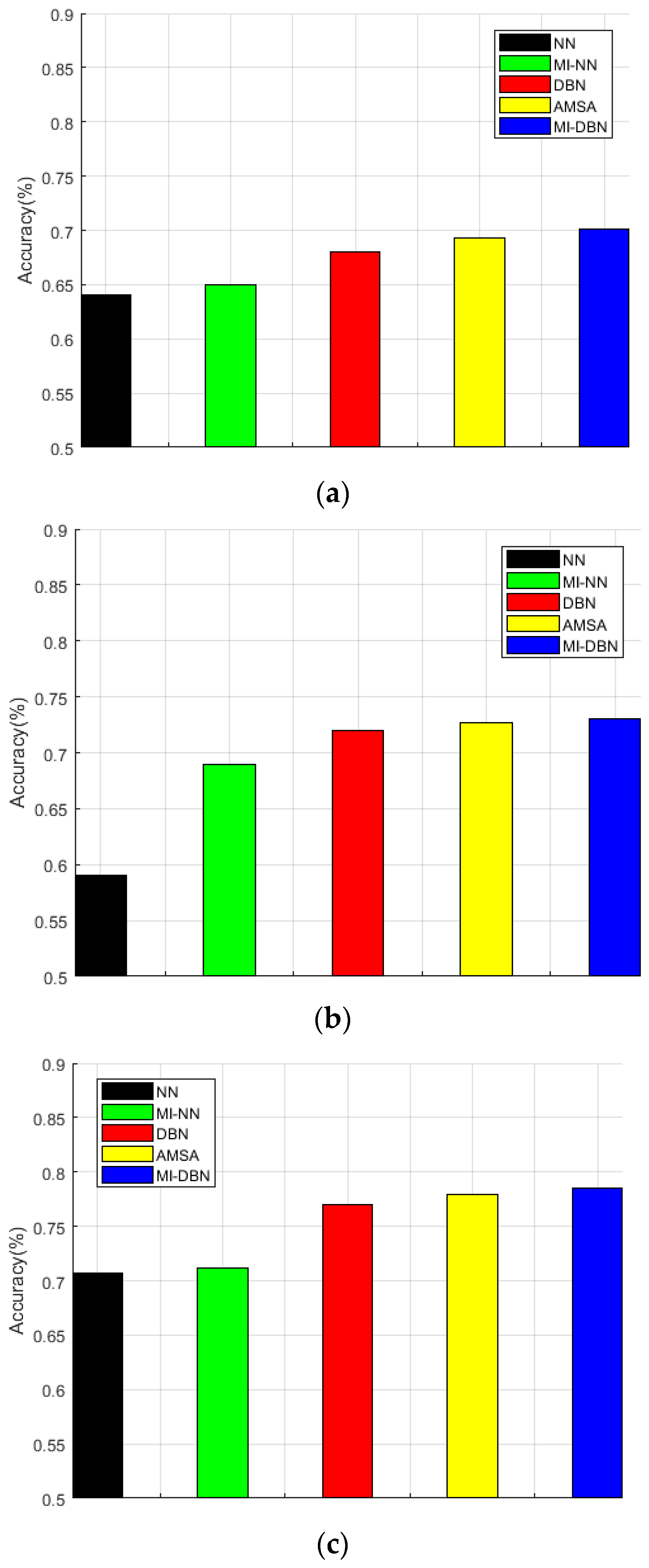
The test accuracy on the Iris dataset for NN, DBN, AMSA, MI-NN, and MI-DBN (“MI-“ denotes the proposed methods) can be seen in Figure 2. The network structures used in this experiment are 4-3-3 and 4-6-7-3, which correspond to the shallow networks (i.e., NN and MI-NN) and the deep networks (i.e., DBN, AMSA, and MI-DBN), respectively. The activation and output function is sigmoid.

Figure 2. The tests of NN, MI-NN, DBN, AMSA, and MI-DBN with Iris. The accuracies are plotted on the horizontal axis. (a) $\alpha =10\%$; (b) $\alpha =30\%$; (c) $\alpha =50\%$.

The test accuracies on the Poker Hand dataset for NN, DBN, AMSA, MI-NN, and MI-DBN (“MI-“ denotes the proposed methods) can be seen in Figure 3. The network structures used in this experiment are 85-47-10 and 85-67-48-10, which correspond to the shallow networks (i.e., NN and MI-NN) and the other networks (i.e., DBN, AMSA, and MI-DBN), respectively. The activation and output function is sigmoid.

Figure 3. The tests of NN, MI-NN, DBN, AMSA, and MI-DBN with Poker Hand. The accuracies are plotted on the horizontal axis. (a) $\alpha =10\%$; (b) $\alpha =30\%$; (c) $\alpha =50\%$.

It can be seen that the proposed algorithm outperforms the previous methods on both datasets successfully, although a sole exception is that the MI-NN is slightly worse than AMSA with Iris when $\alpha =10\%$. This finding means that the proposed algorithm can be applied to the problem of classification. In addition, the proposed algorithm improves the traditional algorithms constantly, when the percent of labeled training samples changes. 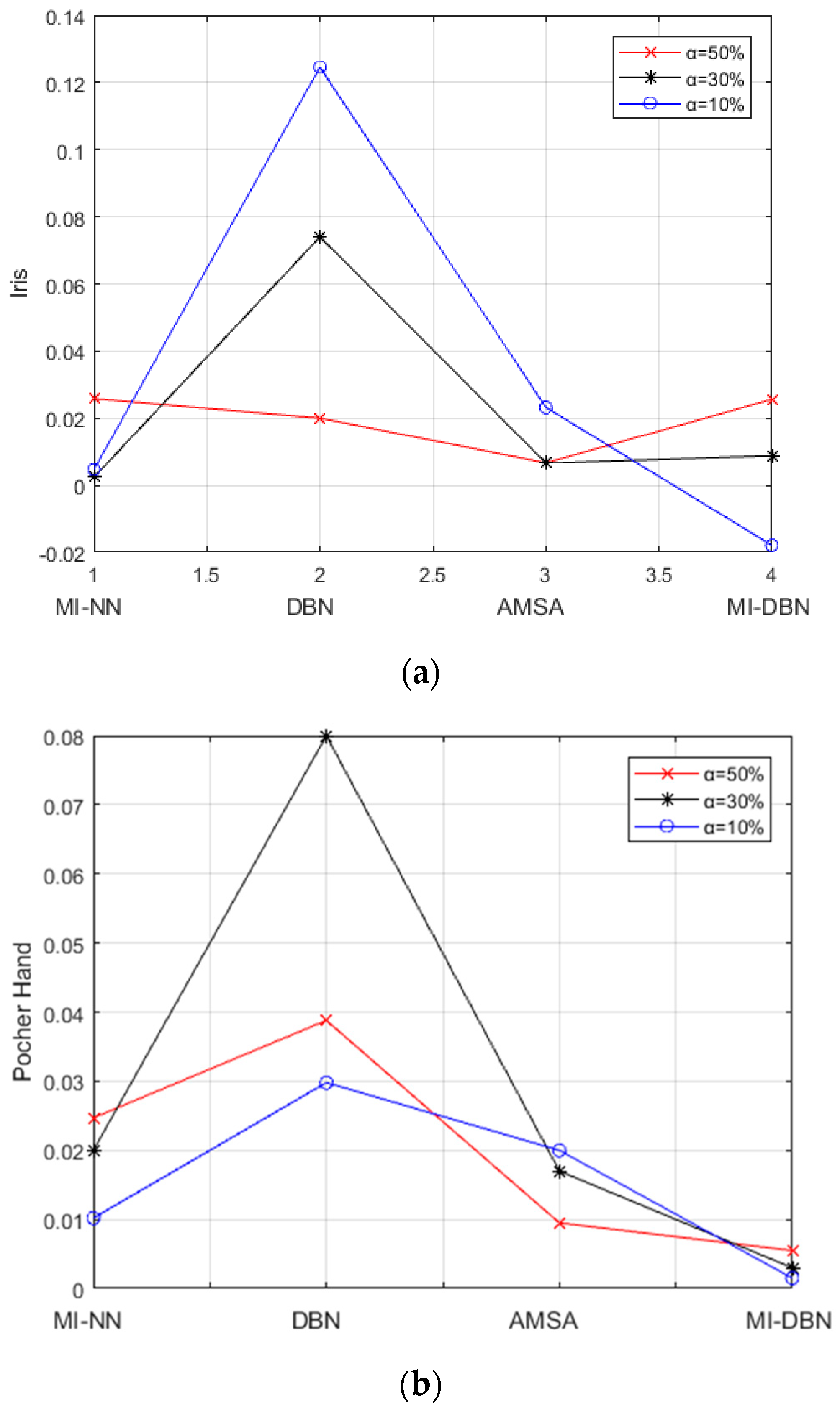To study the correlation between the performance and $\alpha$, we illustrate the difference between the two methods with varied $\alpha$ in Figure 4. According to Figure 4, there is a positive correlation between the improvement brought by the proposed method and the value of $\alpha$. The reason is that more label data leads the proposed method to absorb more useful information for classification. In contrast, this aspect does not hold true for the other algorithms.

Figure 4. Improvements over the previous methods. (a) Iris; (b) Poker Hand.

3.2. Regression

In machine learning, regression is a set of statistical processes for estimating the relationships among the variables. In this approach, the accuracy is the error rate of regression substituted by 1.

We design neural networks as regression functions to solve the regression problems in the Forest Fires dataset. For the dataset, 50% of the training samples are used for learning. In these samples, the percent of the labeled training samples $\alpha$ ranges from 10% to 50%. In the remainder of the dataset, 10% of the samples are randomly selected as test data. The constant $\lambda$ is set to –0.1.

The test accuracy on the Forest Fires dataset for NN, DBN, AMSA, MI-NN, and MI-DBN (“MI-“denotes the proposed methods) can be seen in Figure 5. The network structures used in this experiment are 13-15-1 and 13-15-17-1, which correspond to shallow networks (i.e., NN and MI-NN) and deep networks (i.e., DBN, AMSA, and MI-DBN), respectively. The activation function is sigmoid, and the output function is linear.

Figure 5. The tests of NN, MI-NN, DBN, AMSA, and MI-DBN with Forest Fires. The accuracies are plotted on the horizontal axis. (a) $\alpha =10\%$; (b) $\alpha =30\%$; (c) $\alpha =50\%$.

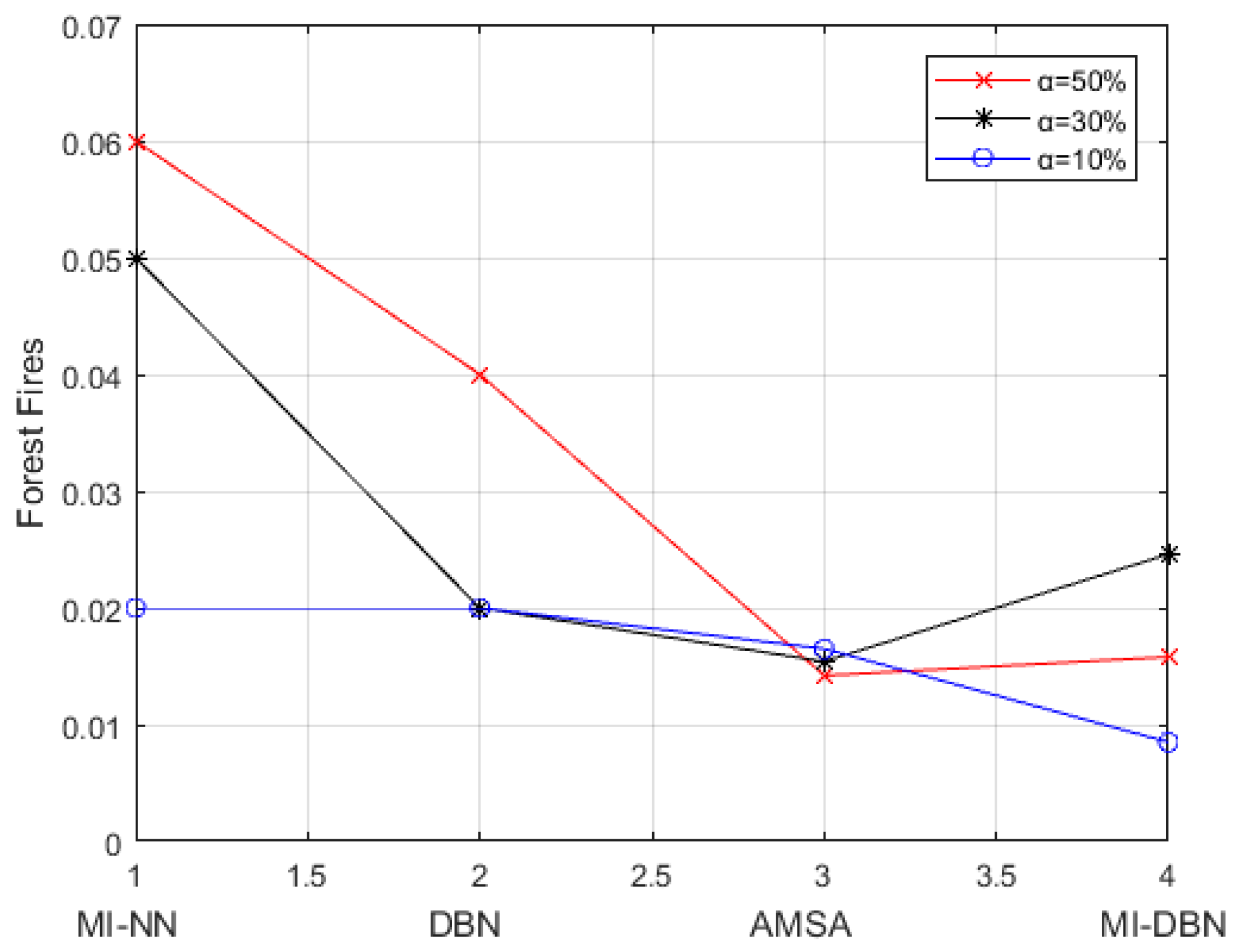
We can see that the proposed algorithm outperforms the previous methods on the dataset successfully. This finding means that the proposed algorithm can be applied to the problem of regression. In addition, the proposed algorithm improves the traditional algorithms constantly, when the percent of labeled training samples changes. To study the correlation between the performance and $\alpha$, we illustrate the difference between the two methods with varied $\alpha$ in Figure 6. According to Figure 6, there is a positive correlation between the improvement brought by the proposed method and the value of $\alpha$. The reason is that more labeled data leads the proposed method to absorb more useful information for its classification. In contrast, this aspect does not hold true for the other algorithms.

Figure 6. Improvements over previous methods.

4. Conclusions

The proposed algorithm for training neural networks is based on information theory and information geometry. The novel objective function is minimized with the theory of information geometry. The experiments show that the proposed method has better accuracy compared with the existing algorithms.