6.1. Range Next Value Query
First, we show a data structure of bits, which can be derived immediately from the existing results.
It is already known that the ORS (ORP) query on a
grid
with
k points, where all points differ in
x-coordinates, can be solved efficiently with wavelet tree [
23]. Now we describe this method in detail. The method is to build an integer array
where
is the
y-coordinate of the point whose
x-coordinate is
i. Then the ORS (ORP) query is converted to the following query on
S.
Definition 4. An integer sequence is given. Then for any interval and integer p , the range next (previous) value query returns one of the smallest (largest) elements among the ones in which are not less than p (not more than q). If there is no such element, the query should return ∅. We abbreviate it as RN (RP) query.
These queries can be efficiently solved with the wavelet tree
for
S; if
for all
, they can be solved with
rank and
select queries on
[
23]. The pseudocode for solving RN query by the wavelet tree for
S is given in Algorithm 1. In Algorithm 1,
and
stand for the left and right child of the node
v, respectively. When calling
, we can obtain the answer for the RN query with
and
p. Here a pair of the position and the value of the element is returned. If
is returned, the answer for the RN query is ∅. The RP queries on
S can be solved in a similar way using the same wavelet tree as the RN queries.
| Algorithm 1 Range Next Value by Wavelet Tree |
| 1: function RN() |
| 2: if or then return |
| 3: if then return |
| 4: |
| 5: if then |
| 6: |
| 7: if then return |
| 8: end if |
| 9: |
| 10: if then return |
| 11: else return |
| 12: end function |
The ORS query on with can be answered by solving the RN query on S with and . If the RN query returns ∅, the answer for the ORS query is also ∅. If the RN query returns an element, the answer is ∅ if the value of this element is larger than , or the point corresponding to this element otherwise. Similarly, the ORP query on can be converted to the RP query on S.
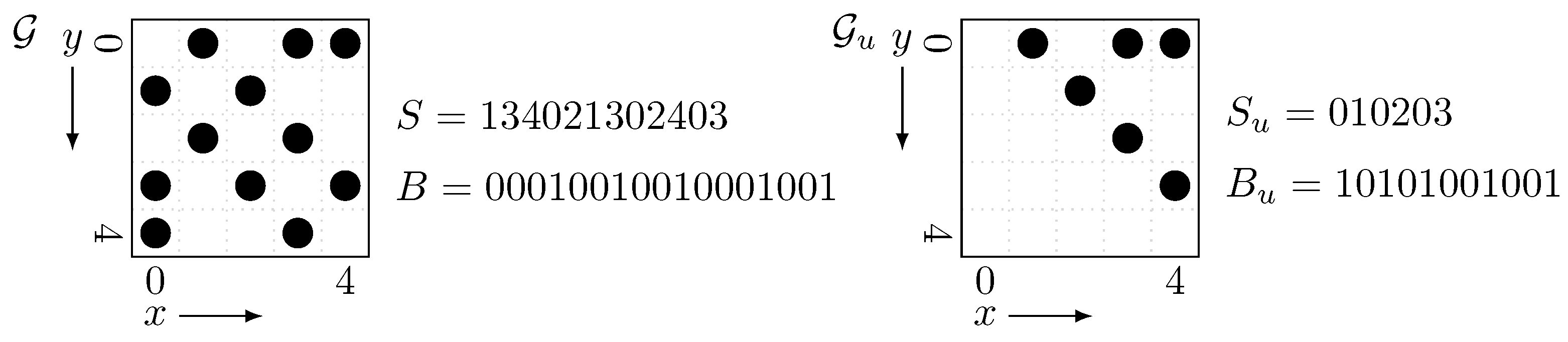
Although in the grid , on which we want to solve ORS (ORP) queries, some points share the same x-coordinate, it is addressed by preparing a bit vector B in the same way as the proof of Lemma 4. B enables us to convert x-coordinates. Here the integer sequence consists of the y-coordinates of the points on sorted by the corresponding x-coordinates. The required space of the wavelet tree is bits since there are points on and the y-coordinates vary between . Hence now we obtain a data structure of bits to solve Q and (note that the bit vector requires only bits as described in the proof of Lemma 4).
6.2. Halving Required Space
Next, we propose a data structure of
bits to solve
Q and
. The data structure shown in
Section 6.1 has information of both directions for each edge of
G since
G is an undirected graph. This seems to be redundant, thus we want to hold information of only one direction for each edge. In fact, the placement of points on
is symmetric since the adjacency matrix of
G is also symmetric. So now we consider, of the grid
, the
upper triangular part and the
lower triangular part ; a grid
inherits from
the points within the region the
x-coordinate is larger than the
y-coordinate, and
is defined in the same manner. Since
G has no self-loops,
and
have
m points for each. Now we show that we can use
as a substitute for
.
Let
be an integer sequence which contains the
y-coordinates of the points on
sorted by the corresponding
x-coordinates. Let
be a bit vector
, where
is the number of occurrences of
i in
.
enables us to convert the
x-coordinate on
to the position in
and vice versa in
time.
Figure 4 is an example of the grid
and its upper triangular part
. Here we should observe that
has half as much point as
and thus the length of
is halved from
S.
Lemma 6. Any ORS (ORP) query which appears in the reduction of Lemma 3 can be answered by solving one RN (RP) query, or by solving onerankand oneselectqueries, on .
Proof. We give a proof for only ORS queries since that for ORP queries is almost same. It can be observed that if the query rectangle of the ORS query is inside the upper triangular part of
, this ORS query can be converted to an RN query on
in the same way as
Section 6.1, since
contains all points inside the upper triangular part in
. The below claim ensures us that any ORS query related to
Q can be converted to the RN query on
.
Claim 2. The rectangles appearing in Claim 1 are all inside the upper triangular part of , i.e., these rectangles are of the form: with .
Proof. It can be easily observed that , appearing in the interval corresponding to the vertices of a subtree , equals to . Since , and thus is inside the upper triangular part. ☐
In solving , there may be query rectangles inside the lower triangular part. However, these rectangles are of the form: with . Transposing this rectangle, it is inside the upper triangular part and the problem becomes like the following: for a rectangle (with ) on , we want to know the point whose “x-coordinate” is the smallest within R. Converting the x-coordinate to the position in by , this problem is equivalent to the following problem: to find the leftmost element among ones in with a value just c.
Claim 3. Finding the leftmost element among ones in with a value just c can be done by onerankand oneselectqueries on for any .
Proof. Let . It is observed that the -st occurrence of c in is the answer if it exists and its position is in . So, if returns ∅ or a value more than then the answer is “not exist”. Otherwise the answer can be obtained by this select query itself. ☐
This completes the proof of Lemma 6. ☐
Since rank, select, RN and RP queries on can be solved in time for each with a wavelet tree for , we immediately obtain a data structure of bits for the queries Q and . Here the required space of is again bits and does not matter.
Corollary 2. There exists a data structure of bits such that for any , can be solved in time and in time. This data structure can be built in time.
Please note that the above corollary does not mention working space for the construction of the data structure. Therefore, obtaining space-efficient dynamic DFS algorithm requires consideration of the building process, since in the algorithm of Baswana et al. we need to rebuild this data structure periodically. We further consider this in
Section 7.
6.3. Range Leftmost Value Query
Next, we show another way to compress the data structure to
bits. This is achieved by solving
range leftmost (rightmost) value query with a wavelet tree. This query appears in the preliminary version [
10] of this paper. In the preliminary version, this query and the RN (RP) query (Definition 4) is used simultaneously to obtain a data structure of
bits. Although we no longer need to use this query to halve the required space as described in
Section 6.2, this query still gives us another way to compress the data structure. Moreover, this query is of independent interest since its application is beyond the dynamic DFS algorithm, as described later.
The range leftmost (rightmost) value query is defined as follows.
Definition 5. An integer sequence is given. Then for any interval and two integers , the range leftmost (rightmost) value query returns the leftmost (rightmost) element among the ones in with a value not less than p and not more than q. If there is no such element, the query should return ∅. We abbreviate it as RL (RR) query.
This RL (RR) query is a generalization of the query of Claim 3 in the sense that the value of elements we focus varies between
instead of being fixed to just
c. Moreover, the RL (RR) query is a generalization of a
prevLess query [
24], which is the RR query with
and
. It is already known that the prevLess query can be efficiently solved with the wavelet tree for
S [
24].
First we describe the idea to use RL (RR) query for solving Q and . Here we consider the symmetric variant of ORS (ORP) query, which is almost the same as ORS (ORP) query except that it returns one of the points whose “x-coordinate” is the smallest (largest) within R (we call it symmetric ORS (ORP) query). The motivation to consider symmetric ORS (ORP) queries comes from transposing the query rectangle of normal ORS (ORP) queries. Since is symmetric, the (normal) ORS query on with rectangle is equivalent to the symmetric ORS query on with rectangle . When transposing the rectangle, we can focus on the lower triangular part instead of the upper triangular part , as described below.
Let and be an integer sequence and a bit vector constructed from in the same manner as and . enables us to convert between the x-coordinate on and the position in . Then it can be observed that the symmetric ORS query on with can be answered by solving the RL query on with and , where is the interval of the position in corresponding to . If the RL query returns ∅, the answer for the symmetric ORS query is also ∅. Otherwise the answer can be obtained by converting the returned position in to the x-coordinate on by . In this reduction “leftmost” means “the smallest x-coordinate”. Similarly, a symmetric ORP query on can be converted to an RR query on . With this conversion from the symmetric ORS (ORP) query to the RL (RR) query, we can prove the following lemma which is a lower triangular version of Lemma 6.
Lemma 7. Any ORS (ORP) query which appears in the reduction of Lemma 3 can be answered by solving one RL (RR) query, or by solving onerankand oneselectqueries, on .
Proof. From Claim 2, the rectangles of the ORS queries corresponding to Q is all inside the upper triangular part. Therefore, when we transpose them, they are inside the lower triangular part. Since the symmetric ORS query can be converted into the RL query as described above, it is enough for solving Q. In solving , there may be query rectangles inside the upper triangular part. However, they are solved by one rank and one select queries on , in the same way as Claim 3. ☐
Next we describe how to solve RL (RR) queries with a wavelet tree. We prove the following lemma, by referring to the method to solve prevLess [
24] by a wavelet tree.
Lemma 8. An integer sequence is given. Suppose that for all . Then using the wavelet tree for S, both RL and RR queries can be answered in time for each.
Proof. We show that with the pseudocode given in Algorithm 2. First we show the correctness. In the arguments of , v is the node of the wavelet tree we are present, and is the interval of symbols v corresponds to (i.e., ). We claim the following, which ensures us that the answer for the RL query can be obtained by calling . ☐
Claim 4. For any node v of wavelet tree and four integers , calling yields the position of the answer for the RL query on . If the answer for the RL query is ∅, this function returns 0.
Proof. We use an induction on the depth of the node v. The base case is or (note that either of them must occur when , so if v is a leaf node the basis case must happen). For the former case, the answer is obviously ∅. For the latter case, the answer is a since all elements in have value between . In these cases, the answer is correctly returned with lines 2–3 of Algorithm 2.
Now we proceed to the general case. Let , and . Then and . Therefore, the elements in with a value between appear in the left child , and those with a value between appear in the right child . Here and can be calculated by rank queries on : and . It can be observed that the element of corresponding to the leftmost element in with a value within is also the leftmost element in with a value within . Here i can be obtained by (induction hypothesis) and . Similarly, the element of corresponding to the leftmost element in with a value within is also the leftmost element in with a value within . Again j can be obtained by (induction hypothesis) and . Hence is the leftmost element we want to know. Now the answer is correctly returned with lines 4–10 of Algorithm 2: lines 7–10 cope with the case the function returns 0. ☐
Next we discuss the time complexity when calling . We show that for each level (depth) of the wavelet tree the function visits at most four nodes. At the top level we visit only one node . At level k, the general case occurs at most two times: it may occur when contains the endpoints of . Thus, at level the function is called at most times. Since the wavelet tree has depth , function is called times. For each node, all calculation other than the recursion can be done in time, so the overall time complexity is .
The same argument can be applied for the RR query. This completes the proof. ☐
| Algorithm 2 Range Leftmost Value by Wavelet Tree |
| 1:function RL() |
| 2: if or then return 0 |
| 3: if then return a |
| 4: |
| 5: |
| 6: |
| 7: if and then return |
| 8: else if then return |
| 9: else if then return |
| 10: else return 0 |
| 11: end function |
Lemmas 7 and 8 imply another way to achieve Corollary 2.
Finally, we discuss the application of RL (RR) query beyond the dynamic DFS algorithm. Let us consider ORS and ORP queries on an
grid
whose placement of points is symmetric. Suppose that there are
d points on a diagonal line of
(we call them
diagonal points) and
points within the other part of
. Generally, there is no assumption on query rectangles such as Claim 2, so with only RN (RP) queries we cannot remove the points within the lower triangular part of
. However, using RL (RR) queries as well as RN (RP) queries, we can consider only the upper triangular and the diagonal parts of
. The idea, which is very similar to the method in the preliminary version [
10] of this paper, is as follows. First, for a query rectangle
of the ORS (ORP) query, we solve the corresponding RN (RP) query. Second, for the transposed query rectangle
, we solve the corresponding RL (RR) query, and “transpose” the answer. Finally, we combine these two answers: choose the one with smaller (larger)
y-coordinate. Let
and
be an integer sequence and a bit vector constructed from the upper triangular and the diagonal parts of
in the same manner as
and
. A wavelet tree for
can solve RN, RP, RL and RR queries on
and occupies
bits, since the diagonal part has
d points and the upper triangular part has
k points. Because the space required for
is not a matter, now we obtain a space-efficient data structure for solving ORS and ORP queries on
. If
, the required space of the data structure is actually halved from using wavelet tree directly (
bits).
If d is large, we can further compress the space from bits by treating diagonal points separately. Let be a bit vector such that if there exists a point on coordinates and otherwise. For a query rectangle , let . Then it can be easily observed that R contains diagonal lines from to if and R has no diagonal points otherwise. Therefore if , a diagonal point with smallest (largest) y-coordinate within R can be obtained by one rank and one select query on . Now we do not retain the information of the diagonal points in the wavelet tree, so the overall required space of data structures is bits.


