The Prediction of Intrinsically Disordered Proteins Based on Feature Selection

Abstract

Intrinsically disordered proteins perform a variety of important biological functions, which makes their accurate prediction useful for a wide range of applications. We develop a scheme for predicting intrinsically disordered proteins by employing 35 features including eight structural properties, seven physicochemical properties and 20 pieces of evolutionary information. In particular, the scheme includes a preprocessing procedure which greatly reduces the input features. Using two different windows, the preprocessed data containing not only the properties of the surroundings of the target residue but also the properties related to the specific target residue are fed into a multi-layer perceptron neural network as its inputs. The Adam algorithm for the back propagation together with the dropout algorithm to avoid overfitting are introduced during the training process. The training as well as testing our procedure is performed on the dataset DIS803 from a DisProt database. The simulation results show that the performance of our scheme is competitive in comparison with ESpritz and IsUnstruct.

1. Introduction

The intrinsically disordered proteins (IDPs) have at least one region lacking a unique 3D structure [1]. They exist as conformational ensembles without equilibrium positions for their atom positions and bond angles [2]. Their mobile flexibility and structural instability are encoded by their amino acid sequences [3]. They play a crucial role in a variety of important biological functions [4]. It is confirmed that some of these IDPs are related to many important regulatory functions in the cell [5], which have great impact on diseases such as Parkinson’s disease, Alzheimer’s disease and certain types of cancers [6]. Thus, accurately identifying IDPs is vital to obtaining more effective drug designs, better protein expressions and functional annotations. However, it is often difficult to purify and crystallize the disordered protein regions [7], which makes the identification of IDPs usually both expensive and time-consuming with experimental approaches [6]. Thus, it is essential to predict IDPs through the computational approaches.

For the past few decades, many computational schemes for predicting IDPs have been proposed. These schemes can be roughly classified into three categories: (1) employ the amino acid physicochemical properties and propensity scales to predict IDPs, such as FoldIndex [8], GlobPlot [9], IUPred [10], FoldUnfold [11] and IsUnstruct [12]. These schemes are based on the scale of charge/hydropathy, the relative propensity of an amino acid residue, the inter-residue contacts, and statistical physics, respectively. In particular, IsUnstruct performs well in predicting, which is an approximation of the Ising model that replaces the interaction term between neighbors with a penalty for changing between ordered and disordered states, so it is selected as a scheme of comparison in this paper. (2) Exploit machine learning techniques for the prediction of IDPs. In this category, the prediction of IDPs is considered as a binary classification problem based on many machine learning algorithms, such as artificial neural network, support vector machine and so on. The examples of this category include PONDRs [13], RONN [14], DISOPRED3 [15], BVDEA [6], DisPSSMP [16], SPINE-D [17], ESpritz [18], and so on. In this paper, we choose ESpritz as the other scheme of comparison, which is based on a bidirectional recursive neural network and also performs well in predicting. (3) Meta-approaches, such as MFDp [19], MetaPrDOS [20] and Meta-Disorder predictor [21], which use several different predictors and their trade-off to yield an optimal prediction for IDPs.

In this paper, we develop a scheme for predicting intrinsically disordered proteins which requires computing three types of features including eight structural properties, seven physicochemical properties and 20 pieces of evolutionary information. Without sacrificing our prediction accuracy of IDPs, we use a preprocessing procedure which can greatly reduce the input features and hence dramatically simplify as well as speed up identification of IDPs. Furthermore, we use two different windows to preprocess for each residue, which highlight the properties of the target residue and the surrounding around it, respectively. Thus, there are just 70 features for each residue. This number is far fewer than that of most other methods [16,17]. For training our scheme, we introduce the Adam algorithm [22] for the back propagation together with the dropout algorithm to avoid overfitting [23] in the multi-layer perceptron (MLP) neural network. The dataset DIS803 from the latest DisProt [24] database is used for training as well as testing our procedure. The dataset R80 collected by Yang et al. in [14] is used as the blind test set. Using the same input features, we compare the prediction performance of the MLP with support vector machine (SVM) [25] and Fisher discriminant [26]. The predictive results express that MLP is more appropriate to train our scheme. Finally, based on the same test sets, we compare our scheme with two competitive prediction schemes ESpritz and IsUnstruct. The simulation results show that our scheme is more accurate.

2. Materials and Methods

In this section, we propose a preprocessing procedure to preprocess three types of features with two different windows. The preprocessed features are capable of containing not only the properties of the surroundings of the target residue with the long window but also the properties related to the specific target residue with the short window. Then, for training our scheme, we employ the Adam algorithm [22] for the back propagation together with the dropout algorithm [23] to avoid overfitting.

2.1. Feature Selection

We start with a procedure of preprocessing features which contain structural and physicochemical properties as well as evolutionary information of the protein sequences. Without sacrificing our prediction accuracy of IDPs, through preprocessing, our scheme relies on only 70 features as its inputs for the identification of IDPs, which is far fewer features needed in comparison with the most of the other methods [16,17].

The selection of the structural properties including the region complexity and residue location is due to the fact that the disordered region tends to have less complexity than the ordered region [14]. To further extract the complexity information of the regions, we also add the topological entropy of a protein sequence as a novel feature for our identifying IDPs. Thus, the topological and Shannon entropy together with three amino acid propensities from GlobPlot NAR paper [9,27] are used to describe the complexity of a region around the target residue. The residue location information [28] can be obtained from computing the amino acid type, the ratio of its position in the protein sequence and the terminal position [17].

Since the IDPs and folded proteins exhibit the distinct physicochemical properties in high probability [1], we use seven physicochemical properties introduced by Jens et al. [29] for our identification. They are steric parameter, polarizability, volume, hydrophobicity, isoelectric point, helix probability and sheet probability. Finally, we also compute the Position Specific Scoring Matrix (PSSM) [16,30] through executing three iterations of PSI-BLAST (Position-Specific Iterative Basic Local Alignment Search Tool) against NCBI (National Center for Biotechnology Information) [31] non-redundant database with default parameters.

The preprocessing procedure proceeds as follows: considering a protein sequence w of length L, we choose a sliding window of odd length N ($N<L$). For the simplicity, we first transform w into a sequence of length $L+N-1$ through appending $(N-1)/2$ zeros to the both ends of w. Using the sliding window of length N, we obtain N consecutive residues ${\mathbf{w}}_j\triangleq w\left(j\right),\dots ,w(j+N-1)$ with $1\le j\le L$. For each ${\mathbf{w}}_j$ with $1\le j\le L$, we obtain

$${\mathbf{v}}_j={\left[\begin{array}{c}{m}_1\left({\mathbf{w}}_j\right)m_2\left({\mathbf{w}}_j\right)\dots m_{32}\left({\mathbf{w}}_j\right)\end{array}\right]}^{\mathrm{T}},$$

(1)

where $m_k\left({\mathbf{w}}_j\right)$ with $1\le k\le 32$ denotes the value of k-th calculated feature of ${\mathbf{w}}_j$. Without loss of generality, we assume that the block $m_k\left({\mathbf{w}}_j\right)$ with $1\le k\le 5$, $6\le k\le 12$ and $13\le k\le 32$ corresponds to the complexity features, physicochemical features and evolutionary information, respectively. Thus, each residue in the window ${\mathbf{w}}_j$ is associated with a vector ${\mathbf{v}}_j$. Sliding the window to the right one residue, we can compute ${\mathbf{v}}_{j+1}$ and associate it with every residue in the window ${\mathbf{w}}_{j+1}$. Repeat this procedure for $1\le j\le L$. Finally, every residue in the protein sequence is associated with multiple ${\mathbf{v}}_j$ with $1\le j\le L$. For each residue, we assign the average value of all the ${\mathbf{v}}_j$ with $1\le j\le L$ associated with it as the feature vector of this specific residue. Let ${\mathbf{x}}_j^{pre}(1\le j\le L)$ denote the feature vector which can be computed as

$${\mathbf{x}}_j^{pre}=\left\{\begin{array}{ccc}\frac{1}{j+(N-1)/2}{\sum }_{i=1}^{j+(N-1)/2}{\mathbf{v}}_i\hfill & ,\hfill & 1\le j\le (N-1)/2,\hfill \\ \frac{1}{N}{\sum }_{i=j-(N-1)/2}^{j+(N-1)/2}{\mathbf{v}}_i\hfill & ,\hfill & (N-1)/2<j\le L-(N-1)/2\hfill \\ \frac{1}{L-j+1+(N-1)/2}{\sum }_{i=j-(N-1)/2}^L{\mathbf{v}}_i\hfill & ,\hfill & j>L-(N-1)/2,\hfill \end{array}\right.$$

(2)

where ${\mathbf{v}}_i$ for $1\le i\le L$ is defined in Equation (1).

In Equation (1), the computation of the Shannon entropy or topological entropy can be found in [27]. For one amino acid property, $m_k\left({\mathbf{w}}_j\right)$ represents the average value of the mapped ${\mathbf{w}}_j$. In addition, the $L\times 20$ matrix $PSS{M}_w$ is used to calculate:

$$[m_{13}\left({\mathbf{w}}_j\right)\dots m_{32}\left({\mathbf{w}}_j\right)]=\frac{1}{N}\sum _{i=j}^{N+j-1}PSS{M}_w(i,1:20).$$

(3)

Finally, $35\times 1$ feature vector ${\mathbf{x}}_j(1\le j\le L)$ for each residue with one sliding window is

$${\mathbf{x}}_j=[{\mathbf{x}}_j^{loc};{\mathbf{x}}_j^{pre}],$$

(4)

with ${\mathbf{x}}_j^{loc}$ being the three pieces of location information.

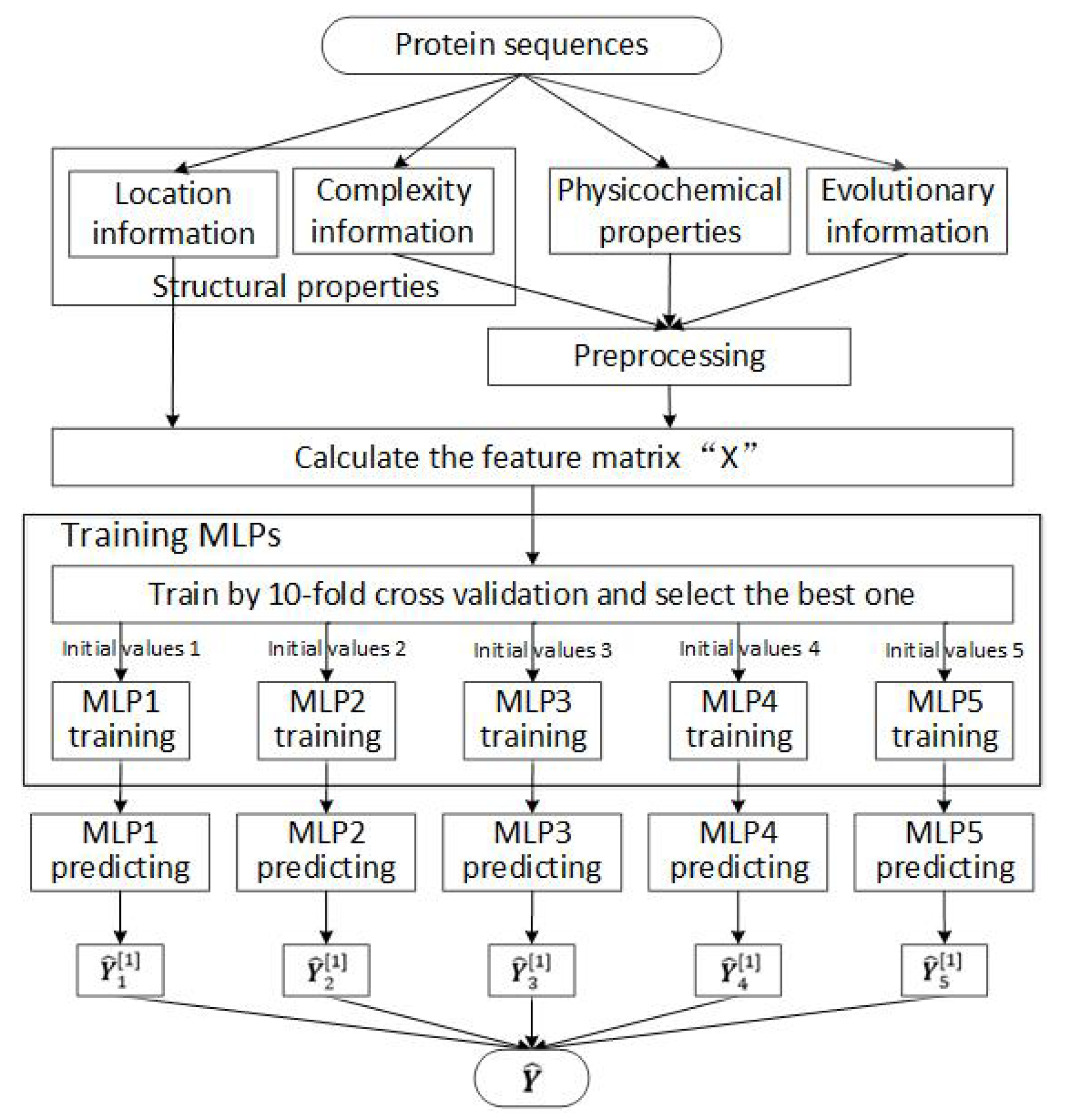
2.2. Designing and Training the MLP Neural Network

Our multi-layer perceptron (MLP) neural network structure that simultaneously takes two $35\times 1$ feature vectors ${\mathbf{x}}_j$ as its inputs is comprised of two hidden layers with each layer containing 50 perceptrons and one bias. These two $35\times 1$ input vectors with one yielded from a short window and the other from a long window. Define $\mathbf{X}=[{\mathbf{x}}_1{\mathbf{x}}_2\cdots {\mathbf{x}}_{N_s}]$ where $70\times 1$ vector ${\mathbf{x}}_j$ ($1\le j\le N_s$) is computed from Equation (4) with $N_s$ being the total number of all the samples. Let $\mathbf{Y}$ be the $2\times N_s$ output matrix whose column is equal to either ${[1,0]}^T$ or ${[0,1]}^T$ corresponding to the disordered or ordered residue. The training process proceeds as follows:

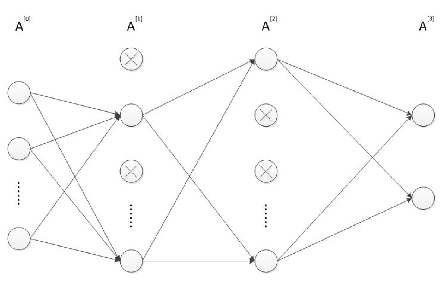
• Input $\mathbf{X}$ and compute the forward propagation through

  $$\begin{array}{ccc}\hfill {\mathbf{Z}}^{\left[l\right]}& =& {\mathbf{W}}^{\left[l\right]}·{\mathbf{A}}^{[l-1]}+{\mathbf{b}}^{\left[l\right]},\hfill \end{array}$$

  (5)

  $$\begin{array}{ccc}\hfill {\mathbf{A}}^{\left[l\right]}& =& {\mathrm{g}}^{\left[l\right]}({\mathbf{Z}}^{\left[l\right]})\ast \mathbf{R}\left(p_d\right),\hfill \end{array}$$

  (6)

  where ${\mathrm{g}}^{\left[l\right]}$ is the activation function in the l-th layer $(l=1,2,3)$. In our MLP neural network, both ${\mathrm{g}}^{\left[1\right]}$ and ${\mathrm{g}}^{\left[2\right]}$ are ReLU functions and ${\mathrm{g}}^{\left[3\right]}$ is softmax function. $\mathbf{R}\left(p_d\right)$ represents the dropout vector which obeys the Bernoulli distribution with probability $p_d$. The symbols ∗ and · respectively represent the scalar and matrix multiplication. Furthermore, ${\mathbf{A}}^{\left[0\right]}$ is equal to $\mathbf{X}$ while ${\mathbf{A}}^{\left[3\right]}$ is the prediction result $\widehat{\mathbf{Y}}$. The structure of the MLP network is shown in Figure 1.
  

  Figure 1. The structure of the MLP network.
• After obtaining $\widehat{\mathbf{Y}}$, compute the cost function which is the cross entropy. If the cost function is converged or the max iteration number is achieved, then stop and output $\widehat{\mathbf{Y}}$.
• Employ Adam algorithm [22] to perform the back propagation. Update $\mathbf{W}$ and $\mathbf{b}$ and repeat 1.

The detail paradigm of our scheme is shown in Figure 2. Based on the feature matrix $\mathbf{X}$, we use 10-fold cross validation to train MLP networks, and select the best one according to their prediction results. Then, to reduce the impact of initial values, five different random initial values are used to train five independent MLP networks. Finally, the prediction results are obtained by averaging the outputs of these five trained MLP networks.

Figure 2. The detail paradigm of our scheme.

2.3. Datasets for Training and Testing

The dataset DIS803 from the latest version of DisProt [24] is used in our training and testing. The DIS803 is comprised of 803 protein sequences with 1254 disordered regions and 1343 ordered regions, which corresponds to 92,418 disordered and 315,856 ordered residues, respectively. We randomly split this dataset into two subsets of data with the ratio of 9:1. The larger one containing 721 protein sequences uses as the training set by 10-fold cross validation. The training set contains 85,184 disordered and 289,983 ordered residues. The test set has 82 protein sequences, which corresponds to 7234 disordered and 25,873 ordered residues. In addition, we also use the dataset R80 as the blind test set. Dataset R80 is collected by Yang et al. in [14], which is comprised of 80 protein sequences with 183 disordered regions and 151 ordered regions.

2.4. Performance Evaluation

The performance of our scheme is evaluated by four metrics [32] which contain sensitivity ($Sens$), specificity ($Spec$), the weighted score ($Sw$) and Matthews correlation coefficient ($MCC$). We use $TP$, $TN$, $FN$ and $FP$ to correspond to the number of true positives, true negatives, false negatives and false positives, where positive is disorder and negative is order. The $MCC$ and $Sw$ can be computed as follows:

$$MCC=\frac{(TP\times TN)-(FP\times FN)}{\sqrt{(TP+FP)(TP+FN)(TN+FP)(TN+FN)}},$$

(7)

$$Sw=Sens+Spec-1,$$

(8)

where $Sens=TP/(TP+FN)$ and $Spec=TN/(TN+FP)$.

3. Results and Discussion

The simulation results show that our scheme yields better weighted scores in comparison with ESpritz and IsUnstruct based on the test set from DisProt [24] and the blind test set R80.

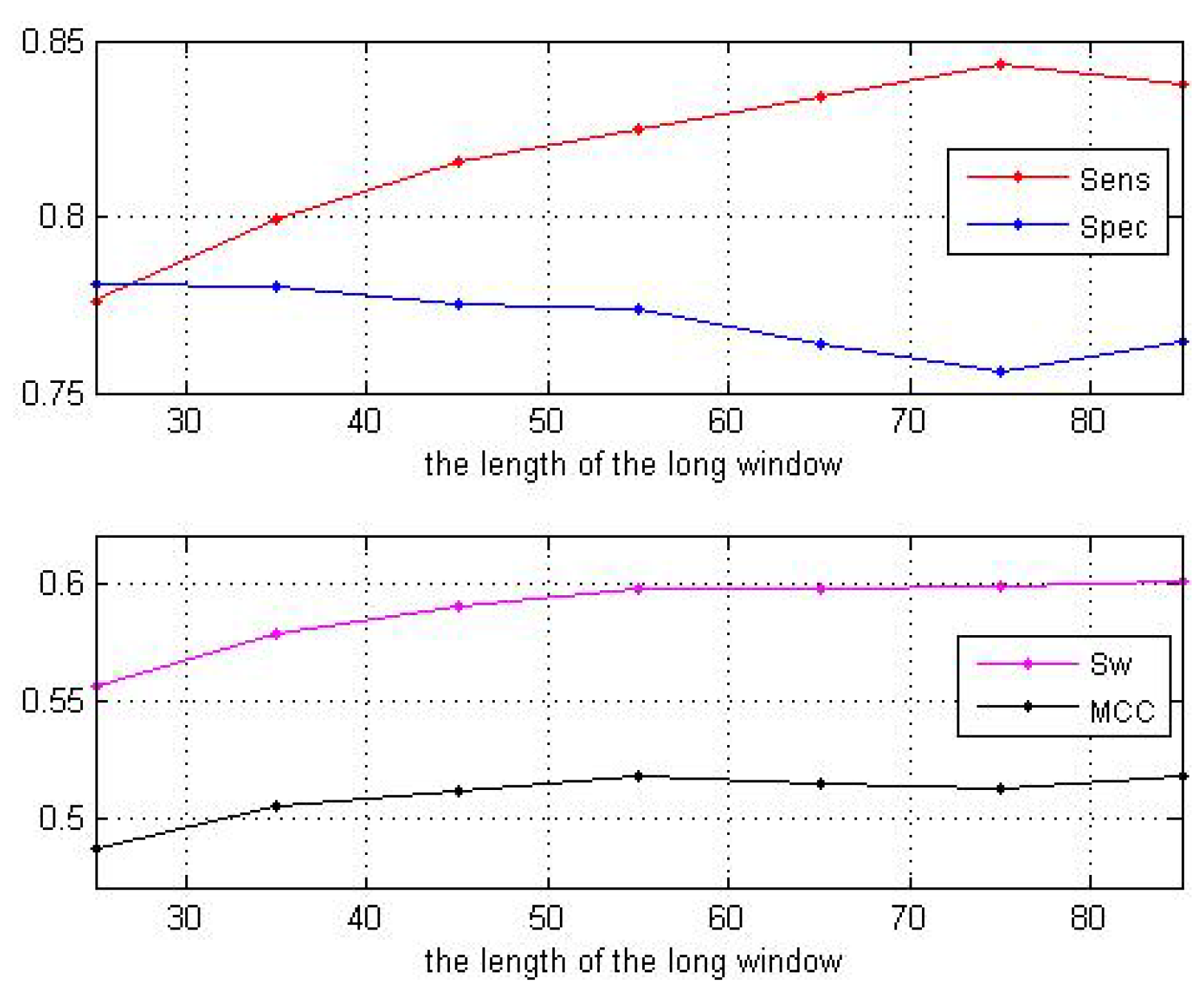
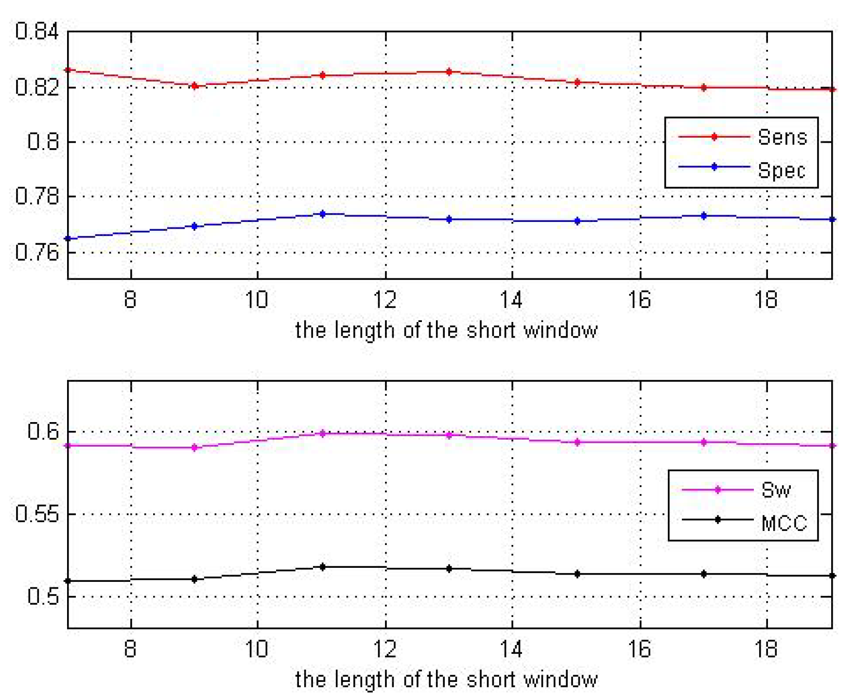
3.1. Impact of the Sliding Window Sizes

Since the input of our scheme is comprised of the information obtained from a short window as well as a long window, we choose different window sizes to study the impact of window sizes on the training set of our scheme. The MLP neural network contains two hidden layers with each layer containing 50 perceptrons and one bias. We set the dropout parameter $p_d$ to be $0.5$ with the learning rate being $0.0001$.

Fixing the size of the short window at 11, Table 1 shows the predictive performance of various long windows based on the training set with 10-fold cross validation.

Table 1. Performance with different long windows.

Window Sizes	25	35	45	55	65	75	85
$Sens$	0.7762	0.7991	0.8156	0.8245	0.8344	0.8430	0.8373
$Spec$	0.7806	0.7805	0.7752	0.7739	0.7637	0.7556	0.7645
$Sw$	0.5568	0.5796	0.5908	0.5984	0.5980	0.5990	0.6018
$MCC$	0.4872	0.5053	0.5124	0.5181	0.5147	0.5133	0.5180

When the size of the long window is larger than 55, the curves of the two parameters $Sw$ and $MCC$ tend to be stable as shown in Figure 3. Thus, we set the size to be 55. Next, fixing the size of the long window at 55, we change the size of the short window. The predictive performance is shown in Table 2 as well as Figure 4. These results show that our choice of window size 11 is acceptable.

Figure 3. Performance with different long windows.

Table 2. Performance with different short windows.

Window Sizes	7	9	11	13	15	17	19
$Sens$	0.8264	0.8204	0.8245	0.8254	0.8221	0.8199	0.8191
$Spec$	0.7649	0.7694	0.7738	0.7718	0.7714	0.7734	0.7722
$Sw$	0.5913	0.5898	0.5984	0.5972	0.5933	0.5933	0.5913
$MCC$	0.5096	0.5098	0.5181	0.5165	0.5131	0.5139	0.5119

Figure 4. Performance with different short windows.

3.2. Impact of the MLP Parameters

We set the sizes of the short and long window respectively to be 11 and 55. We change the parameters of the MLP neural network to investigate the influence of these parameters on the training set with 10-fold cross validation.

Firstly, we change the number of perceptrons in hidden layers. We use $N_{neur}$ to denote the number of perceptrons in each hidden layer. Table 3 shows the predictive results of $N_{neur}=[50,25],[50,50],[100,50]$ with the same dropout parameter $p_d=0.5$ and learning rate $0.0001$. From Table 3, considering that $N_{neur}=[50,50]$ and $N_{neur}=[100,50]$ obtain almost the same $Sw$ and $MCC$, as well as $N_{neur}=[50,50]$ using fewer perceptrons, we still select $N_{neur}=[50,50]$. Next, with $N_{neur}=[50,50],$ we vary the value of $p_d$ to analyze the influence of different dropout parameters on the predictive performance. Table 4 shows the results of $p_d=0.5,0.7,1$. In Table 4, as the value of $p_d$ increases, which means that the degree of dropout decreases, the $Sw$ shows a downward trend. Taking the values of these four evaluation parameters into consideration, we select $p_d=0.5$.

Table 3. Performance with different $N_{neur}$.

Nneur1	$\mathit{Sens}$	$\mathit{Spec}$	$\mathit{Sw}$	$\mathit{MCC}$
$[50,25]$	0.8291	0.7679	0.5967	0.5148
$[50,50]$	0.8245	0.7739	0.5984	0.5181
$[100,50]$	0.8237	0.7749	0.5986	0.5186

Table 4. Performance with different $p_d$.

${\mathit{p}}_{\mathit{d}}$	$\mathit{Sens}$	$\mathit{Spec}$	$\mathit{Sw}$	$\mathit{MCC}$
$0.5$	0.8245	0.7739	0.5984	0.5181
$0.7$	0.8231	0.7676	0.5907	0.5100
1	0.7633	0.8106	0.5738	0.5123

3.3. Impact of the Preprocessing

After determining the parameters of MLP, we analyze the impact of the preprocessing procedure. If we directly take the features in the sliding window as the input of the target residue without preprocessing, the input features will contain a lot of redundant information. It is expected to improve the predictive performance by reducing the dimension of features and improving the effectiveness of features, which is exactly the role of preprocessing.

Without preprocessing, the feature dimensions are 335 and 1655 in the windows of 11 and 55, respectively. Thus, the feature dimension of input is 1990 for each residue. However, after preprocessing, the feature dimension of input is greatly reduced to 70, but the input feature still contains the main information of both the target residue and the its surroundings. Table 5 shows the performance comparison of the schemes with and without preprocessing based on the training set with 10-fold cross validation. These results indicate that the performance of the scheme with preprocessing outperforms the scheme without preprocessing.

Table 5. Performance comparison of the schemes with and without preprocessing.

Schemes	$\mathit{Sens}$	$\mathit{Spec}$	$\mathit{Sw}$	$\mathit{MCC}$
With preprocessing	0.8245	0.7739	0.5984	0.5181
Without preprocessing	0.7291	0.7723	0.5014	0.4399

3.4. Impact of the Evolutionary Information

In this paper, we extract evolutionary information from the Position Specific Scoring Matrix (PSSM) which can improve the predictive accuracy but increase the execution time at the same time. However, both the accuracy and speed of the prediction are important. Table 6 displays the performance comparison of our scheme excluding or including PSSM based on the training set with 10-fold cross validation.

Table 6. Performance comparison of the schemes excluding and including PSSM.

Schemes	$\mathit{Sens}$	$\mathit{Spec}$	$\mathit{Sw}$	$\mathit{MCC}$	Speed(s)
Including PSSM	0.8245	0.7739	0.5984	0.5181	1340.0
Excluding PSSM	0.7508	0.7809	0.5317	0.4671	2.9160

Moreover, in order to compare the execution time, we select a sequence (DP01011) to calculate the execution time of each situation as shown in Table 6. Although using PSSM will increase the execution time, it significantly improves the accuracy of prediction in our scheme. Thus, we still include PSSM information in the input features.

3.5. Comparing with Other Classification Algorithms

Based on the same input, we compare the trained multi-layer perceptron (MLP) with other two classification algorithms support vector machine (SVM) and Fisher discriminant. The principle of SVM is to find a hyperplane that maximizes the interval between two categories of samples [25]. It can be transformed to solve a quadratic programming problem. We use a SVM with radial basis function (RBF) Gaussian kernel to contrast. Fisher discriminant is a linear classification algorithm. It maximizes the generalized Rayleigh entropy to search the optimal projection direction [26]. Table 7 shows the predictive results of MLP, SVM and Fisher discriminant, based on the training set with 10-fold cross validation.

Table 7. Performance comparison with SVM and Fisher discriminant.

Schemes	$\mathit{Sens}$	$\mathit{Spec}$	$\mathit{Sw}$	$\mathit{MCC}$
MLP	0.8245	0.7739	0.5984	0.5181
SVM	0.7643	0.7765	0.5408	0.4729
Fisher	0.8127	0.7660	0.5787	0.5000

It is obvious that MLP obtains better $Sw$ and $MCC$ in Table 7. Therefore, based on the same preprocessed features as input, MLP is more appropriate to train our scheme.

3.6. Testing Performances

In this section, using the same test sets, we compare our scheme, named DISpre, with two competitive schemes ESpritz and IsUnstruct. Table 8 shows the predictive performance of these three schemes on the test set from the latest version of DisProt [24]. The results of the ESpritz and IsUnstruct are obtained from their online predictors.

Table 8. Performance comparison with existing schemes on the test set from DisProt.

Schemes	$\mathit{Sens}$	$\mathit{Spec}$	$\mathit{Sw}$	$\mathit{MCC}$
DISpre	0.7910	0.7836	0.5746	0.5006
ESpritz	0.7255	0.8135	0.5389	0.4840
IsUnstruct	0.7513	0.7855	0.5368	0.4711

From Table 8, our scheme DISpre gets the best $Sens$ and ESpritz gets the best $Spec$. However, DISpre also yields better $Sw$ and $MCC$ than ESpritz and IsUnstruct on the test set. In addition, we also compare these three schemes on the blind test set R80 as shown in Table 9. In this dataset, our scheme still obtains better $Sens$ and $Sw$.

Table 9. Performance comparison with existing schemes on R80 set.

Schemes	$\mathit{Sens}$	$\mathit{Spec}$	$\mathit{Sw}$	$\mathit{MCC}$
DISpre	0.7482	0.8618	0.6100	0.4707
ESpritz	0.6884	0.9115	0.6000	0.5178
IsUnstruct	0.6882	0.8845	0.5727	0.4663

4. Conclusions

In this paper, we present a new scheme for predicting intrinsically disordered proteins. Our scheme uses three types of features including eight structural properties, seven physicochemical properties and 20 pieces of evolutionary information. Furthermore, we employ a preprocessing procedure which greatly reduces the input features. With two different windows, the preprocessed features are capable of containing not only the properties of the surroundings of the target residue with the long window but also the properties related to the specific target residue with the short window. We also use the Adam algorithm for the back propagation together with the dropout algorithm to avoid overfitting in training our scheme. Comparing with SVM and Fisher discriminant, the predictive results express that MLP is more appropriate to train our scheme. Finally, based on the same test sets, the simulation results show that our scheme obtains better $Sw$ than two competitive schemes ESpritz and IsUnstruct.

References

- Uversky, V.N. The mysterious unfoldome: structureless, underappreciated, yet vital part of any given proteome. J. Biomed. Biotechnol. 2010, 2010, 568068. [Google Scholar] [CrossRef] [PubMed]
- Dunker, A.K.; Kriwacki, R.W. The orderly chaos of proteins. Sci. Am. 2011, 304, 68–73. [Google Scholar] [CrossRef] [PubMed]
- Oldfield, C.J.; Dunker, A.K. Intrinsically Disordered Proteins and Intrinsically Disordered Protein Regions. Annu. Rev. Biochem. 2014, 83, 553–584. [Google Scholar] [CrossRef] [PubMed]
- Uversky, V.N. Functional roles of transiently and intrinsically disordered regions within proteins. FEBS J. 2015, 282, 1182–1189. [Google Scholar] [CrossRef] [PubMed]
- Wright, P.E.; Dyson, H.J. Intrinsically unstructured proteins: Re-assessing the protein structure-function paradigm. J. Mol. Biol. 1999, 293, 321–331. [Google Scholar] [CrossRef]
- Kaya, I.E.; Ibrikci, T.; Ersoy, O.K. Prediction of disorder with new computational tool: BVDEA. Expert Syst. Appl. 2011, 38, 14451–14459. [Google Scholar] [CrossRef]
- Oldfield, C.J.; Ulrich, E.L.; Cheng, Y.G.; Dunker, A.K.; Markley, J.L. Addressing the intrinsic disorder bottleneck in structural proteomics. Proteins 2005, 59, 444–453. [Google Scholar] [CrossRef] [PubMed]
- Prilusky, J.; Felder, C.E.; Zeev-Ben-Mordehai, T.; Rydberg, E.H.; Man, O.; Beckmann, J.S.; Silman, I.; Sussman, J.L. FoldIndex: A simple tool to predict whether a given protein sequence is intrinsically unfolded. Bioinformatics 2005, 21, 3435–3438. [Google Scholar] [CrossRef]
- Linding, R.; Russell, R.B.; Neduva, V.; Gibson, T.J. Globplot: Exploring Protein Sequences for Globularity and Disorder. Nucleic Acids Res. 2003, 31, 3701–3708. [Google Scholar] [CrossRef]
- Dosztanyi, Z.; Csizmok, V.; Tompa, P.; Simon, I. IUPred: Web server for the prediction of intrinsically unstructured regions of proteins based on estimated energy content. Bioinformatics 2005, 21, 3433–3434. [Google Scholar] [CrossRef]
- Galzitskaya, O.V.; Garbuzynskiy, S.O.; Lobanov, M.Y. FoldUnfold: web server for the prediction of disordered regions in protein chain. Bioinformatics 2006, 22, 2948–2949. [Google Scholar] [CrossRef]
- Lobanov, M.Y.; Galzitskaya, O.V. The Ising model for prediction of disordered residues from protein sequence alone. Phys. Biol. 2011, 8, 1–9. [Google Scholar] [CrossRef] [PubMed]
- PONDR: Predictors of Natural Disordered Regions. Available online: http://www.pondr.com/ (accessed on 20 February 2019).
- Yang, Z.R.; Thomson, R.; McNeil, P.; Esnouf, R.M. RONN: The bio-basis function neural network technique applied to the detection of natively disordered regions in proteins. Bioinformatics 2005, 21, 3369–3376. [Google Scholar] [CrossRef]
- Ward, J.J.; Sodhi, J.S.; Mcguffin, L.J.; Buxton, B.F.; Jones, D.T. Prediction and Functional Analysis of Native Disorder in Proteins from the Three Kingdoms of Life. J. Mol. Biol. 2004, 337, 635–645. [Google Scholar] [CrossRef] [PubMed]
- Su, C.T.; Chen, C.Y.; Ou, Y.Y. Protein disorder prediction by condensed pssm considering propensity for order or disorder. BMC Bioinform. 2006, 7, 319. [Google Scholar] [CrossRef]
- Zhang, T.; Faraggi, E.; Xue, B.; Dunker, A.K.; Uversky, V.N.; Zhou, Y. SPINE-D: Accurate prediction of short and long disordered regions by a single neural-network based method. J. Biomol. Struct. Dyn. 2012, 29, 799–813. [Google Scholar] [CrossRef]
- Walsh, I.; Martin, A.J.; Di Domenico, T.; Tosatto, S.C. ESpritz: Accurate and fast prediction of protein disorder. Bioinformatics 2012, 28, 503–509. [Google Scholar] [CrossRef] [PubMed]
- Mizianty, M.J.; Stach, W.; Chen, K.; Kedarisetti, K.D.; Disfani, F.M.; Kurgan, L. Improved sequence-based prediction of disordered regions with multilayer fusion of multiple information sources. Bioinformatics 2010, 26, i489–i496. [Google Scholar] [CrossRef]
- Ishida, T.; Kinoshita, K. Prediction of disordered regions in proteins based on the meta approach. Bioinformatics 2008, 24, 1344–1348. [Google Scholar] [CrossRef]
- Schlessinger, A.; Punta, M.; Yachdav, G.; Kajan, L.; Rost, B. Improved disorder prediction by combination of orthogonal approaches. PLoS ONE 2009, 4, 4433. [Google Scholar] [CrossRef]
- Kingma, D.P.; Ba, J.L. Adam: A method for stochastic optimization. In Proceedings of the 3rd International Conference on Learning Representations (ICLR), San Diego, CA, USA, 7 May 2015; pp. 1–15. [Google Scholar]
- Srivastava, N.; Hinton, G.; Krizhevsky, A.; Sutskever, I.; Salakhutdinov, R. Dropout: A Simple Way to Prevent Neural Networks from Overfitting. J. Mach. Learn. Res. 2014, 15, 1929–1958. [Google Scholar]
- Sickmeier, M.; Hamilton, J.A.; LeGall, T.; Vacic, V.; Cortese, M.S.; Tantos, A.; Szabo, B.; Tompa, P.; Chen, J.; Uversky, V.N.; et al. DisProt: the database of disordered proteins. Nucleic Acids Res. 2007, 35, 786–793. [Google Scholar] [CrossRef] [PubMed]
- Burges, C.J.C. A tutorial on support vector machines for pattern recognition. Data Min. Knowl. Discov. 1998, 2, 121–167. [Google Scholar] [CrossRef]
- Mika, S.; Ratsch, G.; Weston, J.; Scholkopf, B.; Mullers, K.R. Fisher discriminant analysis with kernels. In Proceedings of the Neural Networks for Signal Processing IX: Proceedings of the 1999 IEEE Signal Processing Society Workshop, Madison, WI, USA, 25 August 1999; pp. 41–48. [Google Scholar]
- He, H.; Zhao, J.X. A Low Computational Complexity Scheme for the Prediction of Intrinsically Disordered Protein Regions. Math. Probl. Eng. 2018, 2018, 8087391. [Google Scholar] [CrossRef]
- Shimizu, K.; Muraoka, Y.; Hirose, S.; Noguchi, T. Feature selection based on physicochemical properties of redefined n-term region and c-term regions for predicting disorder. In Proceedings of the 2005 IEEE Symposium on Computational Intelligence in Bioinformatics and Computational Biology, La Jolla, CA, USA, 15 November 2005; pp. 262–267. [Google Scholar]
- Meiler, J.; Muller, M.; Zeidler, A.; Schmaschke, F. Generation and evaluation of dimension-reduced amino acid parameter representations by artificial neural networks. J. Mol. Model. 2001, 7, 360–369. [Google Scholar] [CrossRef]
- Jones, D.T.; Ward, J.J. Prediction of Disordered Regions in Proteins from Position Specific Score Matrices. Proteins 2003, 3, 573–578. [Google Scholar] [CrossRef] [PubMed]
- Pruitt, K.D.; Tatusova, T.; Klimke, W.; Maglott, D.R. NCBI Reference Sequences: current status, policy and new initiatives. Nucleic Acids Res. 2009, 37, 32–35. [Google Scholar] [CrossRef] [PubMed]
- Monastyrskyy, B.; Fidelis, K.; Moult, J.; Tramontano, A.; Kryshtafovych, A. Evaluation of disorder predictions in CASP9. Proteins 2011, 79, 107–118. [Google Scholar] [CrossRef]
© 2019 by the authors. Licensee MDPI, Basel, Switzerland. This article is an open access article distributed under the terms and conditions of the Creative Commons Attribution (CC BY) license (http://creativecommons.org/licenses/by/4.0/).