Integrated Speed Planning and Friction Coefficient Estimation Algorithm for Intelligent Electric Vehicles

Abstract

To improve the safety of intelligent electric vehicles and avoid side slipping on curved roads with changing friction coefficients, an integrated speed planning and friction coefficient estimation algorithm is proposed. With this algorithm, the speeds of intelligent electric vehicles can be planned online using estimated road friction coefficients to avoid lane departures. When a decrease in the friction coefficient is detected on a curved road with a large curvature, the algorithm will plan a low and safe speed to avoid side slipping. When a normal friction coefficient is detected, the algorithm will plan a higher speed for normal driving. Simulations using MATLAB and CarSim have been performed to demonstrate the effectiveness of the designed algorithm. The simulation results suggest that the proposed algorithm is applicable to speed planning on curved roads with changing friction coefficients.

1. Introduction

With the rapid development of vehicle technology [1,2,3], considerable attention has been devoted to intelligent vehicles [4,5,6]. Various technologies have been investigated to satisfy the demanding requirements of commercialization. In particular, lane keeping systems (LKSs) and cruise control are two fundamental technologies for intelligent vehicles. A number of studies have been performed in these critical areas [7,8,9,10,11,12,13,14,15,16,17,18,19,20,21,22]. A nested proportional-integral-derivative (PID) algorithm with two closed loops was presented for lane keeping in [7]. A super-twisting sliding mode scheme was suggested in [8] to eliminate vehicle lateral tracking error and handle the chatting phenomenon. Three kinds of sliding mode control algorithms were suggested and compared with regard to the actuator saturation scenario in [9]. In [10], a control algorithm consisting of inner and outer loops in the control system was proposed for an LKS based on sliding mode control. In [11], the authors addressed the problem of integrated direct yaw moment control and front steering for an LKS with a transfer function. In [23], a proportional-type space-learning control scheme was constructed for vehicle path tracking, and a stability analysis of the proposed scheme was also performed. In [12], to achieve guaranteed lane keeping and speed tracking performance, a motion controller was developed based on fuzzy model predictive control. In [13], to consider nonlinear vehicle dynamics, a cruise control algorithm was proposed using nonlinear model predictive control. In [14], a self-learning cruise control scheme, in which the system parameters can be adjusted online, was developed for speed tracking. In [15], using a fractional linear feedforward prefilter, a cruise control method was designed considering an acceleration signal. In [16], a cruise controller was constructed considering energy consumption. In [17], the development of cruise control at a motor company was described. In [18], a crone feedback control strategy was extended to a cruise control application. In [19], a super-twisting sliding mode algorithm with adaptive gains was used in the design of a cruise controller. In [20], a cruise controller was proposed based on a fuzzy PID control method. In [21], a piecewise method was used in the development of a cruise control system. In [22], an online learning fuzzy scheme was considered when developing a cruise control system. In [24], an indirect field-oriented control algorithm was proposed for electric vehicles considering the motor uncertainty. Simulations and experiments have shown that the algorithms proposed in these studies are effective for lane keeping or cruise control on normal roads; thus, these investigations have been useful in the development of intelligent vehicles.

Most of these studies have focused on normal roads with constant friction coefficients. However, due to changes in weather or the traffic environment, the friction coefficient may be reduced in real situations. For instance, water or ice on the road surface may significantly decrease the friction coefficient, causing the handling performance of a vehicle on a curved road to degrade. At high speeds, the lane keeping performance may not be maintained due to the limited adhesion on a curved road with a low friction coefficient; however, this concern has seldom been considered in previous studies on lane keeping and cruise control technologies. Thus, it is essential to develop an algorithm that can be used for online speed planning based on estimated friction coefficients. On a curved road with a high curvature and a low friction coefficient, such an algorithm can plan a lower speed to ensure safety.

The aim of this paper is to design an integrated speed planning and friction coefficient estimation algorithm to address changing friction coefficients on curved roads to avoid potential accidents. Two key points should be considered in regard to such road conditions. First, the friction coefficients should be estimated online to provide information about the road surface. Second, the vehicle speed should be planned based on these estimated friction coefficients. On a normal road with a high friction coefficient, a constant desired speed is preferred. When a decrease in the friction coefficient is detected, a safe speed should be planned to avoid side slipping and accidents on curved roads with large curvatures. In this paper, a friction coefficient estimation algorithm is proposed based on torque injection [25,26]. By means of torque injection, the slip ratios of the tires can be increased, which is essential for accurately estimating the friction coefficient. The friction coefficient is estimated based on the slip ratios and side-slip angles over a given sampling period. With the aim of calculating a safe vehicle speed, a speed planning algorithm is proposed that considers a changing friction coefficient on a curved road. The speed profile is planned to prevent potential accidents caused by high speeds and the saturation of friction on curved roads with changing friction coefficients, which is a topic that has seldom been discussed in previous studies.

By combining the proposed speed-planning and friction coefficient estimation algorithms, an integrated speed-planning and friction coefficient estimation (ISPFCE) algorithm is proposed. This algorithm consists of two components, as shown in Figure 1. Note that the sensor system, motion controller, and electric vehicle are also included in this figure to illustrate the overall relationships in the system. The first component of the algorithm is the friction coefficient estimation, in which the friction coefficient is estimated through optimization. The second component is the speed planning, which is designed to calculate a safe speed considering the desired speed and safety constraints. A motion controller is used for lane keeping and cruise control; however, this controller is not the focus of this study. Thus, the designed algorithm can be utilized in combination with various motion controllers based on previously-designed lane-keeping and cruise control algorithms to improve their performance.

The remainder of this paper is organized as follows. In Section 2, the friction estimation algorithm based on torque injection is proposed. In Section 3, the speed-planning method considering the road curvature and friction coefficient is presented. Simulations conducted to verify the proposed algorithm are reported in Section 4. Finally, conclusions are presented in Section 5.

2. Friction Coefficient Estimation

The friction coefficient estimation algorithm, which serves as the basis for speed planning, is proposed in this section. As shown in Figure 2, the proposed algorithm has four components. The first component is the tire force and effective radius estimation, in which the longitudinal, lateral, and vertical forces, as well as the effective radius of each tire are estimated. The second component is the calculation of the tire side-slip angles and slip ratios, which are calculated for each tire. The third component is the calculation of the friction coefficient, which produces the final estimated friction coefficient. The last component is torque injection [25,26], which involves calculating the drive torque to be injected.

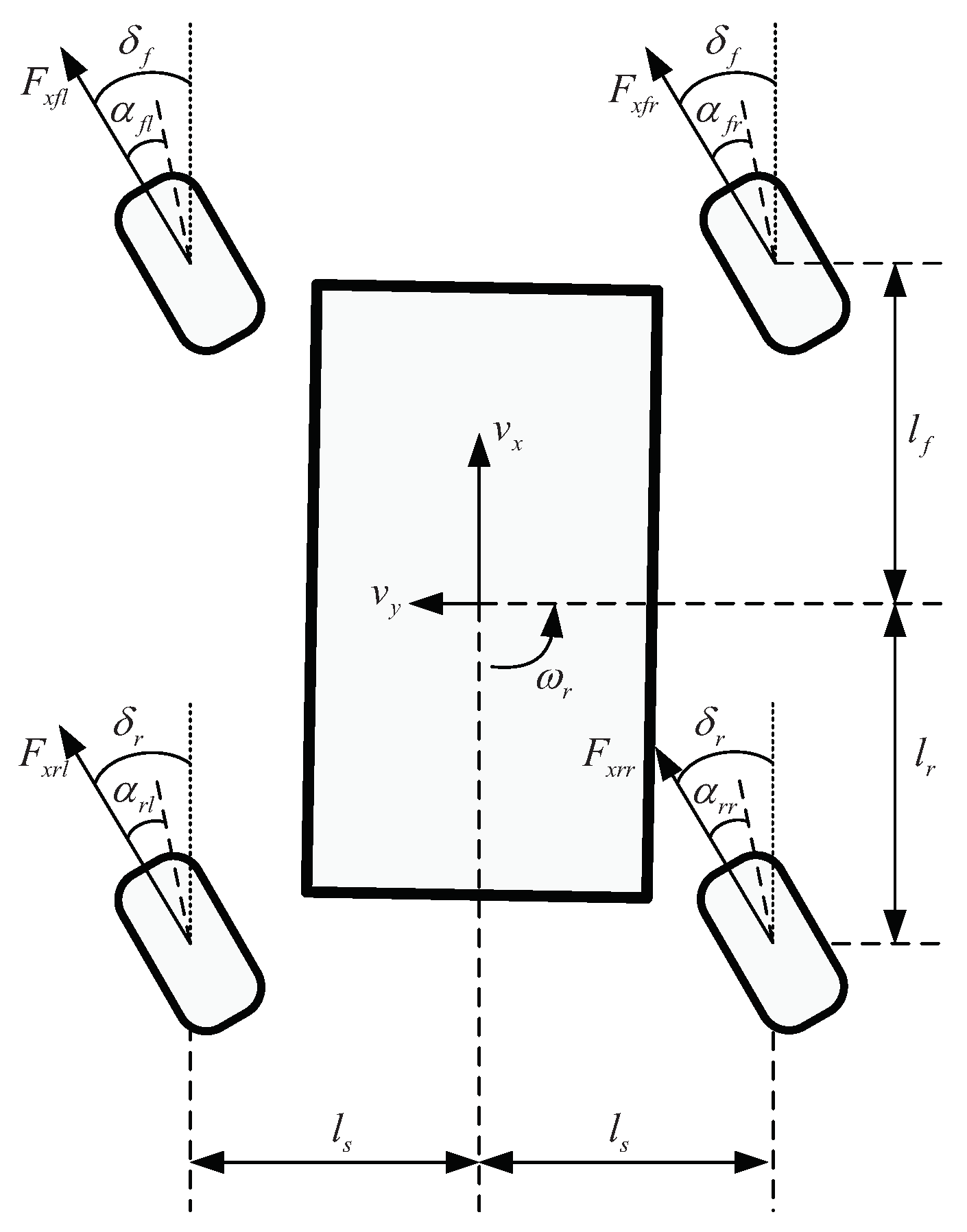
In this study, an electric vehicle with four-wheel steering and independent four-wheel drive is considered. The structure of the vehicle used for estimating the friction coefficient is shown in Figure 3. The vertical tire force and side-slip angle of each tire can be calculated using this model. In this figure, $l_f$ and $l_r$ represent the distances from the front and rear axles, respectively, to the center of gravity (CG). $l_s$ is equal to half of the front and rear wheel treads. $v_x$ and $v_y$ represent the longitudinal and lateral velocities, respectively, at the CG. ${\omega }_r$ is the yaw rate. The subscripts “$fl$”, “$fr$”, “$rl$”, and “$rr$” denote the values corresponding to the front left, front right, rear left, and rear right tires, respectively. $F_{xi}$ and ${\alpha }_i$ ($i=fl$, $fr$, $rl$, and $rr$) are the longitudinal tire force and side-slip angle, respectively, of the corresponding tire. ${\delta }_f$ and ${\delta }_r$ are the steering angles of the front and rear wheels, respectively.

2.1. Tire Force and Effective Radius Estimation

The estimated vertical load force on each tire can be expressed as [27,28,29]:

$$\left\{\begin{array}{c}{\widehat{F}}_{zfl}={\displaystyle \frac{mg{l}_r}{2L}}-{\displaystyle \frac{m{a}_x{h}_c}{2L}}-{\displaystyle \frac{m{a}_y{h}_c}{2l_s}}\\ {\widehat{F}}_{zfr}={\displaystyle \frac{mg{l}_r}{2L}}-{\displaystyle \frac{m{a}_x{h}_c}{2L}}+{\displaystyle \frac{m{a}_y{h}_c}{2l_s}}\\ {\widehat{F}}_{zrl}={\displaystyle \frac{mg{l}_f}{2L}}+{\displaystyle \frac{m{a}_x{h}_c}{2L}}-{\displaystyle \frac{m{a}_y{h}_c}{2l_s}}\\ {\widehat{F}}_{zrr}={\displaystyle \frac{mg{l}_f}{2L}}+{\displaystyle \frac{m{a}_x{h}_c}{2L}}+{\displaystyle \frac{m{a}_y{h}_c}{2l_s}}\end{array}\right.,$$

(1)

where $a_x$ and $a_y$ represent the longitudinal and lateral accelerations, respectively, at the CG, which can be obtained by means of integrated GPS/INS sensors [30]; $L=l_f+l_r$; $h_c$ and m are the height of the CG and the total mass, respectively; and g denotes the acceleration due to gravity.

Under normal conditions, the effective radius of each tire is mainly determined by the vertical force on that tire and can be estimated as [31]:

$${\widehat{R}}_{wi}=R_g-\frac{d_{ri}}{3},$$

(2)

where $i=fl$, $fr$, $rl$, and $rr$; ${\widehat{R}}_{wi}$ is the estimated effective radius of the corresponding tire; $R_g$ is the geometric radius of the tire; and $d_{ri}=\frac{{\widehat{F}}_{zi}}{k_z}$ is the deflection of the tire under the vertical force acting on it, where $k_z$ is the vertical stiffness of the tire.

Based on the dynamics of each wheel, the longitudinal force on each wheel can be estimated as:

$${\widehat{F}}_{xi}=\frac{T_i-J_w{\dot{\omega }}_i}{{\widehat{R}}_{wi}}+{\widehat{F}}_{zi}{f}_r,$$

(3)

where $i=fl$, $fr$, $rl$, and $rr$; $J_w$ and $f_r$ are the rotational inertia and rolling resistance coefficient, respectively, of each wheel, which are constant factors; and $T_i$ and ${\dot{\omega }}_i$ are the drive torque and angular acceleration, respectively, of the corresponding wheel. The drive torque can be obtained from the motor control system, and the angular acceleration can be obtained from the wheel angular acceleration sensors.

Due to the coupling of the lateral forces on the tires on the same axle, it is difficult to calculate the lateral force on each tire separately. However, the lateral forces on the front and rear axles can be estimated based on the vehicle dynamics [32]:

$$\left\{\begin{array}{c}\hfill {\widehat{F}}_{yf}=\frac{1}{l_f+l_r}(l_{f}m{a}_y-I_z{\dot{\omega }}_r)\\ \hfill {\widehat{F}}_{yr}=\frac{1}{l_f+l_r}(l_{r}m{a}_y-I_z{\dot{\omega }}_r)\end{array}\right.,$$

(4)

where ${\widehat{F}}_{yf}$ and ${\widehat{F}}_{yr}$ are the estimated lateral forces on the front and rear axles, respectively, and $I_z$ denotes the moment of inertia around the vertical axle.

2.2. Calculation of the Tire Side-Slip Angles and Slip Ratios

The speed and direction of each wheel can be calculated as follows [33,34,35,36,37]:

$$\left\{\begin{array}{c}{v}_{xfl}=\left(v_x-{\omega }_r{l}_s\right)cos{\delta }_f+\left(v_y+{\omega }_r{l}_f\right)sin{\delta }_f\\ v_{xfr}=\left(v_x+{\omega }_r{l}_s\right)cos{\delta }_f+\left(v_y+{\omega }_r{l}_f\right)sin{\delta }_f\\ v_{xrl}=\left(v_x-{\omega }_r{l}_s\right)cos{\delta }_r+\left(v_y-{\omega }_r{l}_r\right)sin{\delta }_r\\ v_{xrr}=\left(v_x+{\omega }_r{l}_s\right)cos{\delta }_r+\left(v_y-{\omega }_r{l}_r\right)sin{\delta }_r\end{array}\right.$$

(5)

and:

$$\left\{\begin{array}{c}{\theta }_{fl}=arctan\left(\frac{v_y+{\omega }_r{l}_f}{v_x-{\omega }_r{l}_s}\right)\\ {\theta }_{fr}=arctan\left(\frac{v_y+{\omega }_r{l}_f}{v_x+{\omega }_r{l}_s}\right)\\ {\theta }_{rl}=arctan\left(\frac{v_y-{\omega }_r{l}_r}{v_x-{\omega }_r{l}_s}\right)\\ {\theta }_{rr}=arctan\left(\frac{v_y-{\omega }_r{l}_r}{v_x+{\omega }_r{l}_s}\right)\end{array}\right.,$$

(6)

where $v_{xi}$ and ${\theta }_i$ ($i=fl$, $fr$, $rl$, and $rr$) are the speed and direction, respectively, of each wheel. The longitudinal speed, lateral speed, and yaw rate can be obtained by means of integrated GPS/INS sensors [30]. The front and rear steering angles can be obtained from angle sensors in the steering system.

The side-slip angle and slip ratio of each tire can be expressed as follows:

$${\alpha }_i=-{\delta }_i+{\theta }_i$$

(7)

and:

$$s_i=\frac{v_{xi}-{\omega }_i{\widehat{R}}_{wi}}{\max \left(v_{xi},{\omega }_i{\widehat{R}}_{wi}\right)},$$

(8)

where $i=fl$, $fr$, $rl$, and $rr$ and ${\omega }_i$ is the rolling speed of the corresponding wheel, which can be obtained from an angular speed sensor on that wheel.

2.3. Calculation of the Friction Coefficient

To obtain a reliable estimate of the friction coefficient, the characteristics of a tire are analyzed based on the Pacejka tire model [38], and the effectiveness of the corresponding friction coefficient estimation is discussed. Then, an optimization-based estimation algorithm is proposed.

2.3.1. Analysis of the Tire Model

The Magic tire model [38] is a commonly-used tire model in vehicle dynamics investigations, and it has also been found to be suitable for experimental applications. Thus, in this study, the Magic tire model is used to estimate the friction coefficient:

$$\left\{\begin{array}{cc}{F}_x& =D_{x}sin\left\{C_{s}arctan\left[B_{x}s-E_x\left(B_{x}s-arctan\left(B_{x}s\right)\right)\right]\right\}\hfill \\ F_y& =D_{y}sin\left\{C_{y}arctan\left[B_y\alpha -E\left(B_y\alpha -arctan\left(B_y\alpha \right)\right)\right]\right\}\hfill \end{array}\right.,$$

(9)

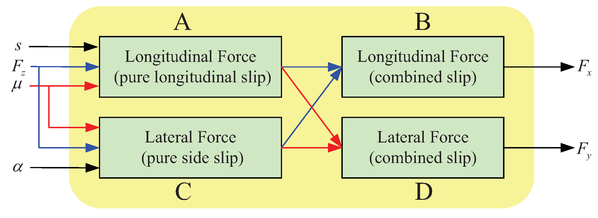
where $B_x$, $C_x$, $D_x$, $E_x$, $B_y$, $C_y$, $D_y$, and $E_y$ are the parameters of the tire model. The above functions constitute a common simplified description of the actual Magic tire model. The parameters of the tire model are mainly affected by the vertical force and the friction coefficient [38]. However, the friction coefficient does not explicitly appear in Equation (9), which makes this model difficult to use for friction coefficient estimation. The structure of the Magic tire model is visualized in Figure 4. This model consists of four parts [38], labeled from A–D. Parts A and C are used to calculate the longitudinal and lateral forces under conditions of pure longitudinal slip and pure side slip, respectively. Parts B and D are used to calculate the longitudinal and lateral forces, respectively, under combined slip conditions based on the calculation results from Parts A and C. The corresponding detailed calculations can be found in [38].

To facilitate the estimation of the friction coefficient, the Magic tire model can be further rewritten as follows:

$$\left\{\begin{array}{c}\hfill F_x={\mathrm{Magic}}_x\left(F_z,s,\alpha ,\mu \right)\\ \hfill F_y={\mathrm{Magic}}_y\left(F_z,s,\alpha ,\mu \right)\end{array}\right.,$$

(10)

where $F_x$ and $F_y$ are the longitudinal and lateral tire forces, respectively. The functions defined above provide a simple way to represent the Magic tire model for the purpose of friction coefficient estimation. The structures of these functions are visualized in Figure 5 and Figure 6, respectively.

For friction coefficient estimation, the vertical force, side-slip angle, and slip ratio are known and are viewed as parameters instead of inputs in the defined functions. Once the vertical force, side-slip angle, and slip ratio of a tire have been obtained, the relationships between $F_x$, $F_y$ and $\mu$ can be further rewritten as follows:

$$\left\{\begin{array}{c}\hfill F_x={\mathrm{Magic}}_{x,i}\left(\mu \right)\\ \hfill F_y={\mathrm{Magic}}_{y,i}\left(\mu \right)\end{array}\right.,$$

(11)

where $i=fl$, $fr$, $rl$, and $rr$ and the functions ${\mathrm{Magic}}_{x,i}$ and ${\mathrm{Magic}}_{y,i}$ represent the relationships between $F_x$, $F_y$, and $\mu$ when the vertical force, side-slip angle, and slip ratio are known for tire i. The structures of the functions defined above are illustrated in Figure 7 and Figure 8, respectively.

To facilitate the discussion of the estimation of the friction coefficient, the tire force use ratio is defined as follows:

$${\mu }_u=\frac{\sqrt{F_x^2+F_y^2}}{F_z}.$$

(12)

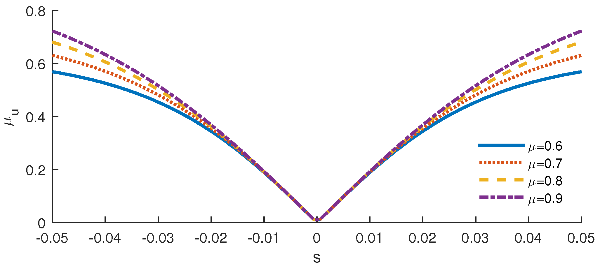
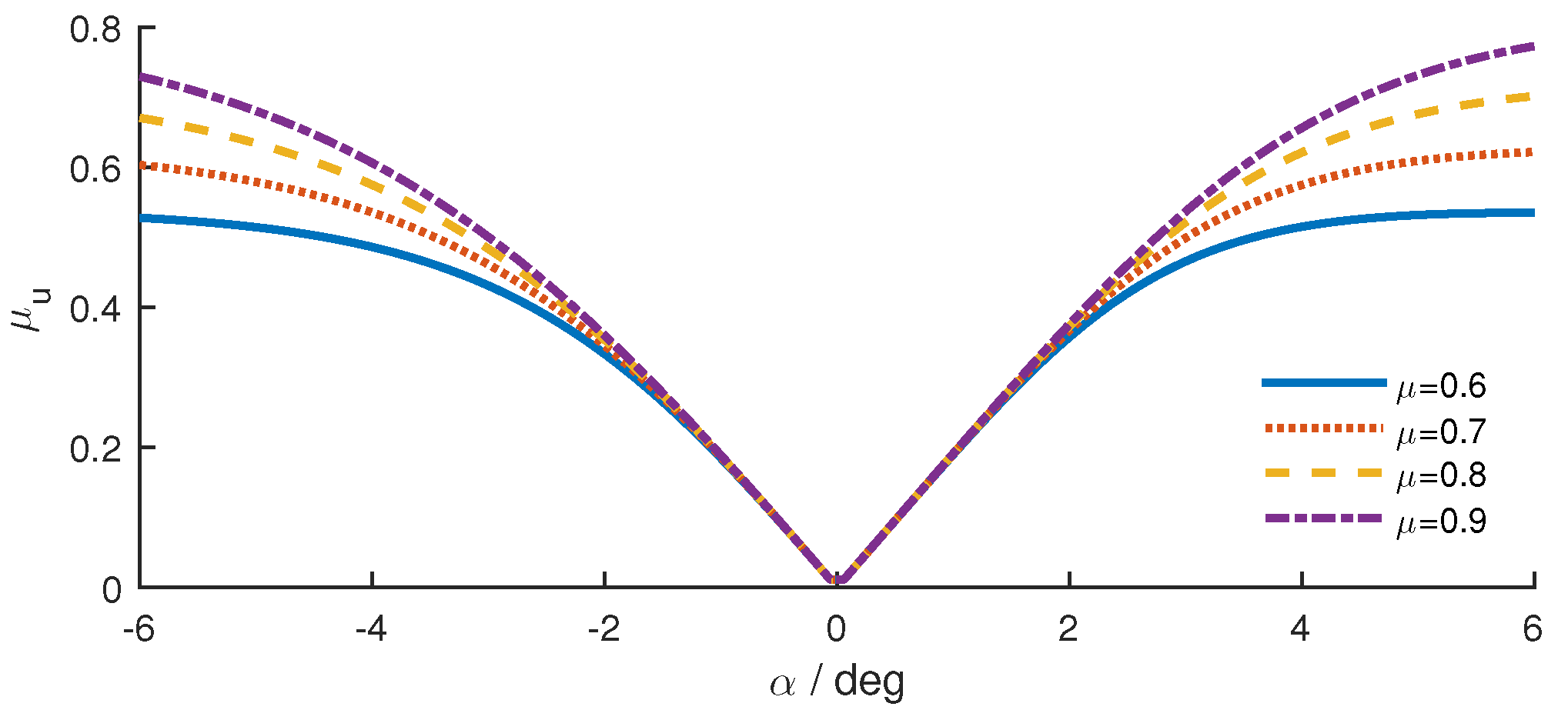
The relationships between the tire force use ratio and the slip ratio and side-slip angle with different friction coefficients are plotted in Figure 9 and Figure 10. Under conditions of a low slip ratio or low side-slip angle, the friction coefficient has only a small effect on the tire force use ratio, as shown in Figure 9. Thus, the friction coefficient also exerts only a small effect on the tire force under such conditions, which causes friction coefficient estimation based on the tire force to be unreliable. For instance, if the slip ratio and side-slip angle are both zero, then the longitudinal and lateral forces are also zero regardless of the friction coefficient. Indeed, the friction coefficient has no effect on the longitudinal and lateral forces under such conditions. Therefore, it is impossible to estimate the friction coefficient accurately based on the longitudinal and lateral tire forces under conditions of a low slip ratio and a low side-slip angle.

To measure the effectiveness of the estimation, an effectiveness factor is defined as follows:

$${\mu }_e=\frac{\sqrt{{\left({\mathrm{Magic}}_{x,i}\left(\mu +\Delta \mu \right)-{\mathrm{Magic}}_{x,i}\left(\mu \right)\right)}^2+{\left({\mathrm{Magic}}_{y,i}\left(\mu +\Delta \mu \right)-{\mathrm{Magic}}_{y,i}\left(\mu \right)\right)}^2}/F_z}{\Delta \mu },$$

(13)

where ${\mu }_e$ is the effectiveness factor, which indicates the effectiveness of the estimation, and ${\Delta }_{\mu }$ is a small number. ${\mu }_e$ can be viewed as reflecting the effect of the friction coefficient on the tire force use ratio. When ${\mu }_e$ is small, a change in the friction coefficient has only a small effect on the tire force, whereas a large value of ${\mu }_e$ indicates that this effect is large. Thus, friction coefficient estimation based on the tire force is inaccurate when ${\mu }_e$ is small. Because the estimated friction coefficients serve as the basis for speed planning, unreliable friction coefficient estimates should not be used. Only reliable estimates should be applied for speed planning.

2.3.2. Process of Estimation

To obtain a reliable estimate of the friction coefficient, the following estimation process is considered. The longitudinal tire force can be estimated from Equation (3), and the lateral force on each axle can be estimated from Equation (4). Because the lateral force on each axle is the total lateral force on both tires on the same axle, under ideal conditions, the following equations should be satisfied:

$$\left\{\begin{array}{c}{\mathrm{Magic}}_{x,fl}\left({\widehat{\mu }}_f\right)={\widehat{F}}_{xfl}\hfill \\ {\mathrm{Magic}}_{x,fr}\left({\widehat{\mu }}_f\right)={\widehat{F}}_{xfr}\hfill \end{array}\right.$$

(14)

and:

$${\mathrm{Magic}}_{y,fl}\left({\widehat{\mu }}_f\right)+{\mathrm{Magic}}_{y,fr}\left({\widehat{\mu }}_f\right)={\widehat{F}}_{yf}.$$

(15)

To facilitate the calculation, the following optimization problem is defined to estimate the friction coefficient of each front tire:

$$\begin{array}{cc}\hfill min:F_M\left({\widehat{\mu }}_f\right)=& w_x{({\mathrm{Magic}}_{x,fl}\left({\widehat{\mu }}_f\right)-{\widehat{F}}_{fl})}^2+w_x{({\mathrm{Magic}}_{x,fr}\left({\widehat{\mu }}_f\right)-{\widehat{F}}_{fr})}^2\hfill \\ \hfill \hspace{1em}& +w_y{({\mathrm{Magic}}_{y,fl}\left({\widehat{\mu }}_f\right)+{\mathrm{Magic}}_{y,fr}\left({\widehat{\mu }}_f\right)-{\widehat{F}}_{yf})}^2\hfill \end{array}$$

(16)

where ${\widehat{\mu }}_f$ is the estimated friction coefficient of each front tire. The meaning of Equation (16) is that if the estimated friction coefficient is equal to the actual value, then $F_M\left({\widehat{\mu }}_f\right)=0$. Thus, the friction coefficient of the tires on the front axle can be estimated by means of the optimization problem defined in Equation (16). The friction coefficient of the tires on the rear axle can also be estimated using the same method.

At each sampling instant, two estimated friction coefficients and their corresponding effectiveness factors can be obtained according to Equations (13) and (16). Due to the uncertainty of the model and the error in the numerical computations, the values from several successive sampling instants are used for estimation. The pseudocode for obtaining a reliable estimate of the friction coefficient is presented in Algorithm 1. In this algorithm, $n_t$ is the total number of sampling instants used for estimation in each sampling window, $m_e$ is the total number of effective estimates, ${\mu }_{eU}$ is the threshold for accepting an estimated friction coefficient as reliable, ${\mu }_{eL}$ is the threshold for accepting a friction coefficient estimate from a single sampling instant for use in the final estimation, and $\widehat{\mu }$ is the final output of the friction coefficient estimation process.

Algorithm 1 Friction coefficient estimation.

Input:${\mu }_{ei,j}$, ${\widehat{\mu }}_{i,j}$ ($i=f$ and r; $j=1,2,\cdots ,n_t$)

Output:$\widehat{\mu }$

1: procedure

2:   if $max({\mu }_{ef,1},{\mu }_{er,1})>{\mu }_{eU}$ then

3:     ${\widehat{\mu }}_s=0$

4:     $m_e=0$

5:     for $j=1\to n_t$ do

6:       for $i=f,r$ do

7:         if ${\mu }_{ei,j}>{\mu }_{eL}$ then

8:           ${\widehat{\mu }}_s={\widehat{\mu }}_s+{\widehat{\mu }}_{i,j}$

9:           $m_e=m_e+1$

10:         end if

11:       end for

12:     end for

13:     $\widehat{\mu }={\widehat{\mu }}_s/m_e$

14:     return $\widehat{\mu }$

15:   else

16:    A reliable estimate cannot be found in this sampling window.

17:   end if

18: end procedure

2.4. Torque Injection

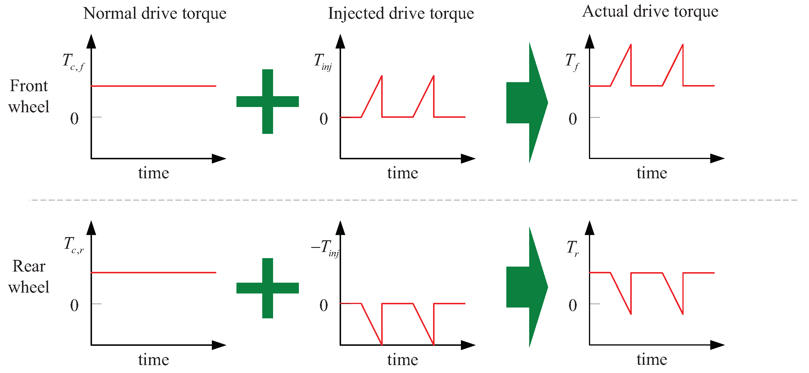
The relationship between the effectiveness factor and the tire slip ratio is illustrated in Figure 11. As shown in this figure, as the slip ratio increases, the effectiveness factor also increases. Thus, the friction coefficient estimation is more reliable with a higher slip ratio. By contrast, when a vehicle is traveling on a flat road at a constant speed, the tire slip ratio of each tire is low, which may lead to inaccurate estimation, as discussed previously. Thus, to obtain reliable estimates, the torque injection method is applied for friction coefficient estimation. The front wheels are injected with drive torques, and the rear wheels are injected with equal braking torques. The slip ratios of the front and rear wheels become larger as the injected torques increase. Thus, the estimation of the friction coefficient becomes more reliable as the slip ratio of each tire increases.

The torque injection method can be used to force tires to work at high slip ratios while having only a small effect on the longitudinal dynamics of the vehicle [25]. However, note that torque injection also leads to tire wear and power loss. Thus, the need for reliable estimation should be balanced with the disadvantages of torque injection. The principles of and procedure for the torque injection method are illustrated in Figure 12 and Figure 13, respectively. In these figures, $T_{c,f}$ and $T_{c,r}$ denote the normal front and rear drive torques, respectively, without torque injection; $F_{x,sum}$ denotes the resultant longitudinal drive force on the four tires; $T_{inj}$ is the injected drive torque; and $T_f$ and $T_r$ are the actual drive torques on the front and rear wheels, respectively. As indicated in Figure 12 and Figure 13, in the torque injection method, the front wheels are injected with drive torques, and the rear wheels are injected with equal braking torques. Thus, the total injected drive torque has no effect on the vehicle’s motion, but higher slip ratios of the front and rear wheels can be obtained, which are essential for accurately estimating the friction coefficient.

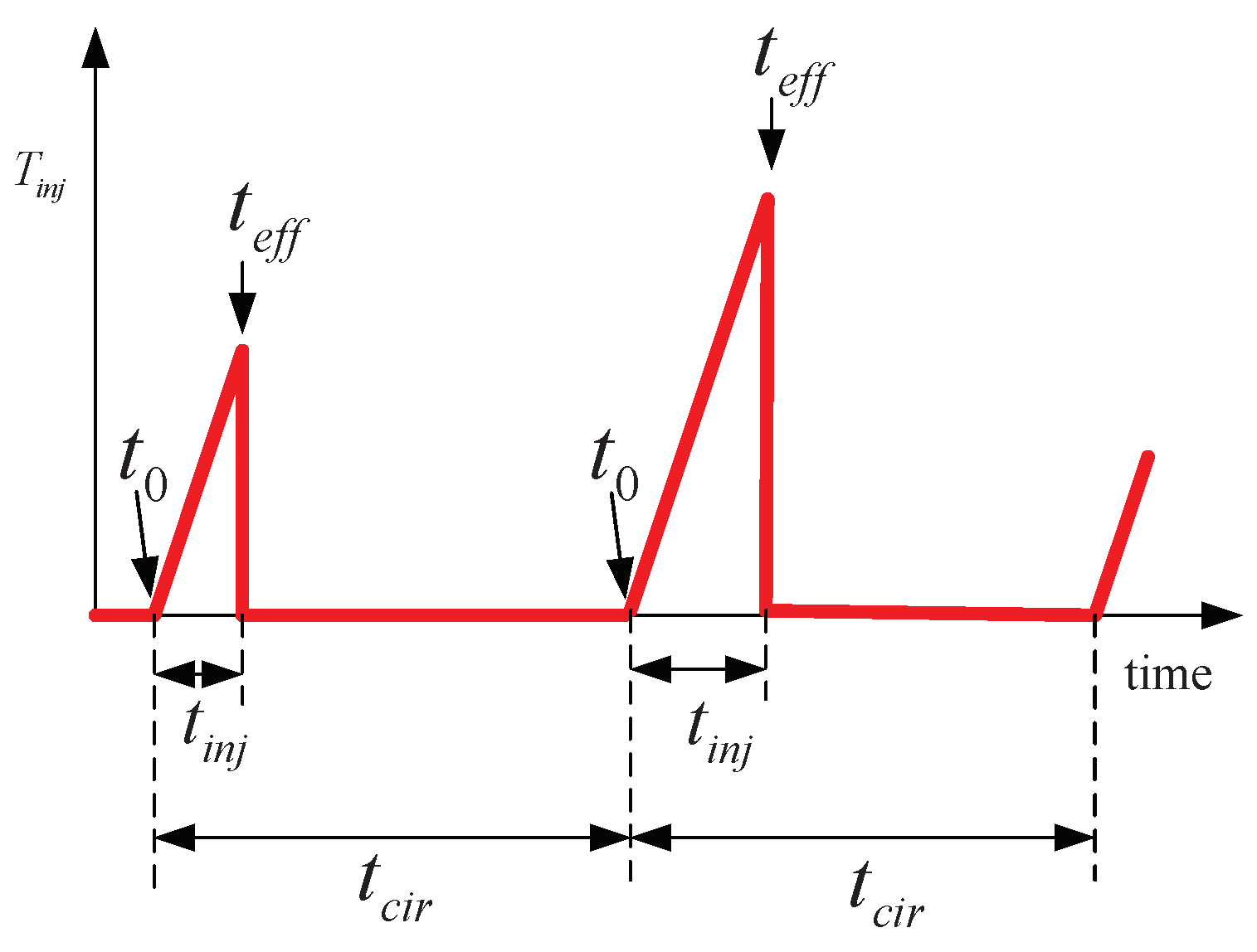
In this paper, an adaptive torque injection method is proposed for friction coefficient estimation. The torque injection signal is illustrated in Figure 14. In this figure, $t_{cyc}$ denotes the constant length of the torque injection cycle. A shorter cycle improves the update frequency for road friction estimation, but increases the power loss, and vice versa. $t_0$ denotes the start time of each cycle. $t_{eff}$ denotes the time when a reliable friction coefficient is obtained in each cycle.

The torque injected in each cycle is calculated as follows:

$$\left\{\begin{array}{c}{T}_{inj}=K_T·t_{inj}\hfill \\ t_{inj}=t-t_0\hfill \end{array}\right.,$$

(17)

where t is the current time, $T_{inj}$ is the injected torque, and $K_T$ is a constant parameter used to calculate $T_{inj}$. At the beginning of each cycle, the injected torque is zero.

As the injected torque increases, the slip ratios of the front and rear wheels also increase. Thus, the effectiveness factor will also increase. Once the effectiveness factor reaches the specified threshold, a reliable estimate of the friction coefficient can be obtained; the time at which this occurs is denoted by $t_{eff}$. The injected torque is then set to zero for the time remaining in the current cycle, as indicated in Figure 14. $t_{inj}$ and $T_{inj}$ may be different from one cycle to another. The torque injected into the front wheels is $T_{inj}$. The torque injected into the rear wheels is $-T_{inj}$.

3. Speed Planning

Generally, it is preferable to control a vehicle such that it moves at a constant desired speed for the purposes of comfort and economy. However, for a vehicle on a slippery road with a large curvature, traveling at a high speed may lead to a situation that could cause a serious traffic accident, such as lane departure. Thus, the vehicle’s speed should be planned online in accordance with the estimated friction coefficient and road shape.

In this section, an optimization-based algorithm for speed planning is proposed. First, the optimization variables, constraints, and objective function are designed for the speed planning task. Then, the optimization problem is constructed. Finally, a method of calculating the optimal safe speed is presented. Speed planning plays an important role in the vehicle control system, which serves as the link between the friction coefficient estimation and the motion controller.

3.1. Optimization Variables

To simplify the speed-planning problem, the path in front of the considered vehicle is separated into several segments of the same length by means of nodes. These segments and nodes are called path segments and path nodes for convenience. The speeds of the vehicle at each end of each of these segments are subjected to optimization. The travel speeds between the ends of each segment can be calculated through linear interpolation. For each segment, the path node at which the vehicle enters the segment is called the start node of the segment, and the path node at which the vehicle departs from the segment is called the end node of the segment. Note that a path can be separated into any number of segments for speed planning. However, the more segments are used for speed planning, the greater is the computational burden. Because the friction coefficient may change along the path, it is inappropriate to plan the entire path along the vehicle’s route simultaneously. To simplify the problem, the vehicle’s speed is planned successively for road sections of a certain length in front of the vehicle. As an example, the path in front of a vehicle is shown in Figure 15. The section of the path within a certain distance in front of the vehicle can be divided into n segments by $n+1$ nodes, as shown in Figure 16. These nodes are labeled from $p_0$–$p_n$. Note that $p_0$ is located at the CG of the vehicle. The path segment between $p_{i-1}$ and $p_i$ is denoted by $s_i$. Each of these path segments has a length of $l_p$.

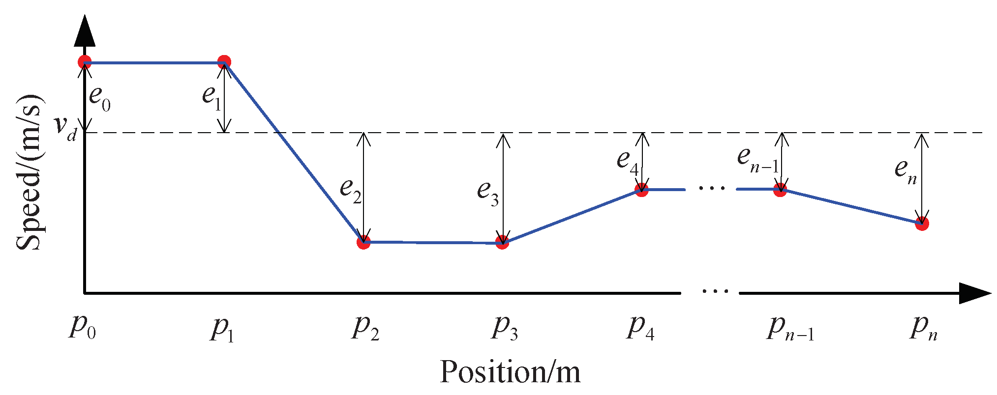
The planned speeds at $p_i$ ($i=1,2,\cdots ,n$) are represented by $v_i$ ($i=1,2,\cdots ,n$), respectively. Under the assumption that the speed of the vehicle varies linearly between each pair of adjacent nodes, the planned speeds of the vehicle along the path are further illustrated in Figure 17. As shown, once the planned speeds at these nodes have been determined, the planned speed profile along the path can be obtained. The error between the planned speed at each node and the desired speed is defined as:

$$e_i=v_i-v_d,$$

(18)

where $v_d$ is the desired speed. Clearly, if $e_i=0$ for all $i=1,2,\cdots ,n$, then the planned speed is equal to the desired speed along the entire path. Once $e_i$ ($i=1,2,\cdots ,n$) has been determined, $v_i$ ($i=1,2,\cdots ,n$) can be calculated as:

$$v_i=v_d+e_i.$$

(19)

As shown in Figure 18, the planned speeds can also be determined from the speed errors at the nodes. Thus, the speed errors at the nodes, denoted by $\mathit{e}={\left[\begin{array}{cccccc}{e}_0& e_1& e_2& \cdots & e_{n-1}& e_n\end{array}\right]}^T$, are defined as the decision variables for speed planning. Note that because the speed of the vehicle cannot track a step reference, the speed at node $p_0$ is not designated as one of the decision variables.

3.2. Constraints

This subsection presents the speed-planning constraints. First, constraints on the speed on a path segment are designed by considering several dangerous driving conditions. Then, constraints on the speed at a node are discussed. Finally, constraints for speed planning along the entire considered path are proposed.

3.2.1. Constraints on the Speed on a Path Segment

Consider the speed plan for a path segment. Traveling at an excessively high speed on the segment may lead to a skid or rollover. To avoid a skid, the lateral acceleration should satisfy:

$$a_y=\frac{v^2}{R_{min}}⩽\mu g,$$

(20)

where $R_{min}$ is the minimum radius of the path segment. Thus, a constraint on the planned speed as determined by the lateral acceleration can be defined as:

$$v_{Smax}=f_{sS}\sqrt{\mu g{R}_{min}},$$

(21)

where $f_{sS}<1$ is a safety factor for avoiding skid conditions.

To avoid rollover, the lateral acceleration should satisfy:

$$mg{l}_s⩾m{a}_y{h}_c=m\frac{v^2}{R_{min}}{h}_c.$$

(22)

The limit on the speed for avoiding rollover can thus be defined as:

$$v_{Rmax}=f_{sR}\sqrt{\frac{g{l}_s{R}_{min}}{h_c}},$$

(23)

where $f_{sR}<1$ is a safety factor for avoiding rollover conditions.

Thus, the maximum safe speed on a path segment can be expressed as:

$$v_{smax}=\min \left(v_{Smax},v_{Rmax}\right).$$

(24)

3.2.2. Constraints on the Speed at a Node

Generally, each node is adjacent to two path segments. To ensure safety, the maximum allowable planned speed at a node should be equal to the minimum value between the maximum safe speeds on the two adjacent segments, as expressed below:

$$v_{nmax,i}=\min \left(v_{smax,i},v_{smax,i+1}\right),$$

(25)

where $v_{smax,L}$ and $v_{smax,R}$ are the maximum safe speeds on the segments preceding and following the node, respectively. For the last node $p_n$, only the constraints on the path segment $s_n$ need to be considered.

Due to the limits of the road friction, the longitudinal acceleration should be limited to avoid tire slip. Because the lateral velocity of the vehicle is small, the derivative of the speed is simply used to approximate the longitudinal acceleration:

$$\left|{\dot{v}}_x\right|\approx \left|a_x\right|⩽f_{sL}·\mu ·g,$$

(26)

where $f_{sL}<1$ is a safety factor for limiting the longitudinal acceleration of the vehicle.

For a given path segment, the travel time of the vehicle on that segment is limited by the maximum safe speed on that segment; this limitation can be expressed as:

$$t_t<\frac{l_p}{v_{smax}}.$$

(27)

The planned speed profile along a segment is obtained through linear interpolation from the planned speeds at the end points. Thus, the derivative of the speed is constant in each segment. A constraint on the change in speed in a segment can be calculated as follows:

$$|v_e-v_s|⩽t_t·f_{sL}·\mu ·g,$$

(28)

where $v_s$ and $v_e$ are the planned vehicle speeds at the start and end points, respectively.

Equation (28) can be further rewritten as:

$$-v_{dec}⩽v_e-v_s⩽v_{dec},$$

(29)

where $v_{dec}=t_t{f}_{sL}·\mu ·g$.

3.2.3. Constraints on the Planned Speed Profile along the Path

In summary, according to Equations (26)–(29), the constraints on the planned speeds at all nodes can be expressed as:

$$\left\{\begin{array}{c}{v}_{min}⩽v_1⩽v_{nmax,1}\\ v_{min}⩽v_2⩽v_{nmax,2}\\ ⋮\\ v_{min}⩽v_n⩽v_{nmax,n}\end{array}\right.$$

(30)

and:

$$\left\{\begin{array}{c}-v_{dec1}⩽v_1-v_0⩽v_{dec1}\\ -v_{dec2}⩽v_2-v_1⩽v_{dec2}\\ ⋮\\ -v_{decn}⩽v_n-v_{n-1}⩽v_{decn}\end{array}\right..$$

(31)

By substituting Equation (19) into Equations (30) and (31), the speed-planning constraints can be rewritten as:

$$\left\{\begin{array}{c}{v}_{min}-v_d⩽e_1⩽v_{nmax,1}-v_d\\ v_{min}-v_d⩽e_2⩽v_{nmax,2}-v_d\\ ⋮\\ v_{min}-v_d⩽e_n⩽v_{nmax,n}-v_d\end{array}\right.$$

(32)

and:

$$\left\{\begin{array}{c}-v_{dec1}+e_0⩽e_1⩽v_{dec1}+e_0\\ -v_{dec2}⩽e_2-e_1⩽v_{dec2}\\ ⋮\\ -v_{decn}⩽e_n-e_{n-1}⩽v_{decn}\end{array}\right..$$

(33)

Equations (32) and (33) can be further rewritten as:

$$\left\{\begin{array}{c}{\mathbf{b}}_L⩽\mathbf{Ae}⩽{\mathbf{b}}_U\hfill \\ {\mathbf{b}}_{lb}⩽\mathbf{e}⩽{\mathbf{b}}_{ub}\hfill \end{array}\right.,$$

(34)

where $\mathit{e}=\left[\begin{array}{c}{e}_1\\ e_2\\ ⋮\\ e_n\end{array}\right]$, ${\mathit{b}}_L=\left[\begin{array}{c}{v}_{min}-v_d\\ v_{min}-v_d\\ ⋮\\ v_{min}-v_d\end{array}\right]$, ${\mathit{b}}_U=\left[\begin{array}{c}{v}_{nmax,1}-v_d\\ v_{nmax,2}-v_d\\ ⋮\\ v_{nmax,3}-v_d\end{array}\right]$, ${\mathit{b}}_{lb}=\left[\begin{array}{c}-v_{dec1}+e_0\\ -v_{dec2}\\ ⋮\\ -v_{decn}\end{array}\right]$, ${\mathit{b}}_{ub}=\left[\begin{array}{c}{v}_{dec1}+e_0\\ v_{dec2}\\ ⋮\\ v_{decn}\end{array}\right]$, and $\mathit{A}=\left[\begin{array}{cccccc}1& 0& 0& \cdots & 0& 0\\ -1& 1& 0& \cdots & 0& 0\\ 0& -1& 1& \cdots & 0& 0\\ ⋮& ⋮& ⋮& \ddots & ⋮& ⋮\\ 0& 0& 0& \cdots & 1& 0\\ 0& 0& 0& \cdots & -1& 1\end{array}\right]$.

3.3. Objective Function

To reduce the error between the desired and planned speeds, the following objective function is defined:

$$\mathrm{F}\left(\mathbf{e}\right)=\frac{1}{2}{\mathbf{e}}^T\mathbf{He},$$

(35)

where $\mathit{H}=\left[\begin{array}{ccccc}1& 0& 0& \cdots & 0\\ 0& 1& 0& \cdots & 0\\ 0& 0& 1& \cdots & 0\\ ⋮& ⋮& ⋮& \ddots & ⋮\\ 0& 0& 0& \cdots & 1\end{array}\right]$. The optimal planned speed can be obtained by minimizing $\mathrm{F}\left(\mathit{e}\right)$.

3.4. Construction of the Optimization Problem

Considering the discussed constraints, the optimization problem for planning the optimal safe speed profile is constructed as follows:

$$min:\mathrm{F}\left(\mathbf{e}\right)$$

(36)

subject to:

$$\left\{\begin{array}{c}{\mathbf{b}}_L⩽\mathbf{Ae}⩽{\mathbf{b}}_U\hfill \\ {\mathbf{b}}_{lb}⩽\mathbf{e}⩽{\mathbf{b}}_{ub}\hfill \end{array}\right..$$

(37)

The optimization problem defined above is a typical quadratic programming problem, which can be solved with qpOASES [39]. By solving this optimization problem, the speed errors at all nodes can be obtained. The planned speed at each node along the path can then be calculated in accordance with Equation (19). Using the conventional linear interpolation method, the planned speed profile on each segment along the path can also be obtained.

3.5. Calculation of the Planned Speed

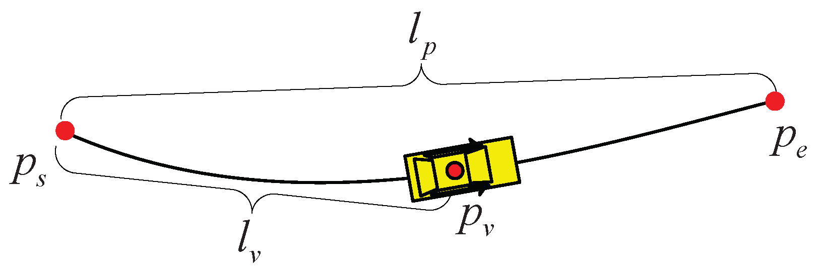
Once the optimal speed planning solution has been found, the planned speed at any point can be calculated through simple linear interpolation. Consider a path section with a single segment, as shown in Figure 19. $p_s$ and $p_e$ are the start and end points, respectively, of this segment. $p_v$ is the position of the vehicle. $l_v$ is the length of the path between $p_s$ and $p_v$. $s_s$ is the length of the path between $p_s$ and $p_e$. The planned speed of the vehicle at $p_v$ can be calculated as:

$$v_p=\frac{l_v}{l_p}{v}_s+\frac{l_p-l_v}{l_p}{v}_e,$$

(38)

where $v_s$ and $v_e$ are the planned speeds at $p_s$ and $p_e$, respectively.

4. Numerical Simulation

To verify the effectiveness of the proposed ISPFCE algorithm, a numerical simulation was conducted with CarSim and Simulink. The vehicle model in CarSim is a 27-degree-of-freedom full-vehicle model that is equipped with nonlinear tire models. The measurement noise characteristics of realistic sensors (such as those in the RT4000 navigation system from Oxford Technical Solutions Ltd., Bicester, U.K.) were reproduced in the simulation. The proposed algorithm was implemented using Simulink. The simulation parameters are listed in

Table 1. Simulation parameters.

Parameter	Value	Parameter	Value
m	1412 kg	$R_g$	0.3 m
$l_f$	1.016 m	$l_r$	1.564 m
$l_s$	0.77 m	$h_c$	0.54 m

.

In the simulation, the initial speed of the vehicle at the origin point, which was also considered to be the desired speed, was set to 23 m/s. The shape and curvature of the road path are shown in Figure 20 and Figure 21, respectively. The minimum radius of the path was 187.5 m ($1/R=$ 0.0053(1/m)), as shown in Figure 21. The friction coefficient was initially 0.85; subsequently, it decreased to 0.2 and then returned to 0.85 in a stepwise manner, as shown in Figure 21.

As discussed previously, the proposed ISPFCE algorithm can be applied in combination with previously-investigated motion controllers. In the simulation, two motion controllers were designed for comparison, one based on fuzzy model predictive control [12] (Controller A) and one based on a linear quadratic regulator [40] (Controller B). The performances of these motion controllers with and without the proposed ISPFCE algorithm are presented for comparison.

The lane-keeping performance and speeds of vehicles controlled by Controllers A and B with and without ISPFCE are illustrated in Figure 22, Figure 23 and Figure 24. As shown in Figure 23, without the proposed ISPFCE algorithm, Controllers A and B attempt to control the corresponding vehicles such that they travel at the desired speed along the entire road. However, as discussed above, due to the limited road friction at a tight bend, it is impossible for the vehicles to pass through the bend at the desired speed. Figure 22 indicates that the vehicles controlled by Controllers A and B cannot remain on the path at the bend, meaning that the vehicles cannot stay within their lane on the road. The large lateral position errors shown in Figure 24 indicate that the vehicles leave the road during the simulation.

By contrast, with the proposed ISPFCE algorithm, the speeds of the vehicles controlled by Controllers A and B are reduced to low values before the tight bend with the corresponding low friction coefficient, as indicated in Figure 23. Thus, these vehicles can move along the reference path with small tracking errors, as shown in Figure 22 and Figure 24. This comparison demonstrates that the proposed ISPFCE algorithm can be applied with different motion controllers to handle roads with changes in their friction coefficients. Notably, traveling at a low speed at all times would lead to increased time consumption and decreased traffic flow. Thus, once a high friction coefficient is again detected, the vehicle speed should be increased. As shown in Figure 23, the vehicle speeds return to the desired value once a high friction coefficient is again detected, demonstrating that the proposed ISPFCE algorithm can handle various changes in the friction coefficient on a curved road.

The control inputs to the vehicles controlled by Controllers A and B with ISPFCE are shown in Figure 25 and Figure 26. The details of the friction estimation and speed planning are further plotted in Figure 27, Figure 28, Figure 29, Figure 30, Figure 31, Figure 32, Figure 33 and Figure 34. As shown in Figure 21, the road friction coefficient changes from 0.85 to 0.2 at approximately 550 m and changes back to 0.85 at approximately 2900 m. Due to the time elapsed during each torque injection cycle, there is some delay before the estimated friction coefficient reaches the real value, as illustrated in Figure 28. The results of online speed planning are presented in Figure 29. As shown in Figure 31, the initial speed plan is Plan A. Because the estimated friction coefficient is high, the ISPFCE algorithm assumes that the vehicle can move at the desired high speed along the path. Once a decrease in the friction coefficient is detected, the ISPFCE algorithm determines that the desired high speed is not safe on the curved road. Thus, speed Plan B is generated, as shown in Figure 30. The relationship between speed Plan B and the road curvature is plotted in Figure 32. As shown in Figure 32, the planned vehicle speed is reduced to a low value before the tight bend. Thus, the vehicle can follow the path safely. While the vehicle is still on a section of the road with low friction, it should follow the path at a low speed. Thus, speed Plan C is generated. As shown in Figure 33, the planned speed is very low on these low-friction bends. When a high friction coefficient is again detected, the ISPFCE algorithm determines that it is safe for the vehicle to again move along the reference path at the desired speed. Thus, speed Plan D is generated, as plotted in Figure 34, in which the planned speed is increased to the desired value to satisfy the set requirements.

These simulation results demonstrate that the proposed ISPFCE algorithm can handle changes in the friction coefficient on a curved road. Once a decrease in the friction coefficient that may lead to dangerous conditions is detected, a low, safe vehicle speed can be planned to pass through the tightly-curved road section. When the friction coefficient again increases to a high value, the ISPFCE algorithm can plan a return to the desired speed along the road. Moreover, these simulation results also demonstrate the flexibility of using the ISPFCE algorithm in combination with different motion controllers for general applications.

5. Conclusions

In this paper, an integrated speed-planning and friction coefficient estimation (ISPFCE) algorithm is proposed. The friction coefficient is estimated online by means of torque injection. If a decrease in the friction coefficient is detected before a tight bend, the speed can be adjusted to a safe value before an accident could potentially occur. A simulation based on CarSim and Simulink demonstrates the effectiveness of the proposed algorithm. The present paper reveals that a sudden decrease in the friction coefficient is dangerous for vehicles on curved roads, potentially leading to serious traffic accidents. Conventional lane-keeping systems and cruise control systems without friction estimation may fail to handle such a decrease in the friction coefficient properly, particularly on a curved road with a large curvature. One feasible solution is to estimate the friction coefficient online and reduce the speed before such a bend with a low friction coefficient, which is the key purpose of the algorithm proposed in this paper.

As discussed above, speed-planning and friction coefficient estimation are critical for ensuring the safety of vehicles. In the proposed ISPFCE algorithm, only speed planning for the host vehicle is considered. In fact, however, it is also useful to estimate the friction coefficients and planned safe speeds for other vehicles. Thus, given a suitable vehicular network, it is also essential to send relevant information to other vehicles that cannot estimate the friction coefficient for planning safe speeds. The question of how to use the information collected by the host vehicle to improve the safety of other nearby vehicles will be investigated in the future. Due to the practical limitations concerning available equipment and experimental sites, only a numerical simulation is reported in this study. Further experimental investigations will also be conducted to improve the performance of the ISPFCE algorithm.

References

1. D’Ambrosio, C.; Sbarra, G.; Tiberti, M.; Verrelli, C.M.; Consolini, L. A new spatial learning control for autonomous vehicles: Experimental results. In Proceedings of the Annual Conference on System of Systems Engineering, Paris, France, 19–22 June 2018; pp. 68–73. [Google Scholar]
2. Antonelli, D.; Pasquale, L.; Salvatore, A.; Tiberti, M.; Verrelli, C.M. Electric vehicles under slip constraints: Experimental results. In Proceedings of the AEIT International Annual Conference, Bari, Italy, 3–5 October 2018; pp. 1–6. [Google Scholar]
3. Marino, R.; Pasquale, L.; Scalzi, S.; Verrelli, C.M. Automatic Rotor Speed Reference Generator for Electric Vehicles Under Slip Constraints. IEEE Trans. Intell. Transp. Syst. 2015, 16, 3473–3478. [Google Scholar] [CrossRef]
4. Sc., A.E.D.; Arem, B.V.; Amditis, A.; Lytrivis, P.; Portouli, E.; Papp, Z.; Schutter, B.D.; Ploeg, J.; Baskar, L.D.; Naus, G. Handbook of Intelligent Vehicles; Springer: Berlin, Germany, 2012; pp. 1217–1267. [Google Scholar]
5. Wang, J.; Rajamani, R. Should adaptive cruise-control systems be designed to maintain a constant time gap between vehicles? IEEE Trans. Veh. Technol. 2004, 53, 1480–1490. [Google Scholar] [CrossRef]
6. Qu, T.; Chen, H.; Cao, D.; Guo, H. Switching-based stochastic model predictive control approach for modeling driver steering skill. IEEE Trans. Intell. Transp. Syst. 2015, 16, 365–375. [Google Scholar] [CrossRef]
7. Marino, R.; Scalzi, S.; Netto, M. Nested PID steering control for lane keeping in autonomous vehicles. Control Eng. Pract. 2011, 19, 1459–1467. [Google Scholar] [CrossRef]
8. Tagne, G.; Talj, R.; Charara, A. Higher-Order Sliding Mode Control for Lateral Dynamics of Autonomous Vehicles, with Experimental Validation. In Proceedings of the Intelligent Vehicles Symposium, Gold Coast, QLD, Australia, 23–26 June 2013; pp. 678–683. [Google Scholar]
9. Yang, J.; Zhao, J.; Lei, J. Research on three kinds of lane keeping method based on anti-saturation and adaptive method. Int. J. Hybrid Inf. Technol. 2015, 8, 317–326. [Google Scholar] [CrossRef]
10. Lei, J.; Wu, H.; Yang, J.; Zhao, J. Sliding mode lane keeping control based on separation of translation and rotation movement. Opt. Int. J. Light Electron Opt. 2016, 127, 4369–4374. [Google Scholar] [CrossRef]
11. Raksincharoensak, P.; Nagai, M.; Shino, M. Lane keeping control strategy with direct yaw moment control input by considering dynamics of electric vehicle. Veh. Syst. Dyn. 2006, 44, 192–201. [Google Scholar] [CrossRef]
12. Bian, C.; Yin, G.; Zhang, N.; Xu, L. Takagi-sugeno fuzzy model predictive controller design for combining lane keeping and speed tracking of four wheels steering and four wheels drive electric vehicle. In Proceedings of the Chinese Control and Decision Conference, Chongqing, China, 28–30 May 2017; pp. 4067–4072. [Google Scholar]
13. Luo, Y.; Chen, T.; Li, K. Nonlinear model predictive cruise control of hybrid electric vehicle. Chin. J. Mech. Eng. 2015, 51, 11–21. [Google Scholar] [CrossRef]
14. Wang, J.; Xu, X.; Liu, D.; Sun, Z.; Chen, Q. Self-learning cruise control using kernel-based least squares policy iteration. IEEE Trans. Control Syst. Technol. 2014, 22, 1078–1087. [Google Scholar] [CrossRef]
15. Taymans, A.; Melchior, P.; Malti, R.; Aioun, F.; Guillemard, F.; Servel, A. Cruise control of an electric vehicle through fractional linear feedforward prefiltering of an acceleration reference signal. IFAC-PapersOnLine 2017, 50, 12569–12574. [Google Scholar] [CrossRef]
16. Schwickart, T.; Voos, H.; Hadji-Minaglou, J.R.; Darouach, M.; Rosich, A. Design and simulation of a real-time implementable energy-efficient model-predictive cruise controller for electric vehicles. J. Frankl. Inst.-Eng. Appl. Math. 2015, 352, 603–625. [Google Scholar] [CrossRef]
17. Eichelberger, A.H.; McCartt, A.T. Toyota drivers’ experiences with dynamic radar cruise control, pre-collision system, and lane-keeping assist. J. Saf. Res. 2016, 56, 67–73. [Google Scholar] [CrossRef] [PubMed]
18. Morand, A.; Moreau, X.; Melchior, P.; Moze, M.; Guillemard, F. CRONE cruise control system. IEEE Trans. Veh. Technol. 2016, 65, 15–28. [Google Scholar] [CrossRef]
19. Reichhartinger, M.; Horn, M. Robust cascaded automatic cruise control of electric vehicles. Int. J. Robust Nonlinear Control 2016, 26, 662–680. [Google Scholar] [CrossRef]
20. Qiu, C.; Liu, C.; Shen, F.; Chen, J. Design of automobile cruise control system based on Matlab and fuzzy PID. Trans. Chin. Soc. Agric. Eng. 2012, 28, 197–202. [Google Scholar]
21. Lee, Y.; Ryoo, Y.J. Design of cruise control system for electric vehicle using piece-wised control. Adv. Intell. Syst. Comput. 2014, 269, 37–44. [Google Scholar] [CrossRef]
22. Onieva, E.; Godoy, J.; Villagra, J.; Milanes, V.; Perez, J. On-line learning of a fuzzy controller for a precise vehicle cruise control system. Expert Syst. Appl. 2013, 40, 1046–1053. [Google Scholar] [CrossRef] [Green Version]
23. Consolini, L.; Verrelli, C.M. Learning control in spatial coordinates for the path-following of autonomous vehicles. Automatica 2014, 50, 1867–1874. [Google Scholar] [CrossRef]
24. Marino, R.; Scalzi, S.; Verrelli, C.M. Speed and traction control in electric vehicles with induction motors. In Proceedings of the Electrical Systems for Aircraft, Railway and Ship Propulsion, Bologna, Italy, 16–18 October 2012. [Google Scholar]
25. Chen, Y.; Wang, J. Adaptive vehicle speed control with input injections for longitudinal motion independent road frictional condition estimation. IEEE Trans. Veh. Technol. 2011, 60, 839–848. [Google Scholar] [CrossRef]
26. Deur, J.; Pavković, D.; Burgio, G.; Hrovat, D. A model-based traction control strategy non-reliant on wheel slip information. Veh. Syst. Dyn. 2011, 49, 1245–1265. [Google Scholar] [CrossRef]
27. Xiong, L.; Yu, Z.; Wang, Y.; Yang, C.; Meng, Y. Vehicle dynamics control of four in-wheel motor drive electric vehicle using gain scheduling based on tyre cornering stiffness estimation. Veh. Syst. Dyn. 2012, 50, 831–846. [Google Scholar] [CrossRef]
28. Zhenta, L. Optimal allocation of tire force based on vehicle stability. J. Mech. Electr. Eng. 2015, 32, 433–438. [Google Scholar] [CrossRef]
29. Osborn, R. TaehyunShim. Independent control of all-wheel-drive torque distribution. Veh. Syst. Dyn. 2006, 44, 529–546. [Google Scholar] [CrossRef]
30. Zhang, H.; Huang, X.; Wang, J.; Karimi, H.R. Robust energy-to-peak sideslip angle estimation with applications to ground vehicles. Mechatronics 2015, 30, 338–347. [Google Scholar] [CrossRef]
31. Jazar, R.N. Vehicle Dynamics: Theory and Application; Springer: Berlin, Germany, 2008. [Google Scholar]
32. Villagra, J.; D’Andréanovel, B.; Fliess, M.; Mounier, H. A diagnosis-based approach for tire-road forces and maximum friction estimation. Control Eng. Pract. 2011, 19, 174–184. [Google Scholar] [CrossRef]
33. Wang, J.; Longoria, R.G. Coordinated vehicle dynamics control with control distribution. In Proceedings of the American Control Conference, Minneapolis, MN, USA, 14–16 June 2006; pp. 5348–5353. [Google Scholar]
34. Bian, C.; Yin, G.; Hu, M.; Ning, Z.; Nan, C. Fault tolerant control design for all wheels independent drive and steering electric vehicle with singular effective drive wheel. In Proceedings of the Vehicle Power & Propulsion Conference, Hangzhou, China, 17–20 October 2016. [Google Scholar]
35. Guvenc, B.; Acarman, T.; Guvenc, L. Coordination of steering and individual wheel braking actuated vehicle yaw stability control. In Proceedings of the IEEE Intelligent Vehicles Symposium, Columbus, OH, USA, 9–11 June 2003; pp. 288–293. [Google Scholar]
36. Wang, R.; Wang, J. Fault-tolerant control for electric ground vehicles with independently-actuated in-wheel motors. J. Dyn. Syst. Meas. Control Trans. ASME 2012, 134, 021014. [Google Scholar] [CrossRef]
37. Feiqiang, L.; Jun, W.; Zhaodu, L. On the vehicle stability control for electric vehicle based on control allocation. In Proceedings of the IEEE Vehicle Power and Propulsion Conference, Harbin, China, 3–5 September 2008; pp. 1–6. [Google Scholar]
38. Pacejka, H.B. Tire and Vehicle Dynamics, 2nd ed.; Elsevier: New York, NY, USA, 2006. [Google Scholar]
39. Ferreau, H.J.; Kirches, C.; Potschka, A.; Bock, H.G.; Diehl, M. qpOASES: A parametric active-set algorithm for quadratic programming. Math. Program. Comput. 2014, 6, 327–363. [Google Scholar] [CrossRef]
40. Tavan, N.; Tavan, M.; Hosseini, R.; Tavan, N.; Tavan, M.; Hosseini, R. An optimal integrated longitudinal and lateral dynamic controller development for vehicle path tracking. Lat. Am. J. Solids Struct. 2014, 12, 1006–1023. [Google Scholar] [CrossRef]
Figure 1. Structure of a vehicle system including the proposed algorithm.
Algorithms 12 00044 g001
Figure 2. Structure of the friction coefficient estimation algorithm.
Algorithms 12 00044 g002
Figure 3. Vehicle structure model used for estimation.
Algorithms 12 00044 g003
Figure 4. Structure of the Magic tire model.
Algorithms 12 00044 g004
Figure 5. Structure of the Magic x function.
Algorithms 12 00044 g005
Figure 6. Structure of the Magic y function.
Algorithms 12 00044 g006
Figure 7. Structure of the Magic x , i function.
Algorithms 12 00044 g007
Figure 8. Structure of the Magic y , i function.
Algorithms 12 00044 g008
Figure 9. Tire force use ratio as a function of the slip ratio.
Algorithms 12 00044 g009
Figure 10. Tire force use ratio as a function of the side-slip angle.
Algorithms 12 00044 g010
Figure 11. Effectiveness factor as a function of the tire slip ratio for different friction coefficients.
Algorithms 12 00044 g011
Figure 12. Principles of torque injection.
Algorithms 12 00044 g012
Figure 13. Procedure for torque injection.
Algorithms 12 00044 g013
Figure 14. Sawtooth torque injection signal.
Algorithms 12 00044 g014
Figure 15. An example path.
Algorithms 12 00044 g015
Figure 16. Division of the example path.
Algorithms 12 00044 g016
Figure 17. Speeds at nodes.
Algorithms 12 00044 g017
Figure 18. Speed errors at nodes.
Algorithms 12 00044 g018
Figure 19. A path segment.
Algorithms 12 00044 g019
Figure 20. Road path.
Algorithms 12 00044 g020
Figure 21. Curvature and friction coefficient of the road.
Algorithms 12 00044 g021
Figure 22. Lane-keeping performance of vehicles controlled by different controllers: (a) Controller A and (b) Controller B.
Algorithms 12 00044 g022
Figure 23. Speeds of vehicles controlled by different controllers: (a) Controller A and (b) Controller B.
Algorithms 12 00044 g023
Figure 24. Path tracking errors: (a) Controller A and (b) Controller B.
Algorithms 12 00044 g024
Figure 25. Steering angles of vehicles controlled by different controllers: (a) Controller A + ISPFCE and (b) Controller B + ISPFCE.
Algorithms 12 00044 g025
Figure 26. Drive torques of vehicles controlled by different controllers: (a) Controller A + ISPFCE and (b) Controller B + ISPFCE.
Algorithms 12 00044 g026
Figure 27. Injected drive torques: (a) Controller A + ISPFCE and (b) Controller B + ISPFCE.
Algorithms 12 00044 g027
Figure 28. Estimated friction coefficients: (a) Controller A + ISPFCE and (b) Controller B + ISPFCE.
Algorithms 12 00044 g028
Figure 29. Speed plans: (a) Controller A + ISPFCE and (b) Controller B + ISPFCE.
Algorithms 12 00044 g029
Figure 30. Piecewise speed plans: (a) Controller A + ISPFCE and (b) Controller B + ISPFCE.
Algorithms 12 00044 g030
Figure 31. Speed Plan A: (a) Controller A + ISPFCE and (b) Controller B + ISPFCE.
Algorithms 12 00044 g031
Figure 32. Speed Plan B: (a) Controller A + ISPFCE and (b) Controller B + ISPFCE.
Algorithms 12 00044 g032
Figure 33. Speed Plan C: (a) Controller A + ISPFCE and (b) Controller B + ISPFCE.
Algorithms 12 00044 g033
Figure 34. Speed Plan D: (a) Controller A + ISPFCE and (b) Controller B + ISPFCE.
Algorithms 12 00044 g034