Computation of Compact Distributions of Discrete Elements

Abstract

In our daily lives, many plane patterns can actually be regarded as a compact distribution of a number of elements with certain shapes, like the classic pattern mosaic. In order to synthesize this kind of pattern, the basic problem is, with given graphics elements with certain shapes, to distribute a large number of these elements within a plane region in a possibly random and compact way. It is not easy to achieve this because it not only involves complicated adjacency calculations, but also is closely related to the shape of the elements. This paper attempts to propose an approach that can effectively and quickly synthesize compact distributions of elements of a variety of shapes. The primary idea is that with the seed points and distribution region given as premise, the generation of the Centroidal Voronoi Tesselation (CVT) of this region by iterative relaxation and the CVT will partition the distribution area into small regions of Voronoi, with each region representing the space of an element, to achieve a compact distribution of all the elements. In the generation process of Voronoi diagram, we adopt various distance metrics to control the shape of the generated Voronoi regions, and finally achieve the compact element distributions of different shapes. Additionally, approaches are introduced to control the sizes and directions of the Voronoi regions to generate element distributions with size and direction variations during the Voronoi diagram generation process to enrich the effect of compact element distributions. Moreover, to increase the synthesis efficiency, the time-consuming Voronoi diagram generation process was converted into a graphical rendering process, thus increasing the speed of the synthesis process. This paper is an exploration of elements compact distribution and also carries application value in the fields like mosaic pattern synthesis.

1. Introduction

The synthesis of texture patterns has been an important research subject. Traditional texture synthesis technologies are mainly designed for raster textures, which record texture information only in the form of raster images and have no explicit records or expressions of the geometric content expressed in the textures (such as basic units composing the textures and unit distribution information). Gradually, a number of texture patterns have been found to be distributions of numerous discrete elements. If images are described as geometric distributions of many vector elements, a better effect of pattern synthesis will be achieved from the aspect of element distribution. On this basis, many researchers have begun studying the topics of discrete element distribution [1,2,3,4,5,6,7,8,9], among which the synthesis of compact element distributions is the most challenging. Compact element distributions need to arrange one or several given types of elements in a random and possibly compact way (as show in Figure 1, the compact distribution effects of square and circular elements). This process calls for not only the attention to the element location distributions, but also judgment of the crashing and overlapping relations between elements, which are closely connected with the shapes of the elements. Therefore, it has been a difficult task to synthesize compact element distributions. Currently, the majority of the research is focused on discrete element distributions. Although some researchers, such as Ijiri [10] and Liu [5], have achieved relatively compact element distributions, their methods require both the construction of complicate relations between elements and algorithms with high computational complexity.

Other researchers have studied compact element distributions from the aspect of space division, among which the Voronoi diagram is the most frequently used. The Voronoi diagram is a plane partitioning method based on distance, which can effectively achieve small-region partitioning. Some researchers utilized the Voronoi diagram to partition the space to achieve the compact distribution of small-region elements [11,12,13]. Other studies [11,12,13] adopted L₂-metric as a distance measurement, thus making the shape of the small regions defined as approximately hexagonal. Hausner et al. [14] tried to use the Manhattan distance to measure the distance in the Voronoi diagram, thereby generating a partition of regions similar to square shapes. However, in the practical application, like mosaic pattern synthesis, compact distributions of elements in various shapes will be frequently needed. Drawing from this, we modify the distance metric to affect the shape of the Voronoi region remarkably, thus generating partition of Voronoi region in various shapes. This paper attempts to adopt four distance metrics to realize several types of region partitions, such as those composed of rectangles, circles, ovals, and triangles, and to further achieve compact element distributions of many shapes.

Compared with traditional methods, our method is characterized by the following advantages:

(1) Compact distributions of elements of various shapes were achieved. By adopting different distance metrics of the Voronoi diagram, the shapes of the generated Voronoi regions can be controlled, thus realizing compact distributions of elements of various shapes, such as rectangles, circles, triangles, and ovals.

(2) Our method is highly efficient. By converting the Voronoi generation process into a graphical rendering process, the GPU (Graphics Processing Unit) parallel computing ability can be fully utilized for calculation, and thus the synthesis speed can reach interactive efficiency.

(3) The pattern synthesis can be controlled. By adjusting parameters, users are able to control the size and distribution direction of elements and further control the pattern synthesis to satisfy various synthesis requirements.

This paper not only conducts discussion on geometric topic of compact element distributions, but also achieves the generation of synthesis results with special artistic beauty, which carries practical significance in fields such as pattern design and artistic creation.

2. Related Work

In the field of computer graphics, a number of researchers have studied compact distributions, and a series of approaches have been proposed. In the following part of this paper, these approaches will be introduced in three categories, namely, physics-based simulation, sample-based synthesis, and process-based modeling. Because the work in this paper is closely related with the Voronoi diagram, a brief introduction of work on the Voronoi diagram is presented in the last part of this chapter.

Physics-based simulation. During physics-based simulation, the compact distribution of the discrete elements will be regarded as a piling process of physical elements. The discrete elements will be arranged tightly in space according to the laws of dynamics, such as collision, contact, and friction, and some manually defined rules.

Cho et al. [15] utilized a physics-based simulation method and managed to accumulate a certain number of randomly initialized elements in a rectangular box by gravity and friction. Researchers such as Guendelman [16] adopted a dual representation to express nonconvex-shaped elements to effectively deal with the collision and contact during element aggregation, and succeeded in generating realistic dynamic distributions of discrete elements.

Using a physics-based simulation method, users can visually control the modeling results. However, they need to be fully aware of the modeling objects and algorithm application and must also be able to repeatedly test the input parameters based on experience. Therefore, this approach is labor-intensive and time-consuming. Moreover, this method calls for a large amount of data calculation, consequently leading to low operational efficiency.

Sample-based synthesis. During sample-based synthesis, given a small region of an element distribution as a sample, users synthesize a larger-scale element distribution that has a similar pattern to the sample. This method develops from sample-based synthesis, mainly on raster textures in the early stage. Starting from synthesizing by pixel [8,9], later synthesizing by patch [17,18] is introduced with better efficiency and performance, followed by many methods on textures synthesis like image analogies [19]. Although these methods could synthesize patterns with large-scale elements distribution based on sample image, they merely deal with raster information with no explicit record or expression of the geometric information in the textures (information like basic element of the textures or distributions of elements), thus often resulting in poor performance when synthesizing patterns with compact element distributions.

Afterwards, research began on the synthesis of distribution relationship of geometric elements in texture patterns. The key point is to construct local position relationship between elements and overall distribution rules of these elements based on the samples. Some researchers referred to local neighborhood matching in texture synthesis for the synthesis process [1,2,10,14,20,21] and attempted to guarantee the local distribution characteristics of the synthesized elements. Barla et al. [20] used Delaunay triangulation to construct the neighborhood relationship between elements and then replaced the seed points one by one based on this relationship. Ijiri et al. [10] used the same Delaunay method, but they adopted a local growing method for the distribution synthesis. Xu et al. [2] proposed a new approach to constructing the neighborhood relationship using a histogram to count the element distributions of a certain element type within a circle neighborhood to describe the neighborhood features of this element. Other researchers performed the synthesis based on the statistical features of the entire element distributions and sought to synthesize data with features similar to those of the samples. Barla et al. [3] calculated quantities such as the distance, angle, separation, and superposition between all the elements in the sample pattern and calculated their averages, variances, and Gaussian distributions. During synthesis, distributions of the peak points will gradually accord with the statistical features of the sample data via constant iteration. Other researchers, such as Hurtut [4], calculated the probability density function of elements of all types and synthesized the element distribution based on the calculation results. Some other researchers considered the statistical and local features of the entire set. Ma [1] extended the local neighborhood matching to an overall energy function optimization process, while Liu et al. [5], in addition to proposing a neighborhood coding method to describe the element neighborhood features, considered the overall features, such as the density and minimum distance, of all kinds of elements.

Sample-based methods have proven to be efficient in synthesizing discrete elements. However, when elements are closely arranged, a number of problems will occur due to the neglect of collision and overlapping situations between elements. If we take the collision and overlapping situations into consideration, the amount of calculation will be significantly increased.

Process-based modeling. In the process-based methods for element distribution simulation, finding the element distributions is regarded as a random sampling or an overall optimization process.

Many methods have been adopted to generate different element space distributions, among which the Poisson disk distribution is the most popular. This distribution can ensure that the elements are as evenly arranged as possible, while the distance between any two elements is not less than a user-defined threshold value. The two most classic algorithms to generate Poisson disk distributions are the dart-throwing algorithm [6] and Lloyd’s method [14]. Lloyd’s method, via progressive optimization in a certain region, constructs the Voronoi diagram to create point distributions. Then, the entire region is partitioned into small regions by every Voronoi region. On this basis, if these polygons have similar shapes to those of the discrete elements, the elements can be closely arranged by simply putting them into these polygons.

Voronoi diagram. The Voronoi diagram is a kind of fundamental data structure of space proximity relations [22]. On the basis of point set P of a plane, this diagram can divide this plane into Voronoi regions in the shape of a convex polygon. Every point p_i in the P corresponds a region V_i, making the distance between any point in V_i and p_i shorter than that between any point in V_i and p_j (j≠i). When generating the Voronoi diagram, various Voronoi region shapes can be achieved by adopting different distance metrics. Normally, the L_p-metrics is the most commonly used (also known as Minkowski distance) [23].

When p = 2 (that is, L₂-metrics), the shapes of Voronoi regions generated will approach a regular hexagon. When p = 1 (also known as Manhattan distance), the shapes will be the square rotated 45 degrees. Hausner et al. [14] attempted to adopt this function for compact distribution of square-shaped elements.

Apart from L_p-metrics, other functions like convex polygon-offset distance function [24] and the Moscow metric [25] are also introduced by researchers. There are also related works on the anisotropic Voronoi synthesis [26]. Moreover, the definition of the Voronoi diagram has been extended from two dimensions to three or more dimensions. The Voronoi diagram over curved surfaces [27,28] has also been researched. Some researchers even conducted work on the Voronoi diagram in non-Euclidean space metrics (like Riemannian geometry metric) [29,30].

This paper is mainly on how to achieve the compact distributions of elements in various shapes in plane space. L_p-metrics, as one of the most commonly used functions in Euclidean space and the most efficient way to generate the Voronoi diagram, has naturally become our key point. Besides L₁-metric and L₂-metric, we also try to achieve distributions of square-shaped elements by L_∞-metric, and distributions of elements in rectangular and oval shape by axial scale. Additionally, the triangle equidistant line method (regarded as a kind of convex polygon-offset distance function) is also adopted to generate compact distributions of triangle-shaped elements.

3. Methods of This Paper

3.1. Voronoi Diagram Based on Several Distance Metrics

In this paper, the calculation process of the centroidal Voronoi diagram is adopted for the Voronoi diagram generation with the following calculation process. First, generate the Voronoi diagram of N non-overlapping seed points in a plane, which partitions this plane into N regions with all the points in each region closer to the corresponding seed points than to other seed points, as shown in Figure 2a, Then, move the seed point of each region to the centroid of the corresponding region and generate the Voronoi diagram of the seed points again, and repeat the above process. According to the centroidal Voronoi diagram, the distribution of seed points will become increasingly balanced. Normally, the Voronoi region of a set of evenly distributed points will be similar to a relatively regular shape (as shown in Figure 2b).

In the most classical Voronoi diagram, L_p-metric is used to measure the distance between the p₀$\left(x_0,y_0\right)$ and p₁$\left(x_1,y_1\right)$ and among all the L_p-metrics, L₂-metric is the most commonly used.

$$\mathrm{d}({\mathrm{p}}_0,{\mathrm{p}}_1)=\sqrt{{\left(x_1-x_0\right)}^2+{\left(y_1-y_0\right)}^2}$$

With this metric, the generated Voronoi region is close to a regular hexagon (as shown in Figure 3a). Hausner et al. [8] used the L₁-metric (Manhattan distance).

$$\mathrm{d}({\mathrm{p}}_0,{\mathrm{p}}_1)=\left|x_1-x_0\right|+\left|y_1-y_0\right|$$

The polygons of the generated Voronoi diagram were close to square. To obtain Voronoi regions with more shapes, we attempt to adopt more metrics. Four additional distance metrics are introduced, which are Chebyshev distance, Chebyshev distance with axial scale, L₂-metric distance with axial scale, and equidistant line distance, and finally, distributions of squares, rectangles, ovals, and triangles are achieved, respectively. In the following part of this paper, the different metrics will be discussed in detail.

3.1.1. Chebyshev Distance

The Chebyshev distance defines the distance between two points $\left(x_1,y_1\right)$ and $\left(x_0,y_0\right)$ as $\max \left(\left|x_1-x_0\right|,\left|y_1-y_0\right|\right)$. It is not difficult to prove that it is equivalent to the L_p-metric with p→∞. The Voronoi region generated with this distance is the same shape, namely square, as the one generated with Manhattan metrics (as shown in Figure 3c). However, the differences between these two metrics are the directions of the coordinate axes. The axes of the Manhattan distance are inclined 45 degrees, while the axes of the Chebyshev distance are horizontal and vertical (as shown in Figure 4). In this paper, we use the Chebyshev distance because its axial directions conform with normal image space, which is easier to scale and control.

As shown in Figure 4, the side of the square is defined as L_a, while the diagonal line is defined as L_b; the axis xy corresponding to the Manhattan distance is shown in Figure 4a. The distance between any point $A\left(x_1,y_1\right)$ on the square side and the origin $O\left(x_0,y_0\right)$ is $\left|x_1-x_0\right|+\left|y_1-y_0\right|$, which is the sum of the red segment and blue segment in Figure 4a, that is, L_b /2. The axis xy corresponding to the Chebyshev distance is shown in Figure 4b. The distance between any point $A\left(x_1,y_1\right)$ on the square side and the origin $O\left(x_0,y_0\right)$ is $max\left(\left|x_1-x_0\right|,\left|y_1-y_0\right|\right)$, which is the length of the longer segment among the red and blue segments in the picture, La /2.

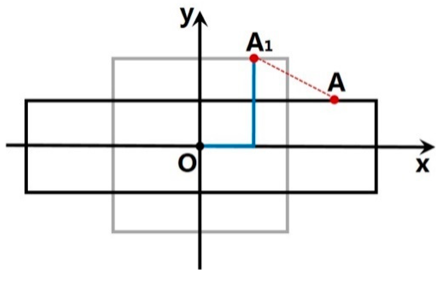
3.1.2. Chebyshev Distance with Axial Scale

The Chebyshev distance between p₀$\left(x_0,y_0\right)$ and p₁$\left(x_1,y_1\right)$ with axial scale is as follows:

$$\mathrm{d}({\mathrm{p}}_0,{\mathrm{p}}_1)=max\left(\beta \left|x_1-x_0\right|,\left(1/\beta \right)\left|y_1-y_0\right|\right).$$

With this metric, a rectangle-shaped Voronoi diagram is generated (as shown in Figure 3d). To obtain the Chebyshev distance with axial scale, the original Chebyshev space is scaled along two axial directions; as a result, the unit distance has been changed and the original square-shaped Voronoi diagram becomes a rectangle-shaped one.

As shown in Figure 5, let $\beta$ be 1/2 and the length of each square side be L_a before the axial scaling. For the rectangle after the scaling, the length is 2 × L_a, while the width is 1/2L_a. The distance from any point $A\left(x_1,y_1\right)$ on the rectangle to the origin point $O\left(x_0,y_0\right)$ is $max\left(\beta \left|x_1-x_0\right|,\left(1/\beta \right)\left|y_1-y_0\right|\right).$ To measure this distance, a correspondence between points A and point $A_1\left(\beta x_1,\left(1/\beta \right)y_1\right)$ on the square is defined, and the distance between point $A_1$ and the origin point is calculated based on the original Chebyshev space. Hence, the distance from any point $A\left(x_1,y_1\right)$ on the rectangle to the origin point $O\left(x_0,y_0\right)$ is L_a/2.

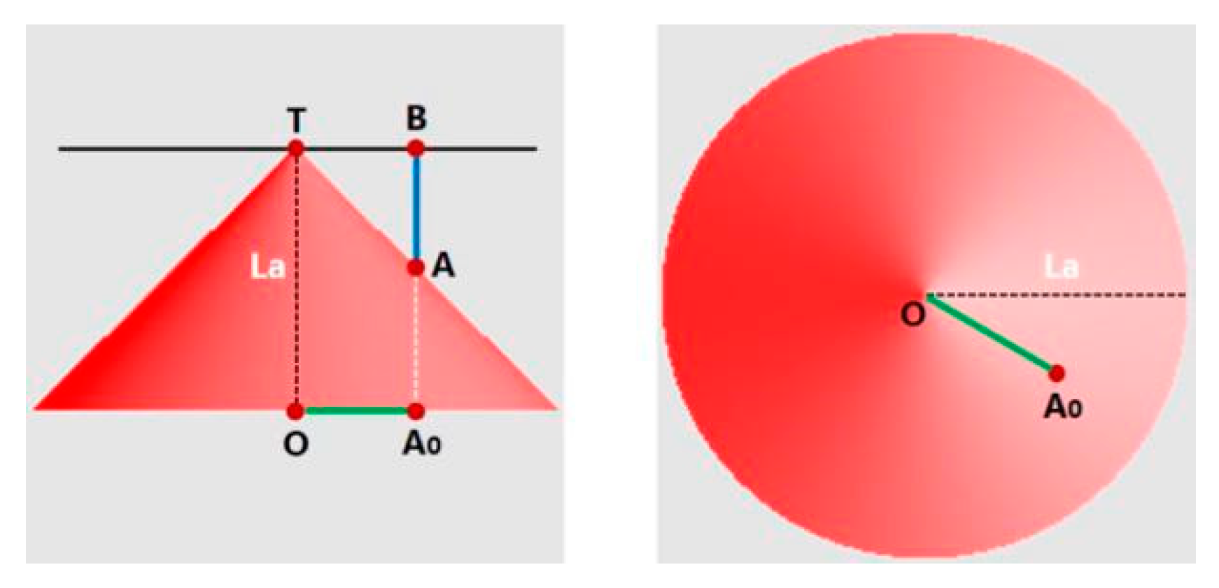
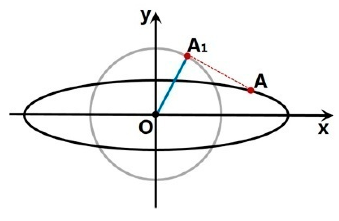
3.1.3. L₂-Metric Distance with Axial Scale

L₂-metric with axial scale can be expressed as follows:

$$\mathrm{d}({\mathrm{p}}_0,{\mathrm{p}}_1)=\sqrt{{\beta }^2{\left(x_1-x_0\right)}^2+{\left(1/\beta \right)}^2{\left(y_1-y_0\right)}^2}.$$

With this metric, the generated Voronoi region is close to an oval shape (as shown in Figure 6). In the same manner as the Chebyshev distance with axial scale mentioned above, for the L₂-metric distance with axial scale, the original Euclidean space is scaled along two axial directions; as a result, the unit distance is changed and the original circle-shaped Voronoi diagram becomes an oval-shaped one.

As shown in Figure 6, let $\beta$ be $1/2$ and the radius of the circle be $r$. With the transverse length of the oval defined as 4 × r after the axial scaling and the minor-axis length of the oval as r, the distance between any point $A\left(x_1,y_1\right)$ on the oval and the origin point $O\left(x_0,y_0\right)$ equals that between the point $A_1$ and origin point $O\left(x_0,y_0\right)$. $A_1$ is the corresponding point of $A$ on the circle, whose coordinates are $x_1$ and $y_1$ multiplied by the factors $\beta$ and $\left(\frac{1}{\beta }\right)$ respectively. This means that the distance between any point on the oval and the origin point $O\left(x_0,y_0\right)$ is r.

3.1.4. Equidistant Line Distance

The equidistant line distance is a kind of metric adopted in the paper to generate regular triangular regions. On the basis of this metric, the distance between two points is measured by the equidistant line of a regular triangle. The direction of the regular triangle in the space is defined as shown in Figure 7. Given a regular triangle with a side length of L_a, with the origin position defined as the center of gravity, draw a similar regular triangle within the original regular triangle with the centers of gravity of all the triangles at the origin point, and then the distance between any point on the triangle side and the origin point is defined as the distance between the center of gravity and the triangle vertex. When measuring the distance between $P\left(x_1,y_1\right)$ and $Q\left(x_0,y_0\right)$ with this metric, we need to define the origin point as P, construct regular triangles with P as the gravity center, and let the point Q be located on the side of the regular triangle. Hence, the distance between P and the vertex of the triangle is the same as that between P and Q.

The distance between any point $A\left(x_1,y_1\right)$ on the triangle and the origin point $O\left(x_0,y_0\right)$ is $\sqrt{3}/3La.$ However, instead of being a strict triangle, the final Voronoi region obtained with this metric is a dodecagon that is close to a triangle (as shown in Figure 7, right). The reason is that triangles with consistent directions cannot fill the entire plane with no gaps or overlaps. Therefore, during the repeating iteration process, the triangle is turned into the shape shown in Figure 7, left. Finding an approach to obtain a more accurate triangular region partition will be our future research direction.

3.2. Voronoi Diagram Generation Based on GPU Acceleration

To generate a Voronoi diagram, the iteration process must be repeated and every iteration process needs to loop through all the distribution points, which is quite time-consuming. Hoff et al. [30] proposed a method of converting the Voronoi generation process into a graphical rendering process. First, the distribution of the initial points is determined, and then a circular cone with height equal to the radius is constructed at each initial point location. The vertices of the cones are used as the initial seed points. The cones are the same in terms of all parameters except color. In this way, the height of the side part of the cone can be adopted to measure the distance from the corresponding points on the bottom surface to the center; thus, the correct Voronoi diagram can be obtained by rendering all the cones with visibility detection via the z-buffer algorithm. The Voronoi generation process is successfully transformed into a graphical rendering process, and the GPU parallel computing ability can be fully utilized to increase the speed. This paper, taking this as a reference, implemented a GPU rendering process to achieve quick generation of Voronoi regions with many shapes. In the following part of this paper, the Voronoi regions generated by GPU rendering are described—they are of five shapes; namely, circle, square, rectangle, oval, and triangle.

The key to accomplishing the Voronoi generation via geometric rendering and visibility detection with the z-buffer algorithm is to ensure that the height of any point on the side of the geometric shape is equal to the distance between the corresponding points of the random point on the bottom surface and the center. Taking the cone shown in Figure 8 as an example, the height of the cone and the radius of the bottom surface are both L_a, and the corresponding point of any random point A on the side is $A_0$. Given that the distance between $A_0$ and center is the yellow segment $\left|O{A}_0\right|$ and the height of A is the blue segment $\left|AB\right|$, based on $\left|TB\right|=\left|AB\right|$ and $\left|TB\right|=\left|O{A}_0\right|$, we conclude that $\left|AB\right|=\left|O{A}_0\right|$. As shown in Figure 9, by rendering a mass of three-dimensional cones, we can obtain the Voronoi diagram. In the rendering, the orthographic projection is adopted, and the z-buffer method is used for visibility detection.

To generate Voronoi diagrams in many shapes, we adopt many kinds of geometries that conform to the above distance conditions; the detailed information is shown in

Table 1. Shapes and sizes of geometries corresponding to different distance metrics.

Geometry		Distance Metric	Bottom Size	Height
Circular cone		Euclidean distance	Radius = La	La
Square pyramid		Manhattan distance	Side length = La	$\frac{\sqrt{2}}{2}La$
Square pyramid		Chebyshev distance	Side length = La	$\frac{1}{2}La$
Pyramid		Chebyshev distance with axial scale	Length = $\frac{1}{\beta }La$, width = $\beta La$	La
Elliptic cone		Euclidean distance with axial scale	axis = $\frac{1}{2\beta }La$, minor axis $=\frac{\beta }{2}La$	La
Triangular pyramid		Equidistant line distance	Side = La	$\frac{\sqrt{3}}{3}La$

.

Calculation process:

Step 1. Randomly generate initial distribution point set p.

Step 2. Show geometries (circular cone, square pyramid, pyramid, elliptic cone, and triangular pyramid) in different colors at every p(x, y) location; different colors can make it easier to distinguish different Voronoi regions.

Step 3. Rotate the geometry ψ(x, y) according to the direction field of p(x, y).

Step 4. Perform the depth measurement, and read the current drawing results; calculate the center of gravity of each Voronoi region; the results are the new distribution point set p.

Step 5. Repeat steps 2 to 4 for the new point set p until the specified number of iterations is reached.

Step 6. Place the elements at the locations of the final centers of gravity.

3.3. Parametric Control of Element Distribution

To make the synthesis output more variable and controllable, this paper introduces several approaches to control the size and direction of the generated Voronoi regions, thus achieving compact element distributions of changeable size and direction.

3.3.1. Changing of Element Sizes

Our research results indicate that the distribution of the initial point set has a significant effect on the synthesis results. A region with a more compact distribution of initial points usually eventually results in a smaller Voronoi region. Therefore, we propose to control the sizes of the Voronoi polygons by adjusting the parameters while generating the initial points to control the density. However, the experimental results show that if we only use the method described above to control the size, there will be situations in which the size gradually varies in the junctions of large and small polygons. This will create irregular polygons at the boundary (as shown in Figure 11a), which is not desirable. For this reason, in addition to controlling the density of the initial points, we utilize the method of changing the size of the geometry that was adopted during the synthesis process for better results.

Let $\alpha$ be the slope of the geometry used during the synthesis process, and take the circular cone in Figure 10 as an example. While generating the Voronoi region, use geometry with a smaller size (geometry with a larger $\alpha$) when a smaller region needs to be obtained and geometry with a larger size (geometry with a smaller $\alpha$) in other regions. Together with the initial point distribution in this region, better results can be achieved by changing the sizes of the elements (as shown in Figure 11b).

3.3.2. Changing of the Vector Field

During the iterative optimization process of generating the centroidal Voronoi diagram, the method in this paper can adjust the direction of the generated Voronoi region, which is shown in Step 3 of the calculation process in Chapter 3.2. Users can define a vector field ψ for the distribution region. Let the direction of the vector field of seed point p(x,y) be ψ(x,y). By rotating the geometry at p(x,y) to the direction ψ(x,y), we can obtain element distribution results by conforming to the vector field. Figure 12a is the vector field and Figure 12b is the generated Voronoi diagram based on the Chebyshev distance metric.

3.4. Placement of the Elements

Through the above methods, compact distributions of Voronoi regions with different shapes can be obtained. In order to realize the compact distributions of the discrete elements, we need to place the elements into every Voronoi region. However, because the Voronoi regions have different sizes and directions, the sizes and directions of the elements need to be adjusted while putting them into the regions to obtain the distribution results. Taking the size adjustment as an example, as shown in Figure 13, we need to extract the contour of every Voronoi region and adjust the size and direction based on the contour information.

4. Results

We use C++ programming to realize the algorithm and, based on OpenGL, the Voronoi diagram is successfully generated through three-dimensional graphical rendering.

4.1. Experimental Results

The pictures shown in Figure 14 are synthesis results that were obtained using the methods proposed in this paper. Figure 14a–d show distribution effects of squares, rectangles, ellipses, and triangles, respectively. Figure 14e,f show the compact distribution effects with elements varying from sizes and directions.

In particular, if random points are distributed throughout an image and the image information is used as a constraint, our algorithm can simulate the mosaic effect based on the image features, which means for any picture specified by the user, our algorithm can automatically convert the image into a mosaic-style image and obtain more artistic mosaic effects. As shown in Figure 16, Figure 17, Figure 18 and Figure 19 below, the mosaic effects are synthesized based on the image features.

4.2. Synthesis Effect Comparison

This paper conducts research on the compact distributions of discrete elements. The more compact the distribution is in a certain region, the higher the regional coverage scale. Therefore, the synthesis effect could be evaluated by the regional coverage scale. Methods of FritzscheL, P. [12], Smith, K. [26] and Hu, W. [13] are adopted to compare the synthesis effects from the following three aspects: synthesis result, coverage scale, and time consumption. The synthesis results of the method introduced in this paper are closely related to the number of iterations used to generate the centroidal Voronoi diagram.

Table 2. Comparison among different methods.

	Effect Picture	Average Coverage Scale	Average Time
Fritzsche L P		64.8%	1 min
K. Smith		68.1%	1 min
Hu W		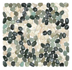84.3%	10 min
Author		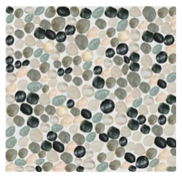85.6%	19 s

shows the results after 20 iterations. On the basis of the data in Table 2, the method of this paper is characterized by a larger coverage scale, lower time consumption, and a better synthesis result.

5. Discussion

This paper, by adopting a variety of distance metrics to generate Voronoi diagrams for compact distributions of Voronoi regions of many shapes, has finally achieved the compact distributions of elements of various shapes. During the synthesis process, by converting the time-consuming Voronoi diagram generation process into a graphical rendering process, the computational speed of the algorithm has been increased with the parallel computing ability of the GPU, thereby satisfying the interactive synthesis efficiency. Meanwhile, the methods in this paper can control the sizes and directions of the distribution elements to achieve synthesis results with a variation effect, thus enhancing the expressive effect of the synthesis results.

The methods proposed in this paper also have some limitations: (1) the generated Voronoi regions cannot exactly match the element’s shape, causing some gaps between elements or overlapping, which affects the synthesis results; (2) the distributions of elements of triangle shape are not perfect, because every triangle has three gaps on each side; (3) apart from the existing shapes, the possibility of obtaining Voronoi diagrams with other shapes, even general shapes, is a topic that is worthy of further research and discussion.

References

- Cho, J.H.; Xenakis, A.; Gronsky, S. Course 6: Anyone can cook: inside Ratatouille’s kitchen. In Proceedings of the SIGGRAPH ‘07 ACM SIGGRAPH 2007 courses, San Diego, CA, USA, 5–9 August 2007; Available online: https://www.xuebuyuan.com/zh-hant/121918.html (accessed on 16 February 2019).
- Guendelman, E.; Bridson, R.; Fedkiw, R. Nonconvex rigid bodies with stacking. ACM Trans. Graphics 2003, 22, 871–878. [Google Scholar] [CrossRef]
- Barla, P.; Breslav, S.; Markosian, L.; Thollot, J. Interactive Hatching and Stippling by Example. Available online: https://arxiv.org/abs/cs/0607050 (accessed on 14 February 2019).
- Lloyd, S. Least squares quantization in PCM. IEEE Trans. Inf. Theory 1982, 28, 129–137. [Google Scholar] [CrossRef]
- Cook, R.L. Stochastic sampling in computer graphics. ACM Trans. Graphics 1986, 5, 51–72. [Google Scholar] [CrossRef]
- Hoff, K.; Keyser, J.; Lin, M.; Manocha, D.; Culver, T. Fast Computation of Generalized Voronoi Diagrams Using Graphics Hardware. In Proceedings of the 26th annual conference on Computer graphics and interactive techniques, Los Angeles, CA, USA, 8–13 August 1999; pp. 277–286. [Google Scholar]
- Smith, K.; Liu, Y.; Klein, A.W. Animosaics. In Proceedings of the 2005 ACM SIGGRAPH/Eurographics Symposium on Computer Animation, Los Angeles, CA, USA, 29–31 July 2005; pp. 201–208. [Google Scholar]
- Efros, A.A.; Leung, T.K. Texture synthesis by non-parametric sampling. In Proceedings of the International Conference on Computer Vision 1999, Kerkyra, Corfu, Greece, 20–25 September 1999; pp. 1033–1038. [Google Scholar]
- Wei, L.; Levoy, M. Fast texture synthesis using tree-structured vector quantization. In Proceedings of the 27th annual conference on Computer graphics and interactive techniques, New Orleans, LA, USA, 23–28 July 2000; pp. 479–488. [Google Scholar]
- Fritzsche, L.P.; Hellwig, H.; Hiller, S.; Deussen, O. Interactive design of authentic looking mosaics using Voronoi structures. In Proceedings of the 2nd international symposium on Voronoi diagrams in science and engineering VD 2005 conference, Seoul, Korea, 10–13 October 2005; pp. 1–11. [Google Scholar]
- Ijiri, T.; Mech, R.; Igarashi, T.; Miller, G. An example-based procedural system for element arrangement. Comput. Graphics Forum 2008, 27, 429–436. [Google Scholar] [CrossRef]
- Passos, V.A.; Waltery, M.; Sousa, M.C. Sample-Based Synthesis of Illustrative Patterns. In Proceedings of the Pacific Conference on Computer Graphics and Applications, Hangzhou, China, 25–27 September 2010; pp. 109–116. [Google Scholar]
- Xu, C.; Yang, G. Vector texture pattern synthesis based on neighborhood histogram matching. J. Image Graphics 2013, 18, 1703–1713. [Google Scholar]
- Hausner, A. Simulating decorative mosaics. In Proceedings of the 28th annual conference on Computer graphics and interactive techniques, Los Angeles, CA, USA, 12–17 August 2001; pp. 573–580. [Google Scholar]
- Barla, P.; Breslav, S.; Thollot, J.; Sillion, F.; Markosian, L. Stroke pattern analysis and synthesis. Comput. Graphics 2006, 25, 663–671. [Google Scholar]
- Hurtut, T.; Landes, P.E.; Thollot, J.; Gousseau, Y.; Drouillhet, R.; Coeurjolly, J.F. Appearance-guided synthesis of element arrangements by example. In Proceedings of the 7th International Symposium on Non-Photorealistic Animation and Rendering, New Orleans, LA, USA, 1–2 August 2009; pp. 51–60. [Google Scholar]
- Efros, A.A.; Freeman, W.T. Image quilting for texture synthesis and transfer. In Proceedings of the 28th annual conference on Computer graphics and interactive techniques, Los Angeles, CA, USA, 12–17 August 2001; pp. 341–346. [Google Scholar]
- Liang, L.; Liu, C.; Xu, Y.; Guo, B.; Shum, H.Y. Real-time texture synthesis by patch-based sampling. ACM Trans. Graphics 2001, 20, 127–150. [Google Scholar] [CrossRef]
- Hertzmann, A.; Jacobs, C.E.; Oliver, N.; Curless, B.; Salesin, D.H. Image Analogies. In Proceedings of the 28th annual conference on Computer graphics and interactive techniques, Los Angeles, CA, USA, 12–17 August 2001; pp. 327–340. [Google Scholar]
- Liu, Y.; Lin, W.C.; Hays, J. Near-regular texture analysis and manipulation. ACM Trans. Graphics 2004, 23, 368–376. [Google Scholar] [CrossRef]
- Hu, W.; Chen, Z.; Pan, H.; Yu, Y.; Grinspun, E.; Wang, W. Surface Mosaic Synthesis with Irregular Tiles. IEEE Trans. Visual. Comput. Graphics 2016, 22, 1302–1313. [Google Scholar] [CrossRef] [PubMed]
- Aurenhammer, F. Voronoi diagrams—A survey of a fundamental data structure. ACM Comput. Surv. 1991, 23, 345–405. [Google Scholar] [CrossRef]
- Lee, D.T. Two-dimensional Voronoi diagrams in the L_p-metric. J. ACM 1980, 27, 604–618. [Google Scholar] [CrossRef]
- Barequet, G.; Dickerson, M.T.; Goodrich, M.T. Voronoi diagrams for convex polygon-offset distance functions. Discrete Comput. Geom. 2001, 25, 271–291. [Google Scholar] [CrossRef]
- Klein, R. Voronoi Diagrams in the Moscow Metric; Springer: Heidelberg/Berlin, Germany, 2005. [Google Scholar]
- Labelle, F.; Shewchuk, J.R. Anisotropic voronoi diagrams and guaranteed-quality anisotropic mesh generation. In Proceedings of the nineteenth annual symposium on Computational geometry, San Diego, CA, USA, 8–10 June 2003; pp. 191–200. [Google Scholar]
- Augenbaum, J.M.; Peskin, C.S. On the construction of the Voronoi mesh on a sphere. J. Comput. Phys. 1985, 59, 177–192. [Google Scholar] [CrossRef]
- Aichholzer, O.; Aurenhammer, F.; Chen, D.Z.; Lee, D.T.; Papadopoulou, E. Skew Voronoi diagrams. Int. J. Comput. Geom. Appl. 1999, 9, 235–246. [Google Scholar] [CrossRef]
- Leibon, G.; Letscher, D. Delaunay triangulations and Voronoi diagrams for Riemannian manifolds. In Proceedings of the Sixteenth Annual Symposium on Computational Geometry, Kowloon, Hong Kong, China, 12–14 June 2000; pp. 341–349. [Google Scholar]
- Boissonnat, J.D.; Rouxel-Labbé, M.; Wintraecken, M. Anisotropic Triangulations Via Discrete Riemannian Voronoi Diagrams. Available online: https://arxiv.org/abs/1703.06487 (accessed on 14 February 2019).