Walking Gait Phase Detection Based on Acceleration Signals Using LSTM-DNN Algorithm

Abstract
:1. Introduction
2. Related Works
3. Materials and Methods
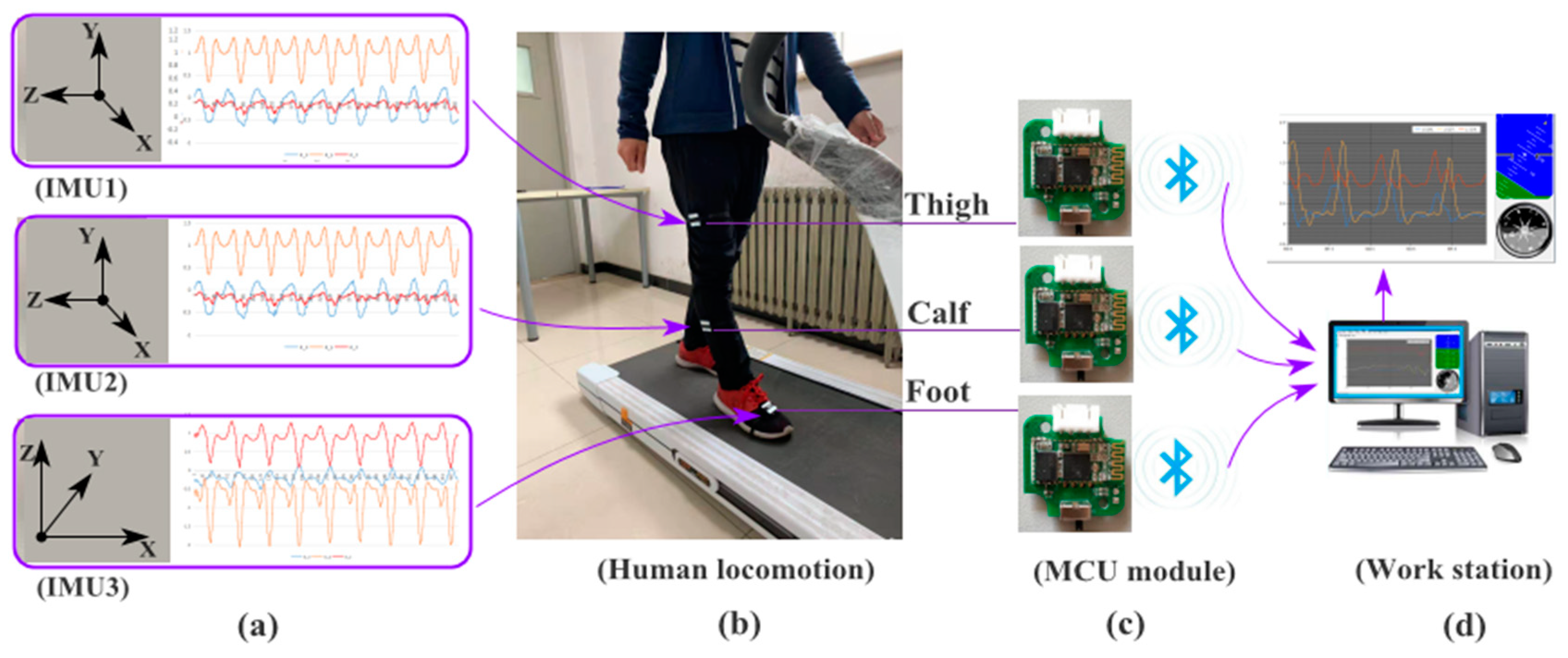
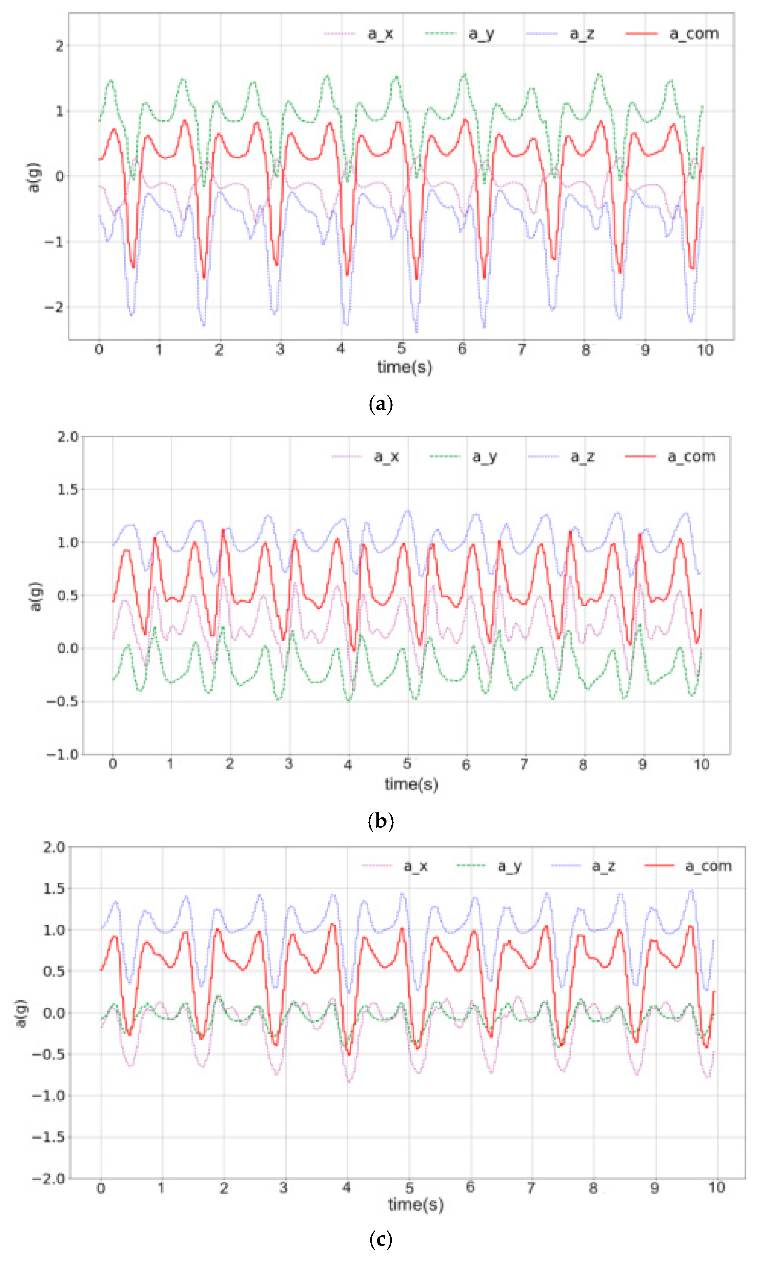
3.1. Data Collection
3.2. Data Preprocessing
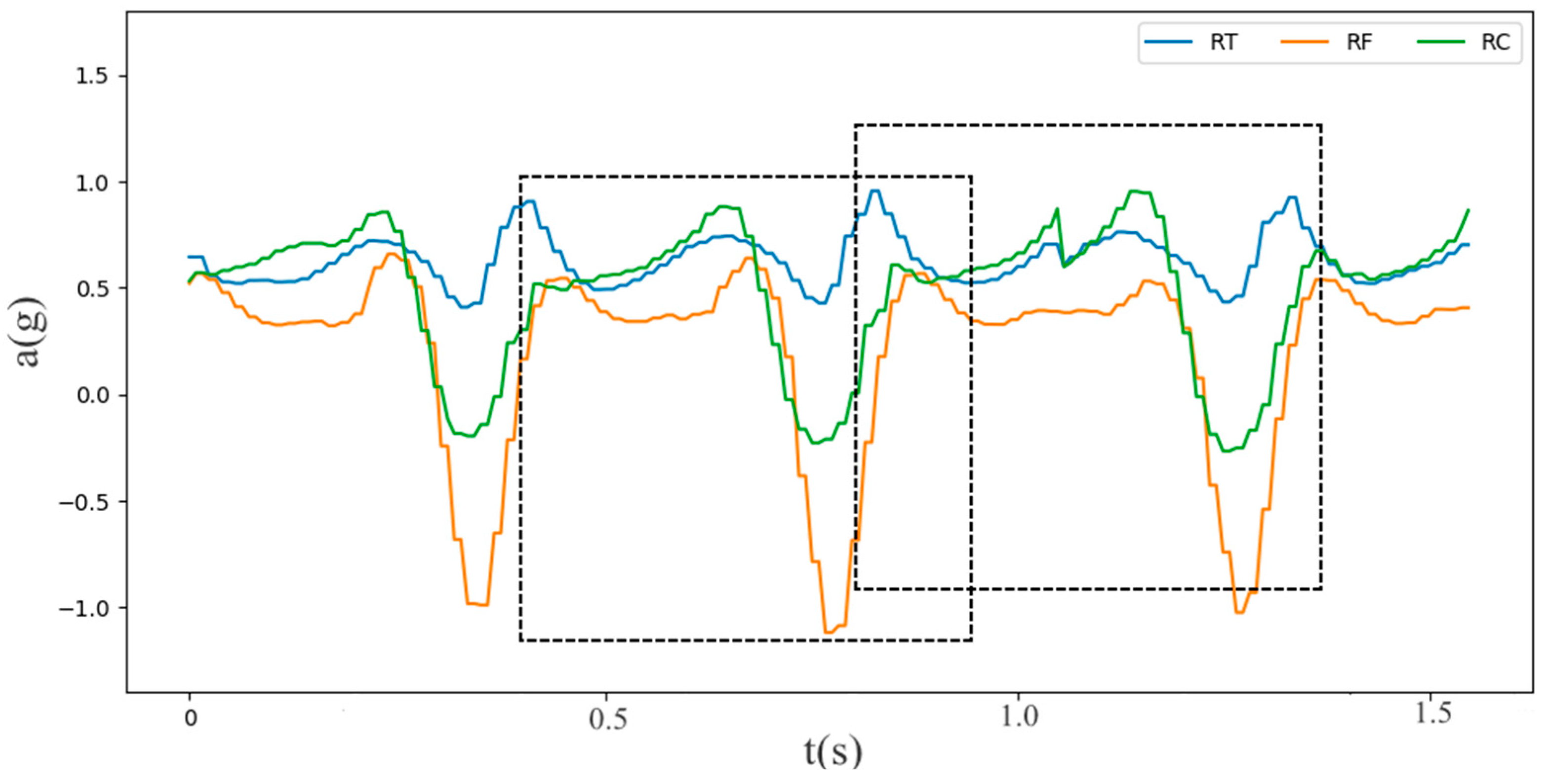
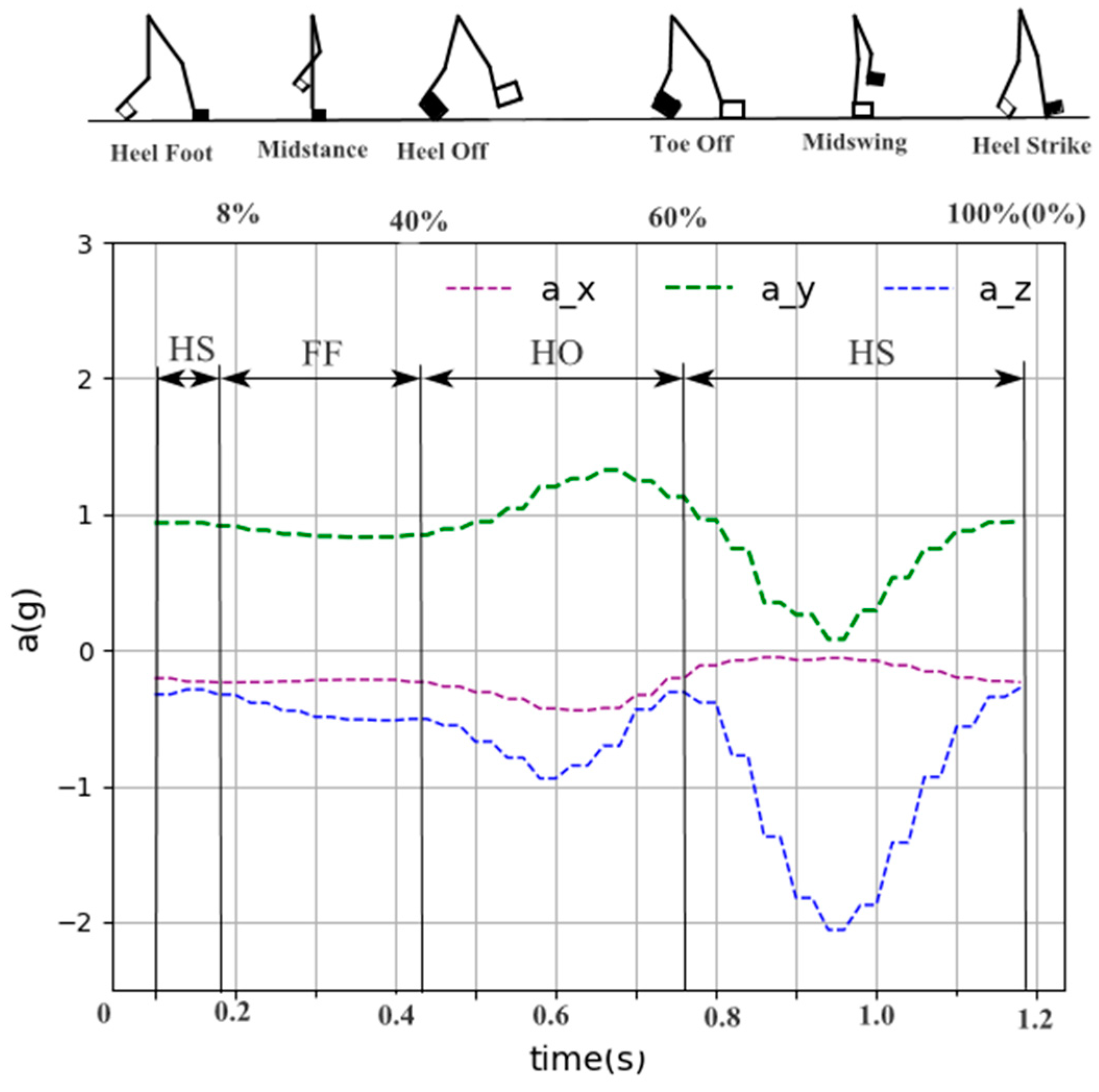
3.3. Gait Phase Division
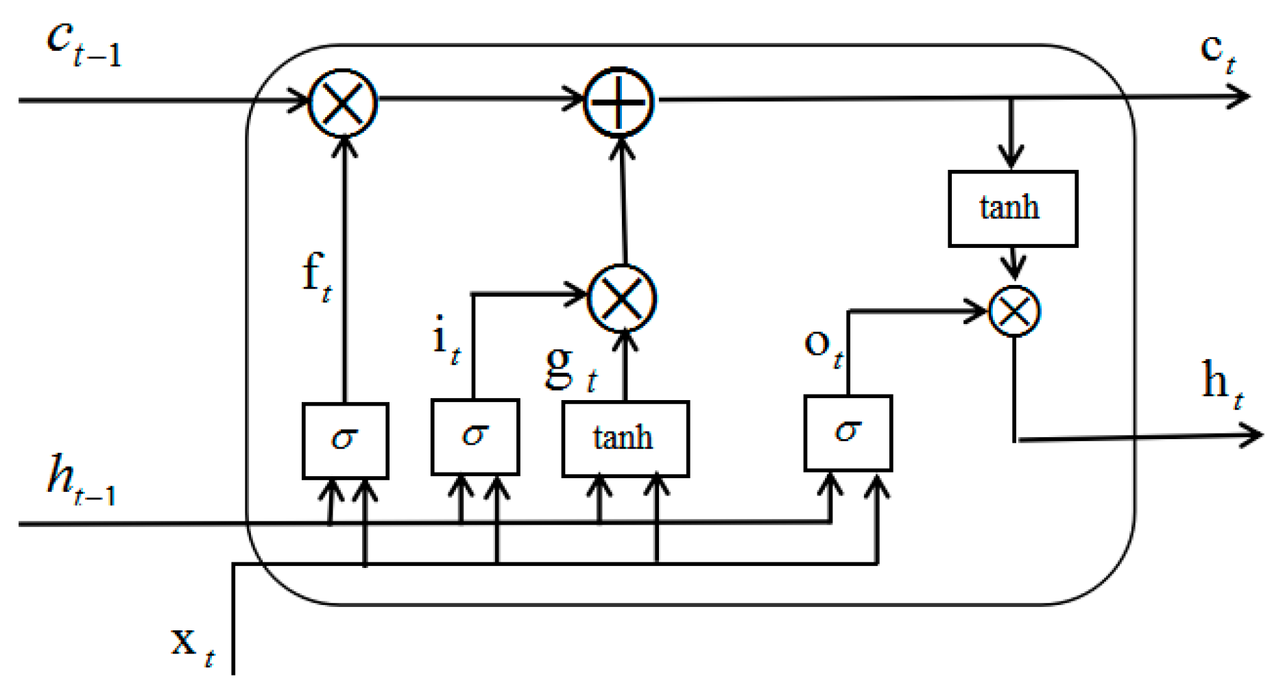
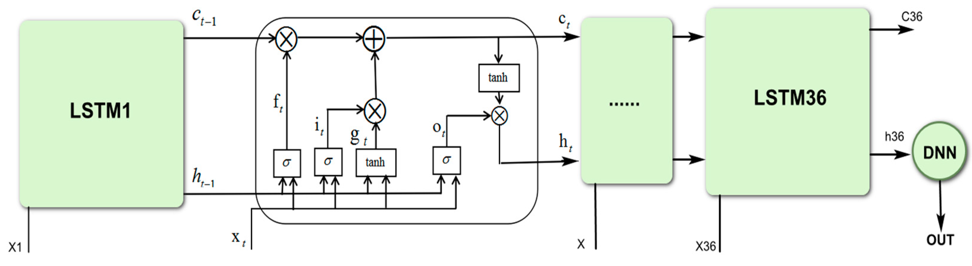
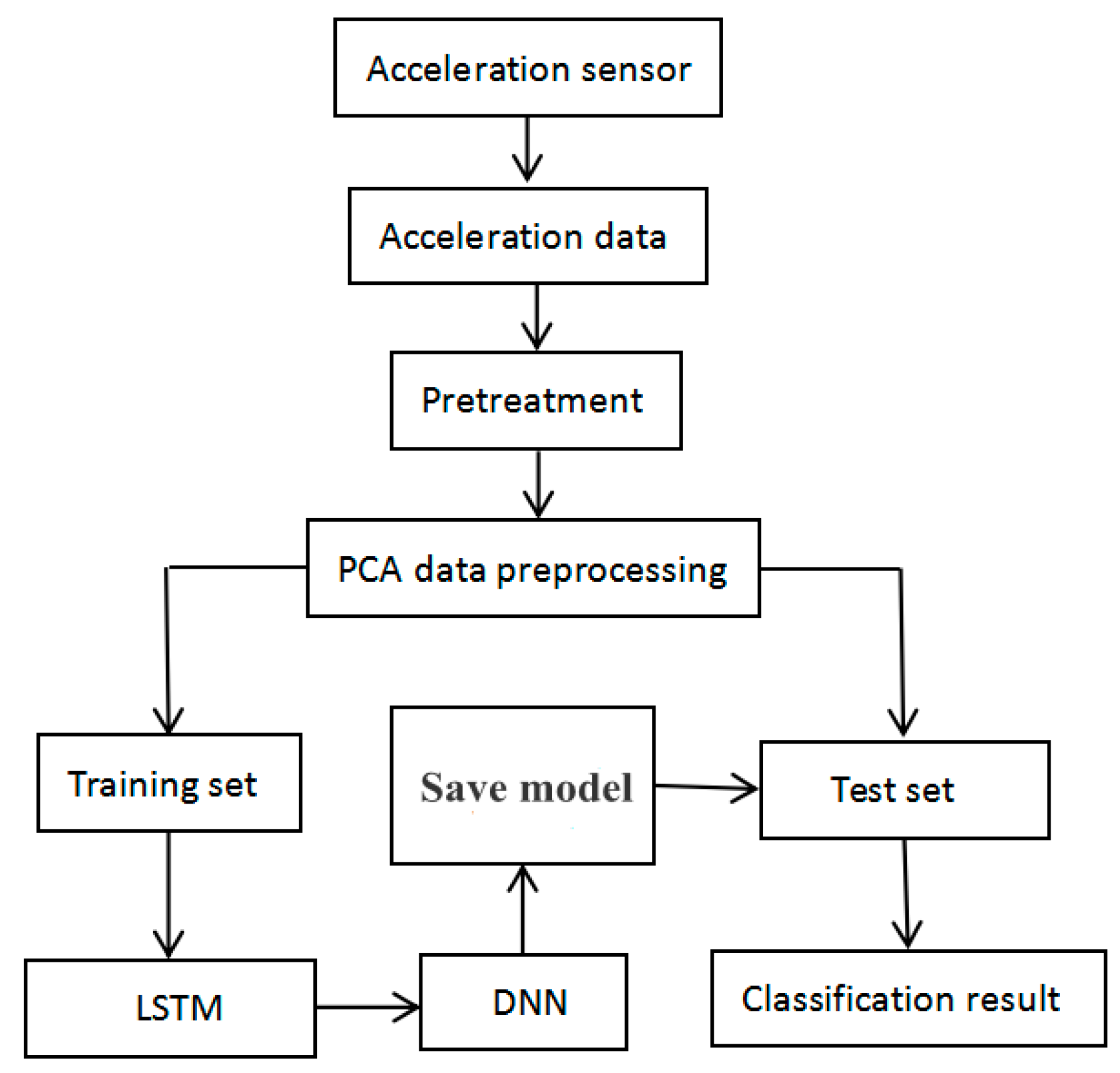
3.4. Proposed LSTM-DNN Algorithm
3.5. Evaluation Methods
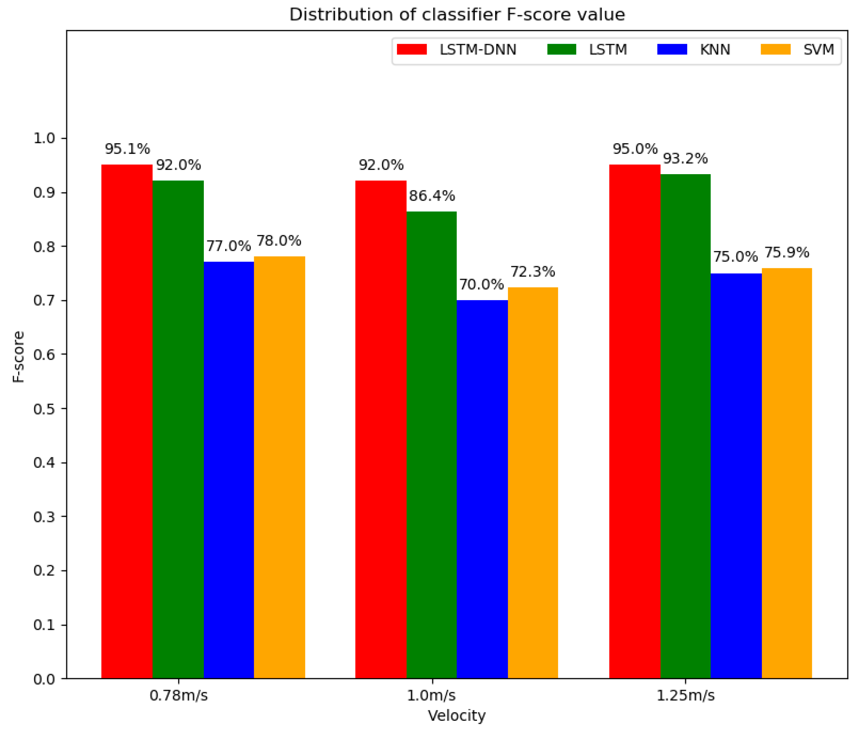
4. Experimental Results
5. Discussion
6. Conclusions
Author Contributions
Funding
Conflicts of Interest
References
- Wu, W.H.; Bui, A.A.; Batalin, M.A.; Liu, D.; Kaiser, W.J. Incremental diagnosis method for intelligent wearable sensor systems. IEEE Trans. Inf. Technol. Biomed. 2007, 11, 553–562. [Google Scholar] [CrossRef] [PubMed]
- Veneman, J.; Kruidhof, R.; Hekman, E.; Ekkelenkamp, R.; Van Asseldonk, E.; van der Kooij, H. Design and Evaluation of the LOPES Exoskeleton Robot for Interactive Gait Rehabilitation. IEEE Trans. Neural Syst. Rehabil. Eng. 2007, 15, 379–386. [Google Scholar] [CrossRef] [PubMed]
- Alexander, N.B.; Goldberg, A. Gait disorders: Search for multiple causes. Clevel. Clin. J. Med. 2005, 72, 586–594. [Google Scholar] [CrossRef] [PubMed]
- Okubo, Y.; Schoene, D.; Lord, S.R. Step training improves reaction time, gait and balance and reduces falls in older people: A systematic review and meta-analysis. Br. J. Sports Med. 2017, 51, 586–593. [Google Scholar] [CrossRef]
- Abellanas, A.; Frizera, A.; Ceres, R.; Gallego, J.A. Estimation of gait parameters by measuring upper limb-walker interaction forces. Sens. Actuators A Phys. 2010, 162, 276–283. [Google Scholar] [CrossRef]
- Figueiredo, J.; Ferreira, C.; Santos, C.P.; Moreno, J.C.; Reis, L.P. Real-Time Gait Events Detection during Walking of Biped Model and Humanoid Robot through Adaptive Thresholds. In Proceedings of the 2016 International Conference on Autonomous Robot Systems and Competitions (ICARSC), Bragança, Portugal, 4–6 May 2016; pp. 66–71. [Google Scholar]
- Vu, H.T.T.; Gomez, F.; Cherelle, P.; Lefeber, D.; Nowé, A.; Vanderborght, B. ED-FNN: A New Deep Learning Algorithm to Detect Percentage of the Gait Cycle for Powered Prostheses. Sensors 2018, 18, 2389. [Google Scholar] [CrossRef]
- Murray, S.; Goldfarb, M. Towards the use of a lower limb exoskeleton for locomotion assistance in individuals with neuromuscular locomotor deficits. In Proceedings of the 2012 Annual International Conference of the IEEE Engineering in Medicine and Biology Society, San Diego, CA, USA, 28 August–1 September 2012; Volume 2012, pp. 1912–1915. [Google Scholar]
- Yan, T.; Cempini, M.; Oddo, C.M.; Vitiello, N. Review of assistive strategies in powered lower-limb orthoses and exoskeletons. Robot. Auton. Syst. 2015, 64, 120–136. [Google Scholar] [CrossRef]
- Juri, T.; Eduardo, P.; Stefano, R.; Cappa, P. Gait Partitioning Methods: A Systematic Review. Sensors 2016, 16, 66. [Google Scholar]
- Taborri, J.; Scalona, E.; Rossi, S.; Palermo, E.; Patane, F.; Cappa, P. Real-time gait detection based on Hidden Markov Model: Is it possible to avoid training procedure? In Proceedings of the 2015 IEEE International Symposium on Medical Measurements and Applications (MeMeA), Torino, Italy, 7–9 May 2015; pp. 141–145. [Google Scholar]
- González, I.; Fontecha, J.; Hervás, R.; Bravo, J. An Ambulatory System for Gait Monitoring Based on Wireless Sensorized Insoles. Sensors 2015, 15, 16589–16613. [Google Scholar] [CrossRef]
- Anwary, A.R.; Yu, H.; Vassallo, M. Optimal foot location for placing wearable IMU sensors and automatic feature extraction for gait analysis. IEEE Sens. J. 2018, 18, 2555–2567. [Google Scholar] [CrossRef]
- Rosati, S.; Agostini, V.; Knaflitz, M.; Balestra, G. Muscle activation patterns during gait: A hierarchical clustering analysis. Biomed. Signal Process. Control 2017, 31, 1746–8094. [Google Scholar] [CrossRef]
- Goršič, M.; Kamnik, R.; Ambrožič, L.; Vitiello, N.; Lefeber, D.; Pasquini, G.; Munih, M. Online phase detection using wearable sensors for walking with a robotic prosthesis. Sensors 2014, 14, 2776–2794. [Google Scholar] [CrossRef] [PubMed]
- Yang, G.; Tan, W.; Jin, H.; Zhao, T.; Tu, L. Review wearable sensing system for gait recognition. Cluster Comput. 2018, 22, 3021–3029. [Google Scholar] [CrossRef]
- Yuwono, M.; Su, S.W.; Guo, Y.; Moulton, B.D.; Nguyen, H.T. Unsupervised nonparametric method for gait analysis using a waist-worn inertial sensor. Appl. Soft Comput. J. 2014, 14, 72–80. [Google Scholar] [CrossRef]
- Guenterberg, E.; Yang, A.Y.; Ghasemzadeh, H.; Jafari, R.; Bajcsy, R.; Sastry, S.S. A Method for Extracting Temporal Parameters Based on Hidden Markov Models in Body Sensor Networks With Inertial Sensors. IEEE Trans. Inf. Technol. Biomed. 2009, 13, 1019–1030. [Google Scholar] [CrossRef]
- Shimada, Y.; Ando, S.; Matsunaga, T.; Misawa, A.; Aizawa, T.; Shirahata, T.; Itoi, E. Clinical application of acceleration sensor to detect the swing phase of stroke gait in functional electrical stimulation. Tohoku J. Exp. Med. 2005, 207, 197. [Google Scholar] [CrossRef]
- Taborri, J.; Rossi, S.; Palermo, E.; Patanè, F.; Cappa, P. A Novel HMM Distributed Classifier for the Detection of Gait Phases by Means of a Wearable Inertial Sensor Network. Sensors 2014, 14, 16212–16234. [Google Scholar] [CrossRef]
- Kim, M.; Lee, D. Development of an IMU-based foot-ground contact detection (FGCD) algorithm. Ergonomics 2017, 60, 384–403. [Google Scholar] [CrossRef]
- Mukherjee, J.; Chattopadhyay, P.; Sural, S. Information fusion from multiple cameras for gait-based re-identification and recognition. IET Image Process. 2015, 9, 969–976. [Google Scholar]
- Ding, S.; Ouyang, X.; Li, Z.; Yang, H. Proportion-Based Fuzzy Gait Phase Detection Using the Smart Insole. Sens. Actuators A Phys. 2018, 284, 96–102. [Google Scholar] [CrossRef]
- Wang, Z.; Shibai, K.; Kiryu, T. An Internet-based cycle ergometer system by using distributed computing. In Proceedings of the 4th International IEEE EMBS Special Topic Conference on Information Technology Applications in Biomedicine, 2003, Birmingham, UK, 24–26 April 2003. [Google Scholar]
- Bejarano, N.C.; Ambrosini, E.; Pedrocchi, A.; Ferrigno, G.; Monticone, M.; Ferrante, S. A Novel Adaptive, Real-Time Algorithm to Detect Gait Events From Wearable Sensors. IEEE Trans. Neural Syst. Rehabil. Eng. 2015, 23, 413–422. [Google Scholar] [CrossRef] [PubMed]
- Caldas, R.; Mundt, M.; Potthast, W.; de Lima Neto, F.B.; Markert, B. A systematic review of gait analysis methods based on inertial sensors and adaptive algorithms. Gait Posture 2017, 57, 204–210. [Google Scholar] [CrossRef] [PubMed]
- Sánchez Manchola, M.D.; Bernal MJ, P.; Munera, M.; Cifuentes, C.A. Gait Phase Detection for Lower-Limb Exoskeletons using Foot Motion Data from a Single Inertial Measurement Unit in Hemiparetic Individuals. Sensors 2019, 19, 2988. [Google Scholar] [CrossRef] [PubMed]
- Kavanagh, J.J.; Menz, H.B. Accelerometry: A technique for quantifying movement patterns during walking. Gait Posture 2008, 28, 1–15. [Google Scholar] [CrossRef] [PubMed]
- McCamley, J.; Donati, M.; Grimpampi, E.; Mazza, C. An enhanced estimate of initial contact and final contact instants of time using lower trunk inertial sensor data. Gait Posture 2012, 36, 316–318. [Google Scholar] [CrossRef] [PubMed]
- Ma, S.Q. Research on improved pca-lda face recognition algorithm. J. Shaanxi Univ. Sci. Technol. (Nat. Sci. Ed.) 2019, 62–66. [Google Scholar]
- Parente, A.; Sutherland, J.C. PCA and Kriging for the efficient exploration of consistency regions in Uncertainty Quantification. Combust. Flame 2013, 160, 340–350. [Google Scholar] [CrossRef]
- Coussement, A.; Isaac, B.J.; Gicquel, O.; Parente, A. Assessment of different chemistry reduction methods based on principal component analysis: Comparison of the MG-PCA and score-PCA approaches. Combust. Flame 2016, 168, 83–97. [Google Scholar] [CrossRef]
- Lu, X.L.; Xu, X. Human behavior recognition based on acceleration and hga-bp neural network. Comput. Eng. 2015, 41, 220–224, 232. [Google Scholar]
- Rueterbories, J.; Spaich, E.G.; Andersen, O.K. Gait event detection for use in FES rehabilitation by radialand tangential foot accelerations. Med. Eng. Phys. 2014, 36, 502–508. [Google Scholar] [CrossRef]
- Mummolo, C.; Mangialardi, L.; Kim, J.H. Quantifying dynamic characteristics of human walking for comprehensive gait cycle. J. Biomech. Eng. 2013, 135, 91006. [Google Scholar] [CrossRef] [PubMed]
- Su, X.; Tong, H.; Ji, P. Activity recognition with smartphone sensors. J. Tsinghua Univ. (Nat. Sci. Ed.) 2014, 19, 235–249. [Google Scholar]
- Mileti, I.; Germanotta, M.; Di Sipio, E.; Imbimbo, I.; Pacilli, A.; Erra, C.; Petracca, M.; Rossi, S.; Del Prete, Z.; Bentivoglio, A.R.; et al. Measuring Gait Quality in Parkinson’s Disease through Real-Time Gait Phase Recognition. Sensors 2018, 18, 919. [Google Scholar] [CrossRef] [PubMed]
- Dong, G. Research on Human Behavior Recognition Technology Based on Multi-Feature Fusion. Master’s Thesis, Tianjin University of Technology, Tianjin, China, 2017. [Google Scholar]
- Daud, W.M.B.W.; Yahya, A.B.; Horng, C.S.; Sulaima, M.F.; Sudirman, R. Features extraction of electromyography signals in time domain on biceps brachii muscle. Int. J. Model. Optim. 2013, 3, 515–519. [Google Scholar] [CrossRef]
- Hochreiter, S.; Schmidhuber, J. Long Short-Term Memory. Neural Comput. 1997, 9, 1735–1780. [Google Scholar] [CrossRef]
- Donahue, J.; Anne Hendricks, L.; Guadarrama, S.; Rohrbach, M.; Venugopalan, S.; Saenko, K.; Darrell, T. Long-term recurrent convolutional networks for visual recognition and description. IEEE Trans. Pattern Anal. Mach. Intell. 2017, 39, 677–691. [Google Scholar] [CrossRef]
- Bai, Y.; Jin, X.; Wang, X.; Su, T.; Kong, J.; Lu, Y. Compound Autoregressive Network for Prediction of Multivariate Time Series. Complexity 2019, 2019, 9107167. [Google Scholar] [CrossRef]
- Bai, Y.T.; Wang, X.Y.; Sun, Q.; Jin, X.B.; Wang, X.K.; Su, T.L.; Kong, J.L. Spatio-Temporal Prediction for the Monitoring-Blind Area of Industrial Atmosphere Based on the Fusion Network. Int. J. Environ. Res. Public Health 2019, 16, 3788. [Google Scholar] [CrossRef] [Green Version]
- Jin, X.B.; Yang, N.; Wang, X.; Bai, Y.; Su, T.; Kong, J. Integrated predictor based on decomposition mechanism for PM2.5 long-term prediction. Appl. Sci. Basel 2019, 9, 4533. [Google Scholar] [CrossRef] [Green Version]
- Shahrebabaki, A.S.; Imran, A.S.; Olfati, N.; Svendsen, T. A Comparative Study of Deep Learning Techniques on Frame-Level Speech Data Classification. Circuits Syst. Signal Process. 2019, 38, 3501–3520. [Google Scholar] [CrossRef]
- Wang, X.; Tang, M.; Yang, S.; Yin, H.; Huang, H.; He, L. Automatic Hypernasality Detection in Cleft Palate Speech Using CNN. Circuits Syst. Signal Process. 2019, 38, 3521–3547. [Google Scholar] [CrossRef]
- Wang, C.; Li, K. Aitken-Based Stochastic Gradient Algorithm for ARX Models with Time Delay. Circuits Syst. Signal Process. 2018, 38, 2863–2876. [Google Scholar] [CrossRef]
- Zheng, Y.Y.; Kong, J.L.; Jin, X.B.; Wang, X.Y.; Su, T.L.; Wang, J.L. Probability Fusion Decision Framework of Multiple Deep Neural Networks for Fine-Grained Visual Classification. IEEE Access 2019, 7, 122740–122757. [Google Scholar] [CrossRef]
- Zheng, Y.Y.; Kong, J.L.; Jin, X.B.; Wang, X.Y.; Su, T.L.; Zuo, M. CropDeep: The Crop Vision Dataset for Deep-Learning-Based Classification and Detection in Precision Agriculture. Sensors 2019, 19, 1058. [Google Scholar] [CrossRef] [Green Version]


| Pace | Collection Location | z_1 | z_2 | z_3 |
|---|---|---|---|---|
| 0.78 m/s | Calf | 0.658 | 0.659 | 0.365 |
| Thigh | −0.556 | 0.569 | 0.365 | |
| Foot | 0.645 | 0.499 | 0.579 | |
| 1.0 m/s | Calf | 0.636 | 0.645 | 0.423 |
| Thigh | −0.479 | 0.597 | 0.643 | |
| Foot | 0.667 | 0.545 | 0.508 | |
| 1.25 m/s | Calf | 0.639 | 0.631 | 0.440 |
| Thigh | −0.565 | 0.533 | 0.630 | |
| Foot | 0.703 | 0.566 | 0.431 |
| Kernel Function | Pace | Accuracy | Precision | Recall | F-score |
|---|---|---|---|---|---|
| Linear | 0.78 m/s | 0.590 | 0.680 | 0.600 | 0.638 |
| 1.00 m/s | 0.660 | 0.710 | 0.670 | 0.689 | |
| 1.25 m/s | 0.720 | 0.720 | 0.710 | 0.715 | |
| rbf | 0.78 m/s | 0.770 | 0.780 | 0.780 | 0.780 |
| 1.00 m/s | 0.710 | 0.770 | 0.690 | 0.728 | |
| 1.25 m/s | 0.750 | 0.780 | 0.740 | 0.759 | |
| poly | 0.78 m/s | 0.490 | 0.250 | 0.500 | 0.333 |
| 1.00 m/s | 0.500 | 0.250 | 0.500 | 0.333 | |
| 1.25 m/s | 0.610 | 0.610 | 0.610 | 0.610 | |
| sigmoid | 0.78 m/s | 0.500 | 0.250 | 0.500 | 0.333 |
| 1.00 m/s | 0.610 | 0.640 | 0.600 | 0.650 | |
| 1.25 m/s | 0.630 | 0.630 | 0.630 | 0.630 |
| K | Pace | Accuracy | Precision | Recall | F-score |
|---|---|---|---|---|---|
| 2 | 0.78 m/s | 0.690 | 0.740 | 0.670 | 0.703 |
| 1.00 m/s | 0.620 | 0.700 | 0.630 | 0.663 | |
| 1.25 m/s | 0.730 | 0.760 | 0.740 | 0.750 | |
| 5 | 0.78 m/s | 0.760 | 0.780 | 0.760 | 0.770 |
| 1.00 m/s | 0.690 | 0.700 | 0.700 | 0.700 | |
| 1.25 m/s | 0.720 | 0.730 | 0.730 | 0.730 | |
| 7 | 0.78 m/s | 0.700 | 0.740 | 0.700 | 0.719 |
| 1.00 m/s | 0.680 | 0.710 | 0.680 | 0.695 | |
| 1.25 m/s | 0.640 | 0.660 | 0.630 | 0.645 | |
| 10 | 0.78 m/s | 0.670 | 0.730 | 0.660 | 0.693 |
| 1.00 m/s | 0.650 | 0.660 | 0.640 | 0.619 | |
| 1.25 m/s | 0.680 | 0.690 | 0.680 | 0.685 | |
| 15 | 0.78 m/s | 0.670 | 0.690 | 0.670 | 0.680 |
| 1.00 m/s | 0.670 | 0.680 | 0.670 | 0.675 | |
| 1.25 m/s | 0.570 | 0.690 | 0.620 | 0.653 | |
| 20 | 0.78 m/s | 0.640 | 0.680 | 0.620 | 0.649 |
| 1.00 m/s | 0.600 | 0.620 | 0.590 | 0.605 | |
| 1.25 m/s | 0.620 | 0.650 | 0.630 | 0.640 | |
| 30 | 0.78 m/s | 0.610 | 0.670 | 0.610 | 0.639 |
| 1.00 m/s | 0.620 | 0.660 | 0.630 | 0.645 | |
| 1.25 m/s | 0.520 | 0.550 | 0.510 | 0.529 |
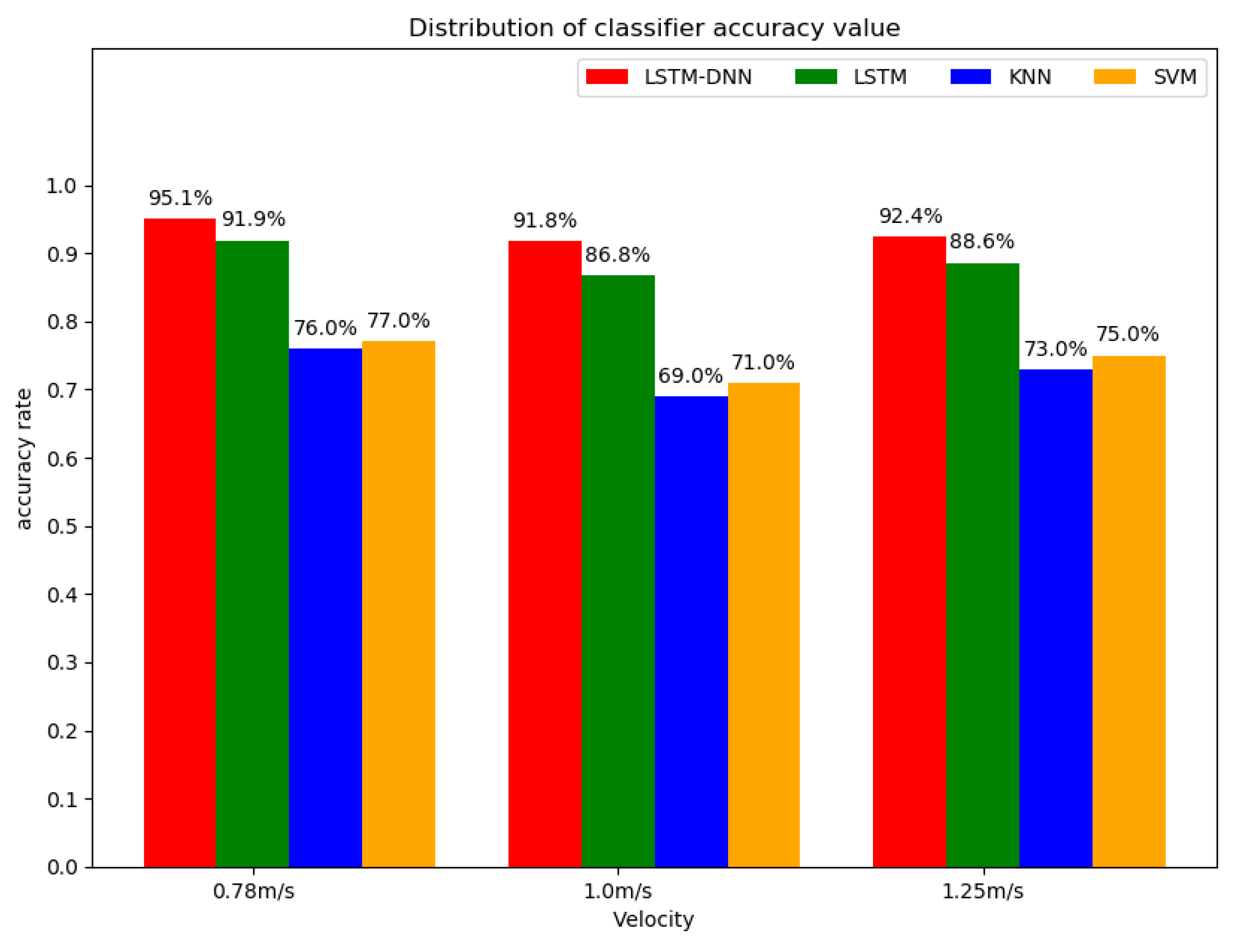
| Algorithm | Accuracy | Precision | Recall | F-score |
|---|---|---|---|---|
| LSTM-DNN | 0.951 | 0.962 | 0.941 | 0.951 |
| LSTM | 0.919 | 0.939 | 0.901 | 0.920 |
| KNN | 0.760 | 0.780 | 0.760 | 0.770 |
| SVM | 0.770 | 0.780 | 0.780 | 0.780 |
| Algorithm | Accuracy | Precision | Recall | F-score |
|---|---|---|---|---|
| LSTM-DNN | 0.918 | 0.936 | 0.905 | 0.920 |
| LSTM | 0.868 | 0.903 | 0.828 | 0.864 |
| KNN | 0.690 | 0.700 | 0.700 | 0.700 |
| SVM | 0.710 | 0.770 | 0.690 | 0.728 |
| Algorithm | Accuracy | Precision | Recall | F-score |
|---|---|---|---|---|
| LSTM-DNN | 0.924 | 0.913 | 0.946 | 0.950 |
| LSTM | 0.886 | 0.891 | 0.881 | 0.932 |
| KNN | 0.730 | 0.760 | 0.740 | 0.750 |
| SVM | 0.750 | 0.780 | 0.740 | 0.759 |
© 2019 by the authors. Licensee MDPI, Basel, Switzerland. This article is an open access article distributed under the terms and conditions of the Creative Commons Attribution (CC BY) license (http://creativecommons.org/licenses/by/4.0/).
Share and Cite
Zhen, T.; Yan, L.; Yuan, P. Walking Gait Phase Detection Based on Acceleration Signals Using LSTM-DNN Algorithm. Algorithms 2019, 12, 253. https://doi.org/10.3390/a12120253
Zhen T, Yan L, Yuan P. Walking Gait Phase Detection Based on Acceleration Signals Using LSTM-DNN Algorithm. Algorithms. 2019; 12(12):253. https://doi.org/10.3390/a12120253
Chicago/Turabian StyleZhen, Tao, Lei Yan, and Peng Yuan. 2019. "Walking Gait Phase Detection Based on Acceleration Signals Using LSTM-DNN Algorithm" Algorithms 12, no. 12: 253. https://doi.org/10.3390/a12120253
APA StyleZhen, T., Yan, L., & Yuan, P. (2019). Walking Gait Phase Detection Based on Acceleration Signals Using LSTM-DNN Algorithm. Algorithms, 12(12), 253. https://doi.org/10.3390/a12120253