A GA-SA Hybrid Planning Algorithm Combined with Improved Clustering for LEO Observation Satellite Missions

Abstract

This paper presents a space mission planning tool, which was developed for LEO (Low Earth Orbit) observation satellites. The tool is focused on a two-phase planning strategy with clustering preprocessing and mission planning, where an improved clustering algorithm is applied, and a hybrid algorithm that combines the genetic algorithm with the simulated annealing algorithm (GA–SA) is given and discussed. Experimental simulation studies demonstrate that the GA–SA algorithm with the improved clique partition algorithm based on the graph theory model exhibits higher fitness value and better optimization performance and reliability than the GA or SA algorithms alone.

1. Introduction

Earth observation satellites are important for scientific research, military reconnaissance, agricultural harvesting, and so on. With the increase of the space application scenarios, it is difficult for the in-orbit satellite resources to meet various requirements. Therefore, it is of great significance to rationally utilize limited satellite resources to obtain efficient observations. Space mission planning is a complex combinatorial optimization problem that solves the optimal satellite task planning sequence under the constraints of limited resources, time, and space.

For the satellite observation planning problem, task clustering can enable a satellite to perform more tasks with fewer sensor opening times, as shown in Figure 1 [1]. The yellow circle represents the task to be observed, and the red rectangle represents the clustering task that can perform the combined observation, where the maximum slewing ability needs to be considered. Through task clustering, several tasks can be combined at one observation activity, and the number of sensor slew times can be reduced. Meanwhile, task clustering makes it possible to accomplish some conflicting tasks at the same time [2].

Task clustering has gained more and more attention for Earth observation satellites and has been a research focus on the preprocessing field for satellite missions. Jenhn.et al. [3] proposed a branch and bound algorithm for clique partition, contributing to the development of graphic theory. In 2013, Wu G [2] proposed a two-phase scheduling method that considers task clustering of Earth observation satellites. Further, a dynamic task clustering strategy was designed by Wu G in 2017 [4]. The problem was that he did not take into account the observation duration of the task, but observed the task in the whole visible time window, which would result in the satellite resources not being used effectively. Xu Y [5] improved the classical clique partition algorithm to solve the imaging satellite task-clustering problem, but the adopted algorithm is relatively complex. Du B and Li S [6] adopted the task clustering based preprocessing method to improve the observation efficiency by combining potential targets.

It was found that in the previous investigations and studies, few constraints were considered. Hence, many research achievements are difficult to translate into practical engineering solutions. In this paper, we consider practical constraints of the sensor, including the ground resolution, time window, observation duration, maximum observation time, slewing angle, and pitching angle, and propose an improved task clustering based on the approximate clique partition algorithm proposed by Tseng [7].

Moreover, for Earth observation satellite missions, the preprocessing based on the task clustering is the first step, and the main purpose is to improve the efficiency for task planning. Compared with task clustering, research for Earth observation task planning problems are progressing rapidly. The Earth observation task planning problem is an NP (Non-deterministic Polynomial)-hard problem, and most studies use either a heuristic algorithm or an intelligent optimization algorithm to solve it. Frank et al. adopted the random search heuristic algorithm to solve the EO-1 (Earth Observing-1) system application [8]. Globus et al. [9] compared the performance of various algorithms, such as the simulated annealing algorithm, hill climbing algorithm, and genetic algorithm, for the imaging scheduling problem of point targets. Li Z proposed a multi-objective binary-encoding differential evolution (MBDE) algorithm for observation satellite proactive scheduling [10]. Kim H et al. [11] proposed the optimal scheduling algorithm for satellite formation equipped with synthetic aperture radar (SAR) imaging equipment. The proposed optimal scheduling algorithm is based on a genetic algorithm (GA). The goal is to reduce the system response time. The results show that the optimization effect of the GA algorithm is better than the particle swarm optimization (PSO) algorithm in a limited planning time. Romain studied the backtracking heuristic algorithm based on the constrained programming model [12]. Sarkheyli et al. designed a new tabu search algorithm to solve the problem when considering task priority, resource constraints, and user satisfaction in the study of mission planning for low-orbit satellites [13]. Liu S conducted mathematical modelling based on various constraints of the task planning process, and then proposed a rolling planning heuristic algorithm for the model, which divided the global task planning process into successive local planning tasks [14]. Niu X et al. designed a multi-objective genetic algorithm for fast response to natural disasters [15]. He R and Bai B established the mission planning model by considering the synthetic observation between missions; to maximize the completion of the task as the goal of optimization, a fast model annealing algorithm and a dynamic task synthesis heuristic algorithm were proposed to solve the problem [16]. Considering the priority of the task, Xu R and Chen H [17] designed a planning model and solution algorithm. Gao P et al. proposed a parallel ant colony algorithm and proved its high efficiency through experiments [18]. Jiang W solved the problem of massive user requests by designing a task merging mechanism using an adaptive ant colony algorithm [19].

Satellite task planning is a complex combination of multi-objective optimization problems. The optimization results of traditional algorithms are usually not ideal. The intelligent search algorithm is highly versatile, does not depend on specific problems, has a high search efficiency, and has an inherent parallel search capability. It is a desirable and suitable algorithm for large-scale applications. However, if a single intelligent search algorithm is used, a premature phenomenon falling into a local optimum is generally found, and the improvement of a single algorithm has some limitations. Aiming to avoid the premature phenomenon and extend the application range, a hybrid strategy combining multiple intelligent search algorithms was designed. Previous studies mostly adopted a single algorithm to solve the problem, but the optimization performance and algorithm stability were not good, and there were few constraints considered in optimization, which is quite different from the actual situation. Thus, due to the above two cases, this paper adopts a genetic algorithm–annealing algorithm (GA-SA) hybrid optimization algorithm, aiming to maximize the priority and the number of completions and considering the mission constraints including the satellite visible window, the sensor observation without overlapping, the preparation time for the sensor operation, slew angle, the observation time of the task, the single longest boot duration, the single maximum boot time, satellite energy, and data storage. A hybrid algorithm of GA and SA was developed to improve performance of satellite observation, which inherits fully the advantages of each single algorithm and the algorithms complement each other. Finally, the experimental simulation results show that the improved clustering algorithm combined with the GA-SA hybrid planning algorithm have a higher observation performance, thus improving the mission execution efficiency.

2. Review of the Improved Clustering Algorithm

The authors approached the task clustering model and algorithm early in their research using three parts: clustering constraints, the task clustering graph theory model, and the model solving algorithm [1]. The clustering preprocessing is the important part for space mission planning, which could enhance the efficiency of space missions.

Aiming to clearly demonstrate a two-phase scheduling strategy, here, a brief review of clustering preprocessing is given.

In the present paper, the practical constraints from the sensors, time window, observation duration, maximum observation time, slewing angle, and pitching angle were considered in building the clustering model. According to the constraints of the satellite clustering task, graph theory was adopted to build the clustering model. A graph $G=\langle V,E\rangle$ consists of the set of vertices $V$ and the set of edges $E$. $V({\mathrm{G}}_i)$ represents the set of tasks that can be observed in the ith orbit of the satellite. $E({\mathrm{G}}_i)$ represents the connecting line of points that meet the clustering constraint in the ith orbit. If $tas{k}_u$ and $tas{k}_v$ meet the constraint condition, then points $v_u$ and $v_v$ are connected by edge $e_{uv}$. All the edges satisfy the clustering constraints that comprise $E({\mathrm{G}}_i)$. Thus, the undirected graph model $G=\langle V,E\rangle$ can be used to represent the satellite clustering in the ith orbit among the observable original tasks.

Next, the task clustering in the graph model needs to be divided into independent cliques, as shown in Figure 2 [1]. Each independent clique represents a clustering task. In order to complete as many tasks as possible without violating the constraint conditions and improve the efficiency of satellite task completion under limited resources, the total number of clustering tasks should be as small as possible after cluster partitioning. This is a minimum clique partitioning problem, which is difficult to solve by a deterministic algorithm, but a heuristic algorithm or intelligent algorithm is generally used to solve it.

In our earlier research, the classic clique partitioning algorithm was improved, where task priority and minimum slew angle were considered as follows:

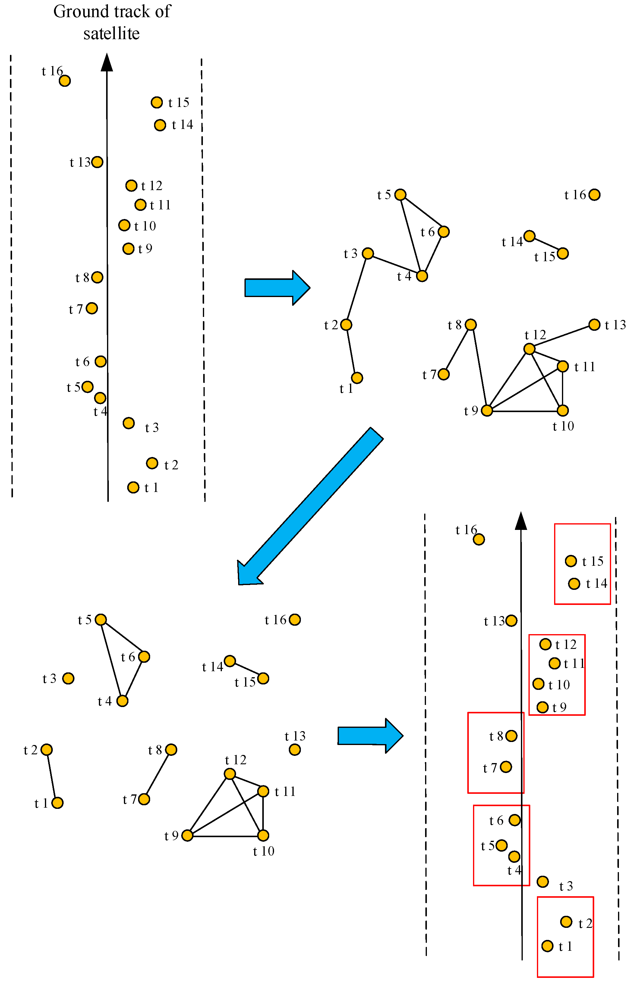
• In the cluster graph, select the edge with the largest number of common neighbors in the edge set.
• If the edge is not unique, select the edge that needs to delete the least number of edges after merging.
• If the edge is still not unique, select two vertices with higher priority and smaller clustering task slew angle to form the edge.
• Combine the two vertices of the edge into a new virtual vertex and delete the edges associated with the merged vertex to create a new edge. Update the vertex and edge collections.

Simulation results showed that the improved clique partitioning algorithm based on the graph model is an effective task clustering algorithm that can simultaneously and effectively reduce the task number size, save resources, and improve the observation efficiency [1]. Compared with the graph algorithms [2,5], the improved clique partition algorithm is relatively simple and more suitable for practical problems.

The clustering task generated by the above improved clique partitioning algorithm was taken as the input of the following task planning to carry out the optimization design.

3. Task Planning Model and Solving Algorithm

3.1. Task Planning Model

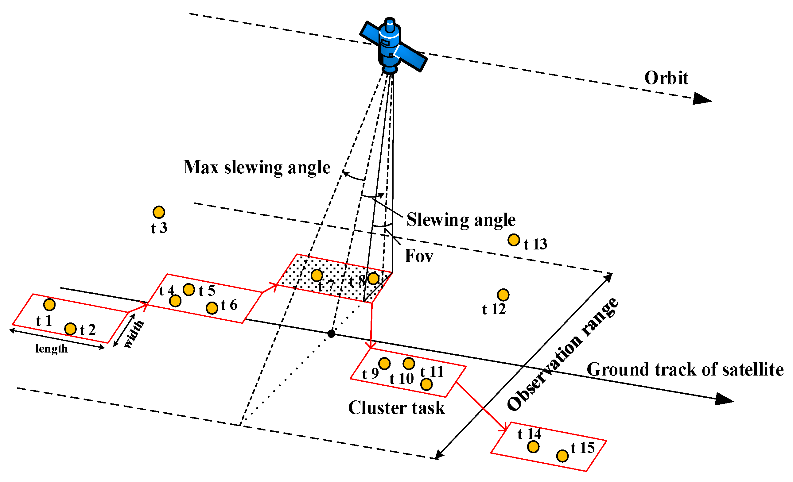
3.1.1. Main Constraints of the Planning Model

In the satellite task planning stage, the constraint satisfaction model was adopted in this paper, and the main constraint conditions are as follows:

• Observation time window constraint.

For $\forall {\complement }_{i\_u}^c\in {\complement }_i^c$,

$$\mathrm{Obser}{\mathrm{S}}_{i\_u}\ge TW{s}_{i\_u}^c, \mathrm{Obser}{E}_{i\_u}+d_u\le TW{e}_{i\_u}^c\infty .$$

(1)

In the above formula, $\mathrm{Obser}{\mathrm{S}}_i\_u$ represents the observation begin time of the clustering task ${\complement }_i^c\_u$ in the i^th orbit, $\mathrm{Obser}{E}_i\_u$ represents the observation end time, and $d_u=\mathrm{Obser}{E}_{i\_u}-\mathrm{Obser}{\mathrm{S}}_{i\_u}$ represents the observation time of task ${\complement }_i^c\_u$. $T{W}_i^c=\left\{T{W}_{i\_1}^c,T{W}_{i\_2}^c,\dots ,T{W}_{i\_N}^c\right\}$ represents a set of visible time windows for all clustering tasks ${\complement }_i^c$, $T{W}_{i\_u}^c=\left[TW{s}_{i\_u}^c,TW{e}_{i\_u}^c\right]$, where $u$ is the number of clustering tasks. The observation time window constraint ensures that the task performs observations within a visible time window.

• There can be no crossover among any two tasks, and the sensor cannot perform two tasks at the same time:

$${\displaystyle \sum _{\begin{array}{l}v=1\\ v\ne u\end{array}}^N{x}_{uv}}\le 1$$

(2)

where $x_{uv}$ represents the transition from task ${\complement }_{i\_u}^c$ to task ${\complement }_{i\_v}^c$, 1 represents the transition, and 0 represents no transition.

• There must be sufficient preparation time between any two tasks, including sensor shutdown preparation time and satellite maneuvering time:

$$\mathrm{Obser}{\mathrm{S}}_{i\_u}+d_u+s_{uv}+trans{T}_{uv}\le \mathrm{Obser}{\mathrm{S}}_{i\_v},\forall u,v\in N.$$

(3)

In the above formula, $s_{uv}$ represents the preparation time of the satellite from the end of ${\complement }_{i\_u}^c$ to the start of ${\complement }_{i\_v}^c$, $trans{T}_{uv}$ is the slew angle conversion time from task ${\complement }_{i\_u}^c$ to task ${\complement }_{i\_v}^c$, and $d_u$ is the observation time of task $TW{s}_{i\_u}^c$.

• Slew angle conversion constraint:

$$\left|\mathrm{Obser}{\mathrm{S}}_{i\_v}-\mathrm{Obser}{E}_{i\_u}\right|\ge \left|\Delta {\theta }_{i\_v}-\Delta {\theta }_{i\_u}\right|/v_s.$$

(4)

In the above formula, $\Delta {\theta }_{i\_v}$ represents the observed slew angle of task ${\complement }_i^c\_v$. $\Delta {\theta }_{i\_u}$ represents the observed slew angle of task ${\complement }_i^c\_u$. $v_s$ represents the average velocity of the satellite slew rotation. The conversion between the two tasks requires a certain amount of maneuvering time; otherwise, the observation of the two tasks cannot be completed.

• The task has certain requirements for imaging time, and the observed process needs to meet the imaging duration constraint:

$$\mathrm{Obser}{E}_i\_u-\mathrm{Obser}{\mathrm{S}}_i\_u\ge d_u.$$

(5)

Single maximum boot time constraint:

$$\max T\ge d_u(u=1,2,\dots ,N).$$

(6)

In the above formula, $\max T$ is the maximum boot time of the sensor. The observation time of the task cannot exceed the maximum start-up time of the sensor. This has been constrained in the previous task clustering section.

• Maximum boot times constraint of one orbit:

$$\mathrm{CountMax}\ge {\displaystyle \sum _{u=1}^N{x}_u}$$

(7)

where $\mathrm{CountMax}$ is the maximum number of start-up times of the sensor in one orbit and $x_u$ is the decision variable. When the satellite observes ${\complement }_{i\_u}^c$ in the current orbit, $x_u=1$; otherwise, $x_u=0$. The above equation indicates that the number of executions of all the observations within one orbit does not exceed the maximum times of the sensor.

• Energy constraint:

$${\displaystyle \sum _{u=1}^N{x}_{u}ei{d}_u}+{\displaystyle \sum _{u=1}^N{\displaystyle \sum _{\begin{array}{l}v=1\\ v\ne u\end{array}}^N{x}_{uv}(s_{uv}+trans{T}_{uv}){\epsilon }_{uv}}}\le E.$$

(8)

In the above formula, $ei$ represents the energy consumed per unit time of task completion. ${\epsilon }_{uv}$ represents the energy consumed per unit time from the end of task ${\complement }_{i\_u}^c$ to the start of task ${\complement }_{i\_v}^c$. $E$ represents the total energy available in one orbit of the satellite. $x_{uv}$ represents the transition from task ${\complement }_{i\_u}^c$ to task ${\complement }_{i\_v}^c$, 1 represents the transition, and 0 represents no transition.

• Storage capacity constraint:

$${\displaystyle \sum _{u=1}^N{\complement }_i^c\_u*ci\le M},$$

(9)

where $M$ represents the total storage capacity of the satellite in one orbit. $ci$ represents the storage capacity consumed per unit observation time.

3.1.2. Optimization Objective Function

The first optimization subobjective considers the proportion of the task priority completed by the satellite in the total task priority, which is defined as the priority function. Maximize the task priority function:

$$\max DOR=\frac{{\displaystyle \sum _{u=1}^N{x}_{u}pri{o}_u}}{{\displaystyle \sum _{u=1}^{N}pri{o}_u}}$$

(10)

where ${\complement }_i^c$ represents the set of clustering tasks within the ith orbit, ${\complement }_i^c=\{{\complement }_{i\_1}^c,{\complement }_{i\_2}^c\cdots {\complement }_{i\_N}^c\}$.$pri{o}_u$ is the priority of ${\complement }_{i\_u}^c$. $x_u$ indicates whether task ${\complement }_{i\_u}^c$ is completed. If it is completed, its value is 1; otherwise, its value is 0.

The second optimization sub-objective is to maximize the number of observation tasks.

The ratio of the number of tasks completed by the satellite to the total number of tasks is defined as the completion degree function $DOC$:

$$\max DOC=\frac{{\displaystyle \sum _{u=1}^N{x}_{u}count{\complement }_{i\_u}^c}}{count{\complement }_i^c}.$$

(11)

In the above formula, $count{\complement }_i^c$ is the number of original tasks and $count{\complement }_{i\_u}^c$ is the number of original tasks in clustering task ${\complement }_c^i$.

During the task planning process, multiple objective functions may not reach the maximum simultaneously, and the objective functions may conflict with each other. In the task planning process of this paper, we weighted two sub-objective functions and set the influence coefficients of the two subobjective functions. We considered the importance of optimizing sub-goals, and the overall goal of defining optimization is:

$$\mathrm{maxG}oal=a*\max DOR+b*\max DOC$$

(12)

where $a,b$ are the weighted influence coefficients, $a+b=1$. In this paper, the task in priority is given a greater weight. Let, $a=0.8$, and $b=0.2$.

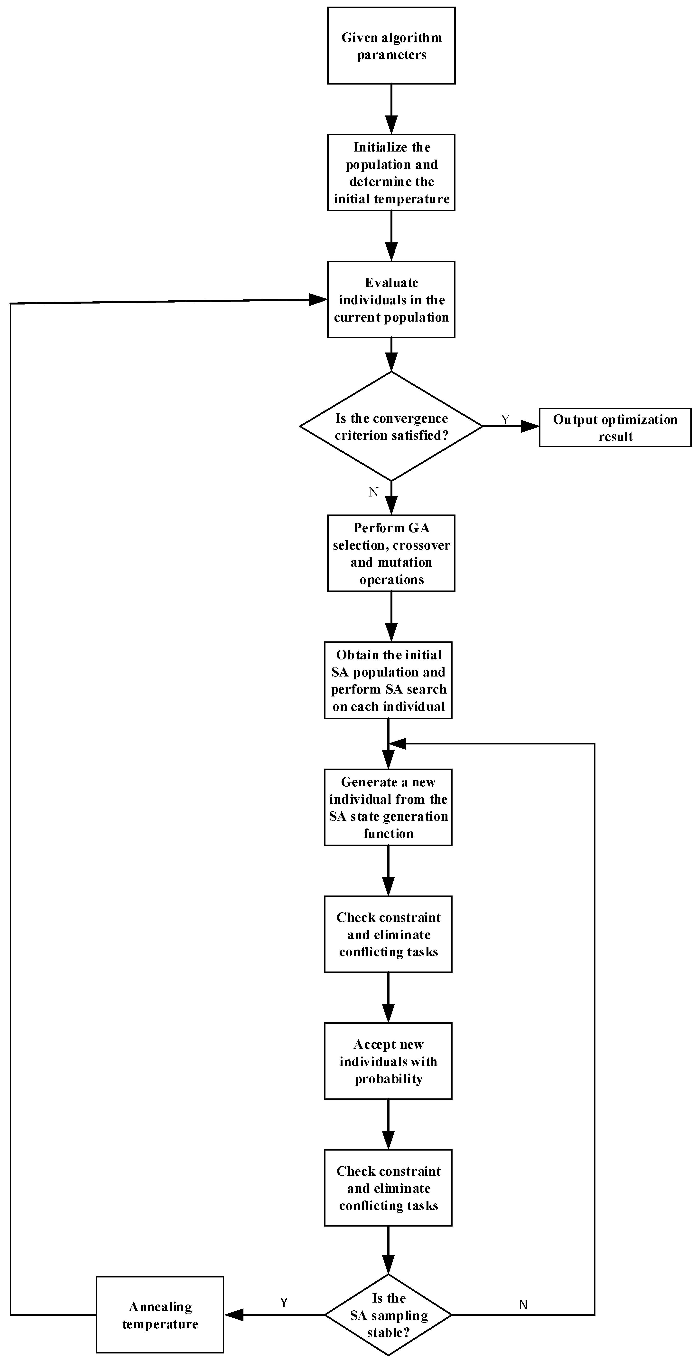
3.2. Optimization Solving Algorithm

Satellite task planning is a complex optimization problem with multiple combinations and multiple objectives. In this paper, a hybrid algorithm with the GA and SA algorithms was developed to improve the optimization performance of the algorithms, and the advantages of each single algorithm was exploited.

The combination of GA and SA improves the search ability from all aspects of the algorithm, so the choice of algorithm parameters is not necessarily very strict. When the hybrid algorithm adopts a single algorithm parameter, the optimization performance and robustness are greatly improved, especially for complex large-scale problems [20].

The GA-SA hybrid algorithm is a two-layer parallel search structure. The hybrid algorithm performs GA and SA searches sequentially at each temperature.

The initial SA solution is derived from the evolutionary GA result, and the solution obtained by SA’s metropolis sampling process becomes the initial population for further evolution in the GA. At the spatial level, the GA provides a parallel search structure to transform the SA into a parallel SA algorithm, so the hybrid algorithm always performs group parallel optimization. Figure 3 is the flow diagram of the GA-SA hybrid algorithm designed in this paper.

The following is the design process of the GA-SA hybrid algorithm:

1. GA-SA hybrid algorithm coding rules

The coding rules of the GA-SA algorithm designed in this paper adopt binary coding. The length of each individual in the population is the number of satellite clustering tasks in one orbital circle. The binary coded 1 represents the clustering task that is executed in this orbit. The 0 represents that a clustering task is not executed in this orbit (Figure 4).

2. Initial solution generation rule

In the process of generating the initial solution of the GA, an individual with all chromosome values of 1 is generated to ensure that there is an optimal fitness in the initial solution. Then, all individuals with a value of 1 are converted to corresponding decimals according to the length of the gene. The ratio of the value to the number of individuals is the coding interval between two individuals, and other individuals in the population are incremented by the value so that the initial solution of the entire GA–SA algorithm is generated. The initial solution of the SA algorithm is the individual generated by the GA after selection, crossover, and mutation.

3. GA-SA algorithm genetic operation

Crossover operation

Crossover means matching individuals in a population according to certain rules, and each pair of individuals exchanges part of their chromosomes according to a certain probability. Crossover can improve the search ability of the GA. The general steps of the crossover operation are selecting a pair of individuals to be mated from the mating pool, and then, according to the gene length L of the mating pair of individuals, randomly selecting in [1, L−1] one or more integers k as the crossover position. According to the crossover probability of the crossover operation, individuals are matched in the cross location, and genes are exchanged to form a new pair of individuals.

The crossover operation selected in this paper randomly selects two individuals from the population, calculates the fitness values of these two individuals, retains the individuals with larger fitness values, and performs the same operation again to obtain two individuals with higher fitness values; then, the crossover operation is performed on the two individuals according to the probability. Repeating this step until all individuals are selected. The probability of crossover is shown in the following formula.

$$p_c=\{\begin{array}{c}{p}_{c1}-\frac{(f_b-f_{avg})(p_{c1}-p_{c2})}{f_{\max }-f_{avg}},f_b\ge f_{avg}\\ p_{c1},f_b<f_{avg}\end{array}.$$

(13)

In the above formula, $p_{c1}=0.85,p_{c2}=0.55$, $f_b$ is the fitness value of two individuals, $f_{\max }$ is the maximum fitness value in the population, and $f_{avg}$ is the average fitness value in the population. This adaptive crossover probability can avoid early maturity and facilitate the later evolution of the algorithm [21]. When the fitness with a higher fitness value in two individuals is less than the average fitness value, the crossover probability is larger; when it is greater than the average fitness value, the crossover probability is smaller, and the range of the adaptive crossover probability is 0.55–0.85. The specific values are randomly determined within the empirical range. In this paper, we adopt a single point crossover, and the schematic diagram is shown in Figure 5.

Mutation operation

Mutation refers to the change of one or some gene values of each individual in a population to other allelic values, with a certain probability. The mutation can enhance the local search capability of the algorithm. According to the coding method, the mutation method has real value mutation and binary mutation. Binary mutation needs to negate only the corresponding gene value, and the real value mutation replaces the corresponding gene value with other random values within the range of values. The general mutation operation procedure is as follows: First, all individuals in the population are judged as to whether they will be mutated according to the pre-set mutation probability, and then, the mutated individuals are randomly selected to mutate.

In this paper, the calculation formula for individual mutation probability is similar to the crossover probability:

$$p_m=\{\begin{array}{c}{p}_{m1}-\frac{(f_c-f_{avg})(p_{m1}-p_{m2})}{f_{\max }-f_{avg}},f_c\ge f_{avg}\\ p_{m1},f_c<f_{avg}\end{array}.$$

(14)

In the above formula, $p_{m1}=0.1,p_{m2}=0.001$, $f_c$ is the fitness of the individual to be mutated, $f_{\max }$ is the maximum fitness value in the population, and $f_{avg}$ is the average fitness value in the population. When the individual fitness value is small, the mutation probability is large; when the individual fitness value is large, the mutation probability is small, and the total mutation probability range is 0.001–0.1. The specific values are randomly determined within the empirical range. The mutation method chosen in this paper is bitwise mutation, as shown in Figure 6.

Selection operation

The selection operation refers to using certain rules or methods to select some excellent individuals from the current population and pass them to the next generation according to their fitness. In this paper, the parent population and the new population generated by crossover and mutation are mixed together for selection. The specific operation is as follows: In the two generations of the population, the individual with the largest fitness is directly retained. For other individuals, two individuals are randomly selected to calculate their fitness values, the individual with the larger fitness value is retained and the operation is repeated until a new population is generated [22].

4. Fitness calculation

The fitness of each individual in the population is calculated to determine whether the individual is good or bad. In this paper, the ratio of the priority of the tasks completed by the satellite to the priority of all the tasks and the ratio of the number of tasks completed by the satellite to the number of all the tasks during the observation are taken as the optimization objective, then, the fitness value is calculated.

5. New solution to the simulated annealing algorithm

For every individual at a certain temperature, a new solution is generated by a new solution generation function, and the acceptance criteria of the new solution are based on the metropolis criterion [23]:

$$p(1\to 2)=\{\begin{array}{c}1,E_2<E_1\\ \exp (-\frac{E_2-E_1}{T}),E_2\ge E_1\end{array}$$

(15)

where $E_2$ is the energy of the newly generated solution and $E_1$ is the energy of the original solution. $E_1$ and $E_2$ are defined as the negative of the fitness value. If $E_2-E_1<0$ accept the newly generated solution, otherwise accept the newly generated solution with probability $\exp (-(E_2-E_1)/T)$. When the new solution is accepted, the current solution will be replaced with the new solution and correct the objective function value. The current individual realizes one iteration at a certain temperature and continues to the next iteration, until it reaches the number of iterations. After all the individuals in the population have finished the iteration at this temperature, the annealing process is executed and the next GA–SA algorithm iteration is carried out.

6. Checking constraints and eliminating conflicting tasks

The solution generated by the GA–SA algorithm may not necessarily satisfy the constraint conditions of satellite observation. The generated solution must be checked for constraints to determine whether these tasks conflict with each other. If any one of the constraints is not satisfied, the current solution needs to be modified to eliminate the conflicting tasks. This paper carries out two conflict checks to improve the stability of the algorithm.

7. Termination condition determination

There are two termination conditions for the GA–SA algorithm in this paper. The first one is that the simulated annealing algorithm reduces the temperature to the required temperature eps and then stops the loop iteration. The second one is that if the difference between the maximum fitness value and average fitness value in the population at a certain temperature is less than eps, then the GA–SA algorithm stops.

4. Experimental Simulation

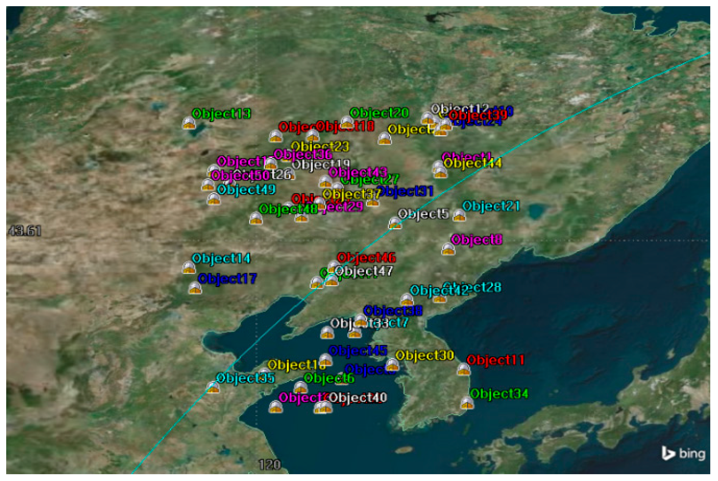
4.1. Simulation Condition

Hardware environment: Windows 10 operating system and Inter Core i7 processor. MATLAB 2016b and the System Tool Kit (STK) software were used to randomly generate 50 tasks within a certain satellite orbit. The simulation start time: 01 Apr 2018 00:00:00. The following

Table 1. Satellite orbital parameters.

a (km)	e	i	Ω	$\mathit{\omega }$	$\mathit{\upsilon }$
7000	0	60	285	0	0

and

Table 2. Satellite sensor parameters.

FOV (°)	$\mathbf{max}\mathit{T}\left(\mathbf{s}\right)$	$\mathbf{max}\mathit{\theta }\left(\text{°}\right)$
10	150	±40

show the other parameters:

These parameters are classic orbital elements. $a$ is the semimajor axis, it describes the orbit’s size. $e$ is eccentricity, it describes the orbit’s shape. $i$ is inclination, it describes the tilt of the orbital plane with respect to the fundamental plane. $\mathsf{\Omega }$ is the right ascension of the ascending node, it describes the orbital orientation with respect to the principal direction. $\omega$ is the argument of perigee, it describes the angle from the ascending node to perigee. $\upsilon$ is the true anomaly, it describes the angle from the perigee to the spacecraft’s position. The orbit parameters selected in this paper belong to the low Earth circular orbit, it is mainly for ground observation objects, and we hope to design the mission planning for some special areas in China.

If two tasks can cluster, the time window interval is $\Delta \mathrm{t}=35$.

Ground task selection: Fifty target points were randomly selected between 40 and 45° (N) latitude and 117 and 130° (E) longitude. Figure 7 is the distribution map of these 50 tasks.

The point tasks generated above are arranged in chronological order from small to large according to the starting time of the observation. The parameters of the 50 tasks are given in

Table 3. Parameters of the generated task objects.

No.	Time Window Start (s)	Time Window End (s)	Slew Angle (°)	Priority	Observation Duration	No.	Time Window Start (s)	Time Window End (s)	Slew Angle (°)	Priority	Observation Duration
1	0	0	0	2	15	26	755.31	921.78	-30.62	10	9
2	0	0	0	2	8	27	761.24	943.91	24.16	3	14
3	0	0	0	3	14	28	765.82	967.39	1.37	10	12
4	0	0	0	4	13	29	773.18	870.23	42.05	4	10
5	597.31	797.68	-0.92	1	7	30	774.55	970.67	13.88	2	13
6	616.36	799.20	-23.48	6	15	31	775.45	965.48	-19.60	8	8
7	626.61	823.31	-11.83	4	14	32	776.70	958.86	24.48	3	13
8	638.59	819.65	-24.50	3	7	33	781.49	954.96	28.35	2	12
9	645.73	801.74	-33.28	4	11	34	788.95	883.36	42.28	6	10
10	650.16	802.55	-34.14	5	8	35	789.16	933.76	36.10	8	13
11	664.20	847.74	-23.27	3	13	36	795.37	993.48	-11.44	2	10
12	668.63	832.54	-31.21	5	14	37	802.47	856.06	44.54	7	13
13	673.04	842.09	29.65	7	8	38	803.60	920.39	40.19	6	14
14	677.64	870.96	-16.21	8	11	39	810.20	934.45	39.30	0	10
15	692.36	877.29	-22.59	1	6	40	812.67	1012.95	7.53	1	10
16	692.96	844.41	34.53	8	14	41	816.26	1015.43	9.86	2	10
17	700.43	888.42	-20.69	1	8	42	827.59	1000.99	28.50	7	11
18	701.47	902.48	1.82	2	8	43	831.90	954.35	39.56	8	8
19	707.94	909.03	-1.39	5	7	44	843.73	1031.98	21.17	3	15
20	710.33	846.91	-37.25	7	6	45	844.04	980.46	37.60	4	12
21	717.58	918.66	2.14	10	8	46	844.39	918.45	43.66	7	9
22	734.11	914.19	-25.33	1	7	47	848.81	1032.19	24.10	4	13
23	742.31	902.24	32.57	2	9	48	848.82	1036.36	21.66	7	12
24	748.16	929.55	24.77	1	10	49	851.04	1029.37	26.55	1	11
25	753.34	925.03	28.94	6	10	50	853.69	1040.94	21.87	6	9

. The first four tasks are those that cannot be detected by the satellite sensor in this orbit, they are invalid tasks. The priority range of this paper is 1–10, and the observation duration is 5–15.

In the process of task planning simulation, the clustering tasks obtained by the above clustering algorithm are used as the task planning input data. The GA-SA algorithm is used for task planning, and compared with single GA and single SA algorithms. The original task numbers of 50, 100, and 150 are simulated. Some simulation parameters are as follows (

Table 4. Constraint condition parameters in the task planning process.

$\mathit{e}\mathit{i}$	${\mathit{\epsilon }}_{\mathit{u}\mathit{v}}$	$\mathit{c}\mathit{i}$	$\mathit{E}$	$\mathit{M}$	$\mathbf{CountMax}$
1	0.5	1	1200	600	60

).

In

Table 5. GA–SA algorithm parameters.

N	T0	K	${\mathit{P}}_{\mathit{S}\mathit{A}}$	eps
20	500	20	0.85	${10}^{-5}$

, N is the population size. T0 is the initial temperature. K is the number of iterations per temperature. $P_{SA}$ is the probability of new solution generation of the simulated annealing algorithm; it represents the change probability of each bit for the new state in the SA algorithm. The end condition of the algorithm is eps.

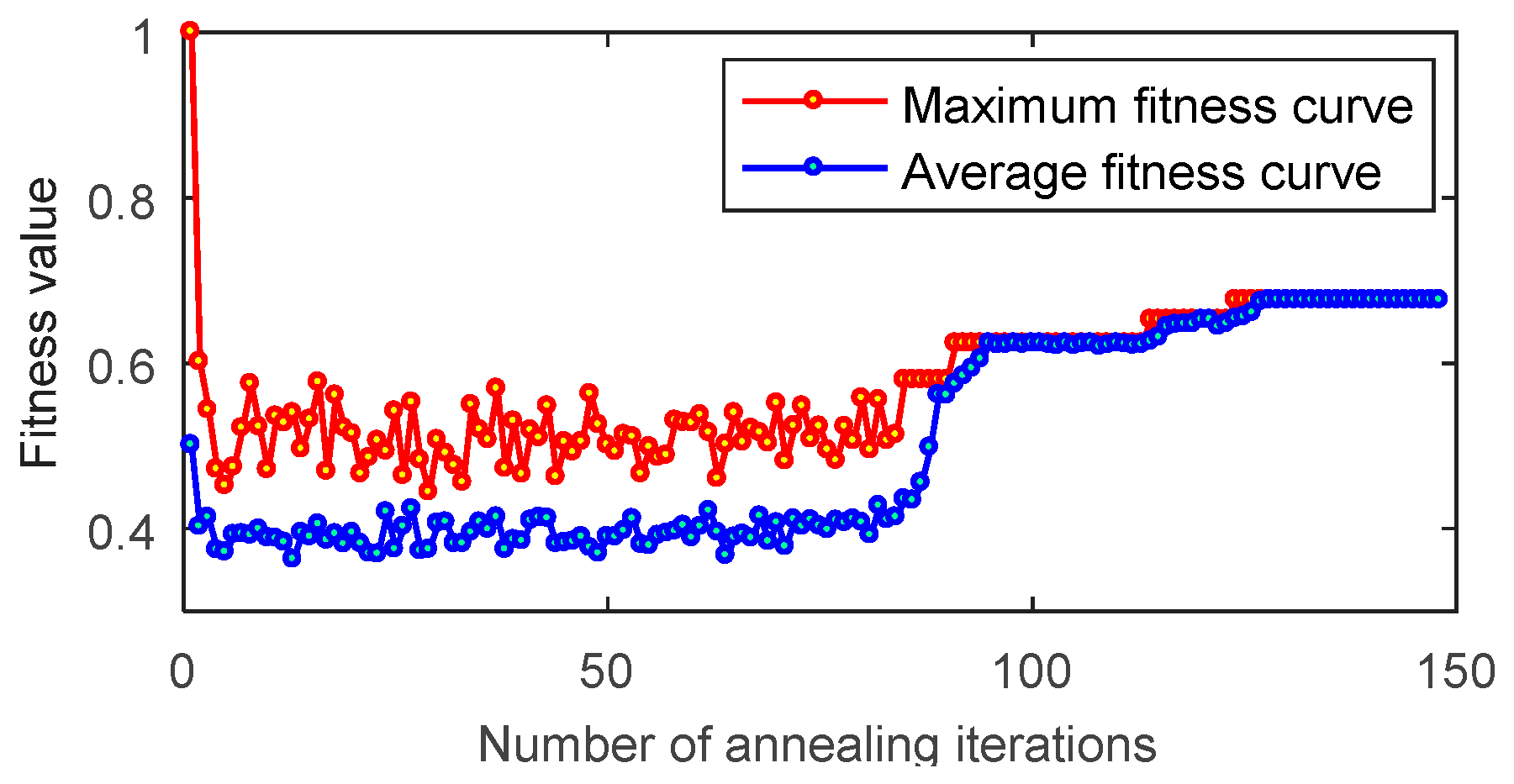
4.2. Simulation Analysis

Figure 8, Figure 9 and Figure 10 show the fitness curves of the GA-SA algorithm when the original number of tasks is 50, 100, and 150. It can be seen from the Figure that the fitness value is higher in the first iteration, because the optimal individual is retained in the initial population generation process, so the calculated fitness value is high. After checking the constraint and eliminating the conflicting tasks (the conflicting tasks are reset to zero), the fitness value is rapidly reduced. During the task planning process, the fitness value of the GA-SA is stable with the iterations increase. The final maximum fitness value and the average fitness value are basically consistent, and then reach the optimal value. It can be seen from the Figure that when the number of iterations is small, the fluctuations of the maximum fitness curve and the average fitness curve are relatively large, which is mainly caused by the randomness of the new solution of the SA algorithm when the temperature is high. As the number of iterations increases, the temperature gradually decreases, and individuals with higher fitness values are gradually retained, and the probability increases of the new SA solution being more inclined to generate individuals with higher fitness values, so the individual fitness values gradually increase and tend to be stable, and finally reach the optimal value.

When the number of tasks is different, the final optimal fitness value is different. If there are more original tasks, the final fitness value is lower. When the original number of tasks is 50, the final fitness value is 0.6294. When the original number of tasks is 100, the final fitness value is 0.3718. When the original numbers of tasks is 150, the final fitness value is 0.2833. In one orbit, the energy, storage and observation times of the satellite are limited, and satellite observations are also restricted by other constraints. Thus, satellites can execute a certain number of tasks in one orbit. As the number of satellite tasks increases, the fitness value become low.

We also compared the GA-SA algorithm with a single GA algorithm and a single SA algorithm when the number of original tasks is different. Figure 11 shows the average fitness values and variance values of the three algorithms.

Each algorithm runs ten times when the original number of tasks is 50, 100, and 150 and compares the average fitness value and variance value of the three algorithms. When the original number of tasks is 50, the average fitness value is 0.63195, and the variance value is about 3.266 × 10⁻⁷. When the original number of tasks is 100, the fitness average value is 0.3712 and variance value is approximately 1.343 × 10⁻⁷. When the original number of tasks is 150, the average fitness value is 0.28978, and the variance value is approximately 3.846 × 10⁻⁷. It can be seen from the simulation results that the GA–SA algorithm can obtain a better solution than the other two algorithms, and the average fitness value is relatively high. The variance in the GA-SA algorithm is lower than the other two algorithms, so the algorithm is more stable. This is because the GA-SA algorithm combines the advantages of the two algorithms and has parallel and serial search functions. It has stronger search ability and more sufficient search, so it can find the optimal solution within the global scope even though entering the local optimal solution is not easy. The drawback of this hybrid algorithm is longer computation times, since the GA-SA algorithm is a combination of GA and SA algorithms and the GA is especially slow. It was found that when the original number of tasks is 50, the GA algorithm runs in 1.6084 s, the SA algorithm runs in 25.4347 s, and the GA-SA algorithm runs in 171.6045 s. When the original number of tasks is 100, the GA algorithm runs in 6.6718 s, the SA algorithm runs in 33.8040 s, and the GA-SA algorithm runs in 221.0182 s. When the original number of tasks is 150, the GA algorithm runs in 9.941 s, then SA algorithm runs in 56.1382 s, and the GA-SA algorithm runs in 362.8693 s. However, for the next-generation intelligent satellite, the computation time will be determined by carrying on the high-performance OBC, which is also the main research point for our team. The combination between the GA-SA algorithm and the high-performance OBC will be studied in our future research.

5. Conclusions

In this paper, a two-phase scheduling strategy with the clustering preprocessing and mission planning were approached. In the preprocessing phase, the improved clique partitioning algorithm was applied to obtain the clustering tasks, which were the input for the task planning. In the mission planning phase, the constraint satisfaction model was established to maximize the task priority and task completion quantity, and the GA–SA hybrid algorithm was given to solve the problem. Finally, the typical experimental simulation was conducted to verify the effectiveness of the GA-SA algorithm. Simulation results show that the two-phase scheduling strategy with the task clustering preprocessing and the mission planning adopting the GA-SA hybrid algorithm can achieve the expected design goals and indicates high clustering efficiency. In addition, it was found that the GA-SA solution algorithm has higher optimization ability and reliability than the single GA or SA algorithms.

References

1. Long, X.; Wu, S.; Cui, B.; Mu, Z.; Huang, Y.; Chu, S. Analysis of satellite observation task clustering based on the improved clique partition algorithm. In Proceedings of the 2019 IEEE Congress on Evolutionary Computation (CEC), Wellington, New Zealand, 10–13 June 2019; pp. 1314–1321. [Google Scholar]
2. Wu, G.; Liu, J.; Ma, M.; Qiu, D. A two-phase scheduling method with the consideration of task clustering for earth observing satellites. Comput. Oper. Res. 2013, 40, 1884–1894. [Google Scholar] [CrossRef]
3. Jaehn, F.; Pesch, E. New bounds and constraint propagation techniques for the clique partitioning problem. Discret. Appl. Math. 2013, 161, 2025–2037. [Google Scholar] [CrossRef]
4. Wu, G.; Wang, H.; Pedrycz, W.; Li, H.; Wang, L. Satellite observation scheduling with a novel adaptive simulated annealing algorithm and a dynamic task clustering strategy. Comput. Ind. Eng. 2017, 113, 576–588. [Google Scholar] [CrossRef]
5. Xu, Y.L.; Xu, P.D.; Wang, H.L.; Peng, Y.H. Clustering of Imaging Reconnaissance Tasks Based on Clique Partition. Oper. Res. Manag. Sci. 2010, 19, 143–149. [Google Scholar]
6. Du, B.; Li, S. A new multi-satellite autonomous mission allocation and planning method. Acta Astronaut. 2018, 163, 287–298. [Google Scholar] [CrossRef]
7. Tseng, C.J.; Siewiorek, D.P. Automated synthesis of data paths in digital systems. IEEE Trans. Comput. Aided Des. Integr. Circuits Syst. 1986, 5, 379–395. [Google Scholar] [CrossRef]
8. Frank, J.; Jonsson, A.; Morris, R.; Smith, D.E.; Norvig, P. Planning and scheduling for fleets of earth observing satellites. In Proceedings of the Sixth International Symposium on Artificial Intelligence, Robotics, Automation and Space, Montreal, QC, Canada, 18–22 June 2001; p. 307. [Google Scholar]
9. Globus, A.; Crawford, J.; Lohn, J.; Pryor, A. A Comparison of Techniques for Scheduling Earth-Observing Satellites. In Proceedings of the Conference on Nineteenth National Conference on Artificial Intelligence, San Jose, CA, USA, 25–29 July 2004. [Google Scholar]
10. Li, Z.; Li, X. A multi-objective binary-encoding differential evolution algorithm for proactive scheduling of agile earth observation satellites. Adv. Space Rese. 2019, 63, 3258–3269. [Google Scholar] [CrossRef]
11. Kim, H.; Chang, Y.K. Mission scheduling optimization of SAR satellite constellation for minimizing system response time. Aerosp. Sci. Technol. 2015, 40, 17–32. [Google Scholar] [CrossRef]
12. Grasset-Bourdel, R.; Verfaillie, G.; Flipo, A. Planning and replanning for a constellation of agile Earth observation satellites. In Proceedings of the ICAPS-11 Workshop on Scheduling and Planning Applications (SPARK-11), Freiburg, Germany, 13 June 2011. [Google Scholar]
13. Sarkheyli, A.; Vaghei, B.G.; Bagheri, A. New tabu search heuristic in scheduling earth observation satellites. In Proceedings of the 2010 2nd International Conference on Software Technology and Engineering, San Juan, Puerto Rico, 3–5 October 2010; pp. 199–203. [Google Scholar]
14. Liu, S.; Chen, Y.; Xing, L.; Sun, K. Method of agile imaging satellites autonomous task planning. Comput. Integr. Manuf. Syst. 2016, 22, 928–934. [Google Scholar]
15. Niu, X.; Tang, H.; Wu, L. Satellite scheduling of large areal tasks for rapid response to natural disaster using a multi-objective genetic algorithm. Int. J. Disaster Risk Reduct. 2018, 28, 813–825. [Google Scholar] [CrossRef]
16. He, R.; Gao, P.; Bai, B.; Li, J.F.; Yao, F.; Xing, L.N. Models, algorithms and applications to the mission planning system of imaging satellites. Syst. Eng. Theory Pract. 2010, 31, 411–422. [Google Scholar]
17. Xu, R.; Chen, H.; Liang, X.; Wang, H. Priority-based constructive algorithms for scheduling agile earth observation satellites with total priority maximization. Expert Syst. Appl. 2016, 51, 195–206. [Google Scholar] [CrossRef]
18. Li, W.; Gao, P.; Chen, Y.W.; Li, J.F. A Petri Net Model and Algorithm for Remotely Sensed Data Processing Task Scheduling Problem. J. Univ. Def. Technol. 2011, 33, 138–142. [Google Scholar]
19. Jiang, W.; Pang, X. Collaborative Mission Planning for Networked Imaging Satellites; Harbin Institute of Technology Press: Harbin, China, 2016. [Google Scholar]
20. Wang, L. Intelligent Optimization Algorithms with Applications; Tsinghua University Press: Beijing, China, 2001. [Google Scholar]
21. Yu, H. The Improvement of Genetic Algorithm and It’s Application on Knapsack Problem. Master’s Thesis, Shandong Normal University, Jinan, China, 2009. [Google Scholar]
22. Yu, H.; Wang, H.; Xu, X. A genetic algorithm with competitive selection between adjacent two generations and its applications to TSP. Inf. Control 2000, 29, 309–314. [Google Scholar]
23. Bao, Z.; Yu, X. Intelligent Optimization Algorithm and Its MATLAB Example; Publishing House of Electronics Industry: Beijing, China, 2016. [Google Scholar]
Figure 1. Task clustering diagram [1].
Algorithms 12 00231 g001
Figure 2. Illustration of minimal clique partition for cluster graph [1].
Algorithms 12 00231 g002
Figure 3. The genetic algorithm–annealing algorithm (GA–SA) hybrid algorithm flow diagram.
Algorithms 12 00231 g003
Figure 4. GA-SA algorithm coding diagram.
Algorithms 12 00231 g004
Figure 5. Single-point crossover schematic.
Algorithms 12 00231 g005
Figure 6. Chromosome mutation schematic.
Algorithms 12 00231 g006
Figure 7. Task objects.
Algorithms 12 00231 g007
Figure 8. GA-SA algorithm fitness curve (50 original tasks).
Algorithms 12 00231 g008
Figure 9. GA-SA algorithm fitness curve (100 original tasks).
Algorithms 12 00231 g009
Figure 10. GA-SA algorithm fitness curve (150 original tasks).
Algorithms 12 00231 g010
Figure 11. Comparison of fitness average and variance of three algorithms.
Algorithms 12 00231 g011