Multimodal Dynamic Journey-Planning ^†

Abstract

In this paper, a new model, known as the multimodal dynamic timetable model (DTM), is presented for computing optimal multimodal journeys in schedule-based public transport systems. The new model constitutes an extension of the dynamic timetable model (DTM), which was developed originally for a different setting (unimodal journey-planning). Multimodal DTM demonstrates a very fast query algorithm that meets the requirement for real-time response to best journey queries, and an ultra-fast update algorithm for updating the timetable information in case of delays of scheduled-based vehicles. An experimental study on real-world metropolitan networks demonstrates that the query and update algorithms of Multimodal DTM compare favorably with other state-of-the-art approaches when public transport, including unrestricted—with respect to departing time—traveling (e.g., walking and electric vehicles) is considered.

1. Introduction

Mobile and web-based journey planners for scheduled public transport are plentiful, as journey-planning is a prime activity in our everyday lives. A schedule-based public transport system implies the existence of a timetable, dictating the departure and arrival times of the scheduled vehicles. This timetable is provided as input to the journey-planning problem, which asks for computing in real-time answers to the best journey queries: “Which is the best journey from a station X to another station Y, provided that a specific passenger wishes to depart at time t?”.

In its simplest setting, the journey-planning problem considers only one mode of transport (i.e., type of vehicle), and thus it is commonly referred to as the unimodal journey-planning problem. Another, more realistic setting is to consider the problem when several different transport modes (metro, bus, tram, train, car, bicycles, EVs, walking, etc.) are combined, in which case the overall problem is referred to as the multimodal journey-planning problem. In that problem, computing the best route implies employing a holistic algorithmic approach, which on the one hand takes into account each individual transport mode, and on the other hand it optimizes their choice and sequence.

The uni- or multimodal journey-planning problem specializes in a host of optimization problems, depending on the metric used and the modeling assumptions. There are two core optimization problems when one seeks to find best routes from an origin-station X to a destination-station Y: (i) The earliest arrival-time problem (EAP), where one seeks to find the best journey from X to Y that minimizes the overall travel time to reach Y; (ii) The minimum number of transfers problem (MNTP), where one seeks to find a best journey from X to Y that minimizes the total number of vehicle changes required for a passenger in order to reach Y. These two optimization criteria are often considered in combination, giving rise to multi-criteria problems. A comprehensive overview on unimodal and multimodal journey planning can be found in [1].

To meet the requirement for answering the best journey queries in real-time, the most commonly used approach for solving unimodal and multimodal journey-planning optimization problems is to carry out a preprocessing stage during which a suitable data structure is created representing the timetable information. Best journey requests are then answered by querying this data structure, and the challenge is that the structure is suitably built so that it subsequently allows for fast answering of queries. Vast literature on this approach can be found at [1] and the references therein.

Despite its simple formulation, the journey-planning problem is quite challenging, actually much more than its route-planning counterpart in road networks. The reason is that schedule-based transport possesses an inherent time-dependent component. This requires a complex modeling approach to obtain realistic results, particularly when transfer times among different vehicles should be taken into account [2].

An additional challenge in the unimodal and multimodal journey-planning setting is dealing with the delays of public transport vehicles that unfortunately occur quite often. The prime task is how to efficiently update the underlying data structure representing the timetable information so that the best journey (mostly earliest arrival (EA)) queries are still answered optimally and in real-time with respect to the new (updated after the delays) timetable.

Solving the aforementioned challenges as efficiently as possible is crucial, since otherwise the real-time response requirements posed to an actual journey planner cannot be met. An actual journey planner is usually in heavy demand—for instance, the journey planner of German railways may receive more than 420 queries per second during peak hours—and the real-time response requirements should be met both for answering queries, as well as for digesting the frequently occurred delays of schedule-based vehicles.

Our focus in this work is the multimodal journey-planning problem, for which there exist three main approaches for solving it in the literature [1]. A first approach considers a combined cost function of travel time with penalties for modal transfers (see e.g., [3,4,5]). A second approach obtains journeys that explicitly include (or exclude) certain sequences of transportation modes by building upon the label-constrained shortest path problem (see e.g., [6,7,8]. A third approach computes Pareto sets of multimodal journeys using a carefully chosen set of optimization criteria that aim at providing diverse (with respect to the transportation modes) alternative journeys (see e.g., [7,9]). Some of these approaches include flights and car driving in their modeling, both of which are beyond the scope of this paper.

In this work we investigate the multimodal schedule-based public transport problem in an urban environment that involves various transport modes (train, bus, tram) along with unrestricted ones with respect to departing time traveling. The latter includes walking and electric vehicles (EVs). The most closely related work to ours is that in [7,8], which computes multicriteria multimodal journeys.

Our prime aim is to investigate whether the recently introduced unimodal dynamic timetable model (DTM) [10], which efficiently handles EA journey-planning queries and updates the underlying timetable information structure in case of delays extremely quickly, can be extended in the multimodal setting and can provide competitive query and update times with respect to state-of-the-art approaches.

Our main contribution is Multimodal DTM (MDTM), an extension of the dynamic timetable model (DTM) [10]. MDTM can indeed model multimodal journeys, especially in urban environments, while it simultaneously offers competitive state-of-the-art query times for computing best journeys, as well as extremely fast update times for updating the timetable information in the case of delays.

We carried out a comparative experimental study on two metropolitan public transport networks (Berlin and London). Our experimental study showed that our algorithms answer multimodal EA and multicriteria queries very efficiently when public transport (train, bus, tram), along with unrestricted ones with respect to departing time traveling (walking and EVs) is considered, and remain competitive to state-of-the-art approaches even in the case of unlimited walking. In the case of delays, our timetable information structure can be updated in less than 164 microseconds on the largest input instance.

The rest of this paper is organized as follows. Section 2 presents preliminary notions and concepts regarding the modeling of timetable information and planning of (multimodal) journeys, as well as a succinct review of DTM. Section 3 presents our new mode, the multimodal DTM, along with its query and update algorithms. Section 4 presents our comparative experimental study on the two metropolitan public transport networks. Conclusions are offered in Section 5. A preliminary version of this work appeared as [11].

2. Preliminaries

The scheduled departure and arrival times of public vehicles in a (schedule-based) public transportation system is described by timetables. In this work, a timetable is a set tuple $\mathcal{T}=(\mathcal{H},\Phi ,\mathcal{C})$, where $\Phi$ is the set of stations or stops in which the passengers can get on/off a vehicle, $\mathcal{H}$ is the set of vehicles that perform the scheduled routes (e.g., train, bus, metro, or any other related means of public transport that can carry out scheduled routes), and $\mathcal{C}$ is the set of elementary connections $c=(h,S_d,S_a,t_d,t_a)$, where such an elementary connection represents the travel of a vehicle $h\in \mathcal{H}$, leaving from stop $S_d\in \Phi$ at time $t_d$ and arriving at the immediate next stop $S_a\in \Phi$ at time $t_a$. Elementary connections of schedule-based transport are restricted with respect to the scheduled departure time of the vehicles.

The realistic time-expanded model (TE-real) [2] is one of the prime models for representing a timetable. The timetable $\mathcal{T}$ in TE-real is encoded into a directed graph $G=(V,E)$ with appropriate arc weights. Every time-event (arrival or departure time of a vehicle at a station) is represented by a graph node, while the graph arcs represent either elementary connections (travel of a vehicle between consecutive stations), or transfer between different vehicles at the same station, or the waiting time between two time events (at the same station). The arc weight is the time difference between the time events associated with the endpoints of the arc.

It is worth mentioning that transfer times $\mathcal{F}$ introduce realistic transfer restrictions between vehicles. They represent the required minimum $transfer\left(S\right)$ time that a passenger needs to be transferred between different vehicles within the same stop, S.

A reduced version (TE-red) of TE-real was also presented in [2,10]. TE-red eliminates nodes representing transfer events, without losing correctness, in order to reduce the graph size.

2.1. The Dynamic Timetable Model

The dynamic timetable model (DTM) is a new model introduced in [10], aiming at efficiently updating the timetable after a vehicle delay.

Given a timetable $\mathcal{T}=(\mathcal{H},\Phi ,\mathcal{C})$, the directed graph $G=(V,E)$ representing DTM is defined as follows:

• For each stop S in $\Phi$, a switch node ${\sigma }_S$ is added to V, representing an arrival or start time event of any traveler at stop S.
• For each elementary connection $c=(h,S_d,S_a,t_d,t_a)\in \mathcal{C}$, a departure node $d_c$ (representing the time event $t_d$) is added to V, and a connection arc $(d_c,{\sigma }_{S_a})$, connecting $d_c$ to the switch node ${\sigma }_{S_a}$ of (the immediate next stop) $S_a$, is added to E.
• For each elementary connection $c=(h,S_d,S_a,t_d,t_a)\in \mathcal{C}$, a switch arc arc $({\sigma }_{S_d},d_c)$, connecting the switch node ${\sigma }_{S_d}$ of the departure stop $S_d$ to the departure node $d_c$ of c at $S_d$, is added to E.
• For each vehicle $h\in \mathcal{H}$ which travels through the itinerary $(c_1,c_2,\dots ,c_k)$, an arc (vehicle arc), connecting the departure node $d_{c_i}$ of $c_i$ with the departure node $d_{c_{i+1}}$ of $c_{i+1}$, is added to E, for each $i=1,2,\dots ,k-1$.

The timetable routes are periodic, with period $T_p$ (typically $T_p=1440=24\times 60$). Any transfer and travel time is assumed to last less than $T_p$. Given two time instances $t_1$ and $t_2$, such that $t_1\le t_2$, the (cyclic) time difference between them is denoted by $\Delta (t_1,t_2)=t_2-t_1\left(\mathrm{mod}{T}_p\right)$.

Every node and arc of G is associated with a time and weight, respectively. In particular, the associated (with nodes) time references $t:V\to {\mathbb{R}}_{\ge 0}$ and the (arc) weight function $w:E\to {\mathbb{R}}_{\ge 0}$ are defined as follows. The time-point $t\left(v\right)\in [0,T_p)$ of a departure node $v\in V$ is fixed, and it denotes the scheduled departure time of the associated public transportation vehicle. The time-point $t\left(v\right)\in [0,T_p)$ of a switch node $v\in V$ of stop $S\in \Phi$ varies and represents any possible start or arrival time at the stop S. The weight of each non-switch (i.e., connection and vehicle) arc $e=(u,v)\in E$ is fixed and set to $w\left(e\right)=\Delta \left(t\right(u),t(v\left)\right)$. The weight of the rest (i.e., switch) arcs $e\in E$ varies, and its default value is infinity.

For each connection $c=(h,S_d,S_a,t_d,t_a)$, the quantity $t_a\left(d_c\right)$ or $t_a\left(c\right)$ denotes the arrival time $t_d+w(d_c,{\sigma }_{S_a})$ at stop $S_a$, departing from $S_d$ via the departure node $d_c$, at time $t\left(d_c\right)=t_d$. For each stop, the departure nodes are ordered by their $t_a\left(d_c\right)$ values (arrival times at their arrival stop $S_a$). Moreover, for each switch node ${\sigma }_S$, we store the stop S it is associated with, while for each departure node $d_c$, we maintain both the departure time reference $t_d\left(c\right)$ and the vehicle $H\left(c\right)$ of connection c which $d_c$ is associated with.

Figure 1 shows a DTM graph. Departures of station A, labeled 20 and 35, concern train connections, while the rest concern bus connections.

2.2. Multimodal Journey

A multimodal transport network consists of schedule-based public transport along with road and pedestrian path networks, for supporting traveling with both unrestricted departure (e.g., for walking, cycling, and driving) and restricted departure (for embarking on public transport vehicles that follow scheduled timetables). In contrast to a restricted-departure timetable elementary connection, an unrestricted-departure connection $({\sigma }_{S_A},{\sigma }_{S_B})$ is defined as an arc representing a time-independent traveling path from stop $S_A$ to stop $S_B$.

A multimodal itinerary is a sequence of trip-paths consisting of unrestricted and restricted-departure connections $P=(c_1,c_2,\dots ,c_k)$ such that, for each $i=2,3,\dots ,k$, $S_a\left(c_{i-1}\right)=S_d\left(c_i\right)$ and

$$\Delta (t_a\left(c_{i-1}\right),t_d\left(c_i\right))\ge \left\{\begin{array}{cc}0\hfill & \mathrm{if}H\left(c_{i-1}\right)=H\left(c_i\right)\hfill \\ transfer\left(S_a\left(c_{i-1}\right)\right)\hfill & \mathrm{otherwise}.\hfill \end{array}\right.$$

A multimodal journey query is defined by a tuple $(S,T,t_o,M)$ where $S\in \Phi$ is a departure stop, $T\in \Phi$ is an arrival stop, $t_o$ is a minimum departure time from S, and M represents the desired transport mode(s).

There are two natural optimization criteria used to answer a timetable query. They consist in finding a multimodal itinerary from S to T starting (from S) at a time after $t_o$ and arriving at T, either with the minimum possible arrival time (Earliest Arrival—EA), or with the minimum number of vehicle transfers (Minimum Number of Transfers—MNT).

These two criteria define the following core optimization problems:

(a)

The Earliest Arrival Problem (EAP) is the problem of finding a multimodal itinerary from S to T starting at a time after $t_o$ and arriving at stop T as early as possible.

(b)

The Minimum Number of Transfers Problem (MNTP) is the problem of finding a multimodal itinerary from S to T starting at a time after $t_o$ and having as few transfers from one vehicle to another as possible.

(c)

The Multicriteria problem (MCP) that consists in finding a set of Pareto-optimal multimodal journeys from S to T starting at a time after $t_o$ with respect to the EA and MNT criteria.

(d)

The Profile problem (PRP) is the problem in which given a departure time interval I, one wishes to find all Pareto-optimal journeys from S to T with respect to EA and the latest departure time within I.

Given a timetable $\mathcal{T}$, a delay occurring on a connection c is modeled as an increase of $\delta$ minutes on the arrival time: $t_a^{\prime }\left(c\right)=t_a\left(c\right)+\delta \left(\mathrm{mod}{T}_p\right)$. The timetable is then updated according to some specific policy which depends on the network infrastructure. The new timetable, called disposition timetable ${\mathcal{T}}^{\prime }$, differs from $\mathcal{T}$ in the arrival and departure times of the vehicles that depend on $H\left(c\right)$ in $\mathcal{T}$.

In this work, we consider the simplest policy for handling delays and updating the timetable (no vehicle waits for a delayed one), which is also considered in similar works (see e.g., [10]). Other policies can be found in, for example, [12,13,14,15,16]. Therefore, when a delay occurs on a connection c, the only time references which are updated are those regarding the departure times of $H\left(c\right)$. Moreover, we assume that the policy does not take into account any possible slack times, and hence the time references are updated by adding $\delta \left(\mathrm{mod}{T}_p\right)$.

3. The Multimodal Dynamic Timetable Model

In this section, we introduce the multimodal dynamic timetable model (MDTM) aiming at modeling traveling in multimodal transport networks. We also provide the corresponding algorithms for solving EAP and MNTP, and for handling delays (updating the timetable). MDTM is an extension of DTM [10]. The key difference consists in the new ordering of the departure nodes within a stop.

Given a timetable $\mathcal{T}=(\mathcal{H},\Phi ,\mathcal{C})$, the directed graph $G=(V,E)$ representing MDTM is defined similarly to DTM (recall Section 2.1), but with the following additional features:

• For each stop $S\in \Phi$, its associated departure nodes are grouped in a specific ordering, as follows.

  (i)

  A first grouping ${\mathrm{\Gamma }}_1$ is created, where two departure nodes belong to the same group if the head switch node of their outgoing arcs is identical.

  (ii)

  A second grouping ${\mathrm{\Gamma }}_2$ is created, within each group of ${\mathrm{\Gamma }}_1$, where two departure nodes belong to the same group of ${\mathrm{\Gamma }}_2$ if the transport mode they represent is identical (i.e., departures of the same means of transport are grouped together).

  (iii)

  The departure nodes within each group of ${\mathrm{\Gamma }}_2$ are ordered by increasing arrival time at the head switch nodes of their outgoing arcs.

• For each unrestricted-departure connection from stop $S_A$ to stop $S_B$, a switch–switch arc $({\sigma }_{S_A},{\sigma }_{S_B})$ is added to G.

Let $D_{S_d}(S_a,M)$ denote a group of departure nodes resulting from the aforementioned grouping, having departure stop $S_d$, arrival stop $S_a$, and transport mode M. Figure 2 shows the MDTM graph corresponding to the DTM graph of Figure 1. Then, $D_{S_A}(S_B,bus)$ includes departure nodes 5 and 15 of stop $S_A$ that correspond to bus connections departing from $S_A$ and arriving at $S_B$.

3.1. Query Algorithm

We shall now present our query algorithm, named MDTM-QH, for solving EAP on a MDTM graph, G. An EA query $(S,T,t_s,M_{choices})$ is answered by executing a modified Dijkstra’s algorithm on G, starting from the switch node ${\sigma }_S$ of stop S.

Before discussing the details of our algorithm, we first describe the additional data structures used by MDTM-QH   with respect to the classic Dijkstra’s algorithm. In particular, for each switch node of a stop, algorithm MDTM-QH maintains a set of earliest arrival index tables, whose construction and contents are described below.

Each departure node d is associated with a departure time $t_d\left(d\right)$ and an arrival time $t_a\left(d\right)$. In general, all the departure nodes with the same departure stop $S_d$ can be ordered either by departure time or arrival time at an arrival stop. The first ordering favors an efficient search on the departure nodes to get the valid routes which have a valid departure time, i.e., a departure time greater than or equal to $t\left({\sigma }_{S_d}\right)$ at which time the traveler is at $S_d$. The second ordering favors an efficient search on the departure nodes on the optimal routes which provide the earliest arrival times to their adjacent stops. The second ordering is already applied within the existing (${\mathrm{\Gamma }}_1$ and ${\mathrm{\Gamma }}_2$) departure groups of G. However, we would also like to have the advantage of the first ordering. Therefore, for the purpose of effectively searching the departure nodes that both have valid departure times from stop $S_d$ and earliest arrival times to an adjacent arrival stop $S_a$, we introduce the earliest arrival index tables.

Let $I_{S_d}(S_a,M)$ denote an earliest arrival index table, consisting of departure nodes with departure stop $S_d$, arrival stop $S_a$, and transport mode M. $I_{S_d}(S_a,M)$ is constructed as follows: Let $d_1,d_2,\dots ,d_k\in D_{S_d}(S_a,M)$ be the sequence of the departure nodes, ordered by arrival time at $S_a$, for a trip departing from stop $S_d$ and arriving at stop $S_a$ with transport mode M. Initially, $I_{S_d}(S_a,M)$ is empty. Node $d_1$ is inserted in $I_{S_d}(S_a,M)$ and $t_{max}=t\left(d_1\right)$ is the current max departure time. Afterwards, for $i=2,\dots ,k$, if $t_{max}<t\left(d_i\right)$, then $t_{max}=t\left(d_i\right)$ and $d_i$ is inserted at the end of the $I_{S_d}(S_a,M)$ table; otherwise, $d_i$ is skipped. If the table contains the departure nodes $v_1,\dots ,v_l$, $l\le k$, and for some i, $t\left({\sigma }_{S_d}\right)\in [t\left(v_i\right),t\left(v_{i+1}\right))$, then $v_i$ is the first departure node to start the search of the earliest arrival time at $S_a$. This allows us to bypass the departure nodes, before $v_i$ in the arrival ordered sequence, with departure times less than $t\left(v_i\right)$.

Table 1. An earliest arrival index example. $I_{S_A}(S_B,M=\{bus,train\})$ includes the most important departure nodes, in terms of valid departure and earliest arrival time, with departure stop $S_A$, arrival stop $S_B$, and traveling with bus or train.

depNode	depTime	arrTime
$d_{15}$	15	20
$d_{20}$	20	37
$d_{35}$	35	46

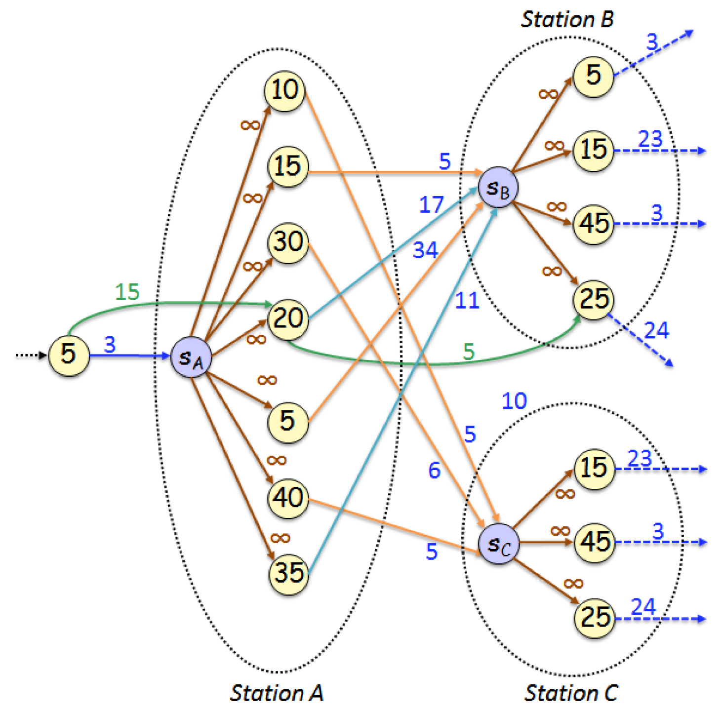
shows the contents of table $I_{S_A}(S_B,M=\{bus,train\})$, for the example shown in Figure 2. If a traveler has arrived or has started their journey from stop $S_A$ at time $t\left(s_A\right)=25>20$, then to continue at the adjacent stop $S_B$, the search of valid and optimal path-solutions can start after the departure node 20.

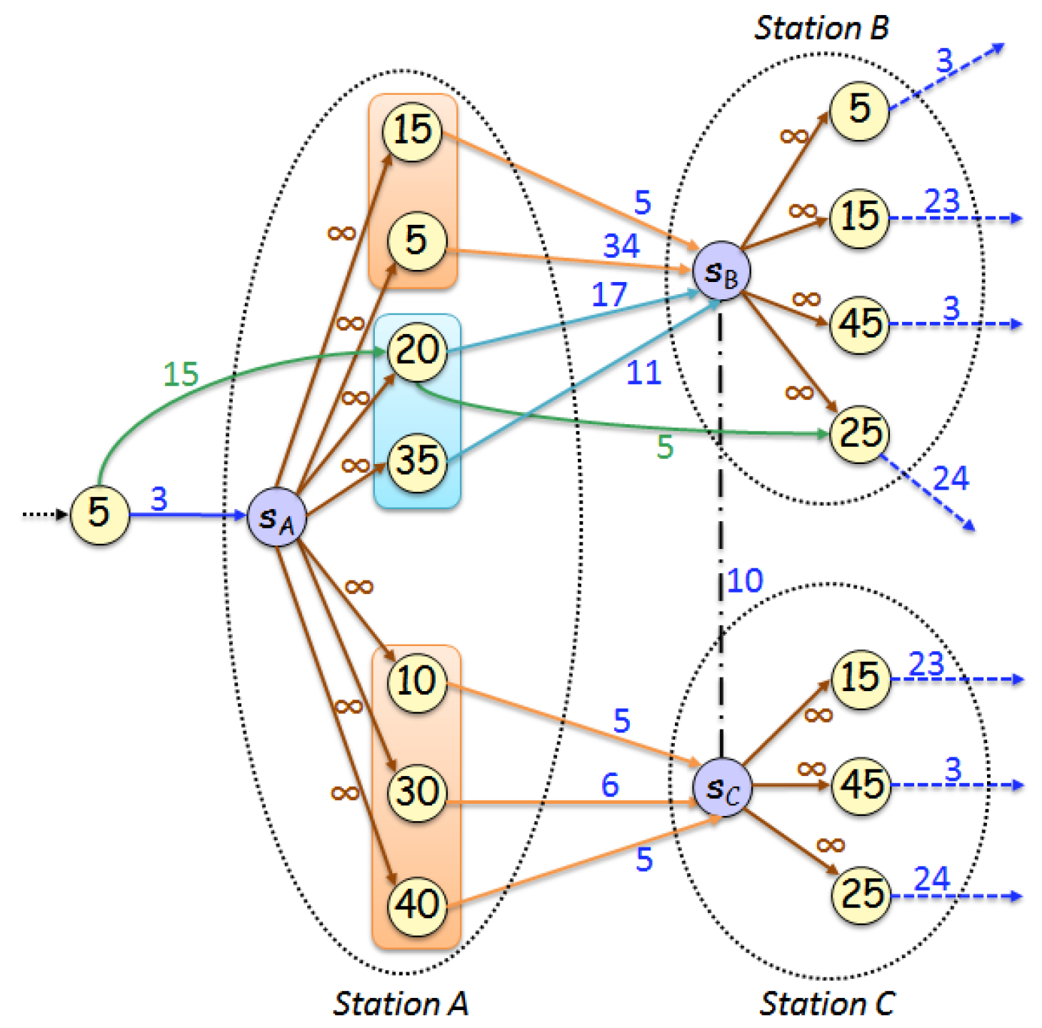
To reduce the size and the operations in the priority queue of the query algorithm, we inserted in it only the switch nodes and changed the arc relaxation as described below (iteration step). The MDTM-QH algorithm works as follows.

Initialization. The switch node ${\sigma }_{S_o}$ of the origin stop $S_o$ is inserted in the priority queue, with distance $dist\left[{\sigma }_{S_o}\right]=t_s$ and time $t\left({\sigma }_{S_o}\right)=t_s$. During the algorithm execution, provided that the traveler is already at $S_o$ at time $t_s$ the minimum transfer time of $S_o$ is set to $transfer\left(S_o\right)=0$.

Iteration. At each step, a switch node ${\sigma }_{S_x}$ is extracted from the priority queue. The node ${\sigma }_{S_x}$ is settled, having got the earliest arrival time for the optimal journey departing from $S_o$ at time $t_s$ and arriving to ${\sigma }_{S_x}$ at time $t\left({\sigma }_{S_x}\right)=dist\left[{\sigma }_{S_x}\right]\left(\mathrm{mod}{T}_p\right)$. Then, the algorithm relaxes the outgoing arcs of ${\sigma }_{S_x}$ following a node filtering and blocking process:

(i)

Using the existing grouping of departure nodes (${\mathrm{\Gamma }}_1$ and ${\mathrm{\Gamma }}_2$), the departure node groups corresponding to non-selected transportation modes are skipped.

(ii)

Using the earliest arrival index tables, the algorithm can skip the departure nodes of stop $S_x$ that have an earlier than $dist\left[{\sigma }_{S_x}\right]$ departure time, or they provide non-optimal arrival times to the next adjacent stops. In particular, after ${\sigma }_{S_x}$ is extracted, then for each adjacent arrival stop $S_a$ of stop $S_x$ and for each enabled transport mode $M\in M_{choices}$:

(1)

A binary search is performed on the index table $I_{S_x}(S_a,M)$ for getting the first departure node $d_r$ with $t\left(d_r\right)>t\left({\sigma }_{S_x}\right)$ that provides the earliest arrival time at stop $S_a$.

(2)

An arc relaxation step is performed based on those departure nodes.

Let the sequence of the outgoing switch arcs of ${\sigma }_{S_x}$ be $e_1,e_2,\dots ,e_{r-1},e_r,\dots ,e_k$, which corresponds to travel using the transport mode M and arriving at the stop $S_a$. Let $e_i=({\sigma }_{S_x},d_i)$, $i=1,\dots k$, and let the node $d_r$ be the departure node that is returned by $I_{S_x}(S_a,M)$. Within the current time period $T_p$, arcs $e_1,e_2,\dots ,e_{r-1}$ can be safely skipped, because they provide earlier departures or non-optimal arrival paths from $S_x$ to $S_a$. The first arc that is relaxed is $e_r$. Provided that the next switch arcs and their departure node heads are ordered by arrival time, the algorithm relaxes the arcs $e_r,\dots ,e_k,e_1,\dots ,e_{r-1}$ (relaxation of arcs after $e_k$ might be required, since the journey may continue on the next day) and it stops as soon as it falls over a departure node $d_i$ with (a) $\Delta (t\left({\sigma }_{S_x}\right),t\left(d_i\right))>transfer\left(S_x\right)$ and (b) $dist\left[d_i\right]+w(d_i,{\sigma }_{S_a})>dist\left[{\sigma }_{S_a}\right]+transfer\left(S_a\right)$. The first condition ensures the minimum transfer time for the traveler in using a different vehicle to continue his/her travel. The second condition ensures that we will not miss optimal paths in $S_a$ with no transfer.

In all cases, if the departure node head $d_i$ of the switch arc $e_i$ is visited for the first time, or it has a greater distance assigned during a previous step, then we set $dist\left[d_i\right]=dist\left[{\sigma }_{S_x}\right]+\Delta (t\left({\sigma }_{S_x}\right),t\left(d_i\right))$ and $w({\sigma }_{S_x},d_i)=dist\left[d_i\right]-dist\left[{\sigma }_{S_x}\right]$. When the distance is updated, the algorithm also relaxes the outgoing arcs of the departure node $d_i$. For its outgoing arc $(d_i,{\sigma }_{S_a})$, if ${\sigma }_{S_a}$ is visited for the first time or it has, from a previous step, a greater distance, then we set $dist\left[{\sigma }_{S_a}\right]=dist\left[d_i\right]+w(d_i,{\sigma }_{S_a})$. If there is also a vehicle (departure-departure) arc $(d_i,d_j)$, then for the associated vehicle we also relax the outgoing arcs of the departure nodes $d_j,\dots ,d_t$ at the next stops at which the vehicle passes along the same route. In that case, we can stop if we fall over a departure which has an outgoing arc to a switch node which has not yet been visited or extracted from the priority queue. The algorithm finishes when the switch node ${\sigma }_{S_T}$ of the destination stop $S_T$ is settled.

The MDTM-QH algorithm can be adapted to answer MNT queries by setting the weight of all switch-departure arcs to 1 (representing a transfer between vehicles) and the weight of the rest of the arcs to 0.

3.2. Improved Query Algorithm

In order to boost the performance of the query algorithm MDTM-QH, we adapted the ALT heuristic [17]. The combined algorithm is named MDTM-QH-ALT. ALT is a goal-directed technique—that is, its main aim is that of pushing the shortest-path search faster towards the target stop t. This is achieved by adding a feasible potential to the priority-key of each node in the priority queue. The feasible potentials are computed as follows. Given a set of nodes $L\subseteq V$ called landmarks, the feasible potential of a node $u\in V$ towards a target t is computed as ${\pi }_t\left(u\right)={max}_{\ell \in L}max\{dist(u,\ell )-dist(t,\ell );dist(\ell ,t)-dist(\ell ,u)\}$. By the triangle inequality, it follows that ${\pi }_t\left(u\right)$ is a lower bound to the distance $dist(u,t)$ and this is enough to prove the correctness of the shortest path algorithm (see [17] for more details). Now, the exploration and settlement of the nodes when running Dijkstra’s algorithm to compute a shortest path from a source node s to a target node t is done using the priority $dist(s,u)+{\pi }_t\left(u\right)$ for a node u, instead of $dist(s,u)$ which is used in the classical Dijkstra’s algorithm. It is easy to see that the tighter the lower bounds are, the more narrow the search space becomes—that is, the faster the query algorithm finds the shortest path. Therefore, choosing good landmarks that provide tight lower bounds is a fundamental part of the preprocessing phase of ALT.

As in [10], we apply in MDTM an approach similar to that proposed in [18]. In particular, we select as landmarks the switch nodes, each of which represents the arrival node group of a station. Therefore the lower bound distance, $dist(s_A,s_B)$, between two switch nodes, $s_A$ and $s_B$, denotes the minimum travel time among connections traveling from station A to station B. These lower bound distances can be computed during a preprocessing phase by running single-source queries from each switch node. The tightest lower bounds can be obtained by storing all pair station distances $O\left(\right|\Phi {|}^2)$ and by computing all-pairs shortest paths on the condensed version of the input graph (see [18]). This makes sense, particularly when the stations are relatively few in number.

We combined ALT along with our query algorithm in Section 3.1. This combination (MDTM-QH-ALT) considerably reduces the search space and leads to a more efficient algorithm.

3.3. The Multicriteria Multimodal Query Algorithm

In order to provide best journeys for a vector of cost functions over the multimodal transport options, we introduce the multicriteria extensions of MDTM-QH and MDTM-QH-ALT. In this case, in addition to computing journeys with a variety of transport modes, the optimal Pareto set of journeys is computed on the EA and MNT criteria (a set of pairwise non-dominating journeys, each of them being better to at least one objective criterion and no worse in all other criteria). Since it is possible that all Pareto-optimal journeys be exponential in number, we focus on finding a solution that minimizes MNT, while retaining the EA below a given threshold P (a variant also considered in [2]). Our multicriteria algorithm McMDTM-QH is described below. Its combination with ALT will be called McMDTM-QH-ALT.

Let $(S,T,t_s,M_{choices})$ be a multicriteria (EA, MNT) query, starting from the switch node ${\sigma }_S$ of stop S. The number of transfers is taken into account by setting the weight of all switch-departure arcs to 1 (representing a transfer between vehicles) and the weight of the rest of the arcs to 0. Due to the modeling, every single switch node in MDTM can have at least as many Pareto-optimal solutions as its incoming arcs. Initially, the cost minimization is on EA. Therefore, when the target switch node is settled, we have found the first (EA,MNT) Pareto optimal journey of vector distance $[R_{min},F_{max}]$, with the minimum travel time $R_{min}$, and the maximum number of transfers $F_{max}$, which is an upper bound on the number of transfers for the rest of the Pareto-optimal solutions having travel times greater than $R_{min}$. We then let Dijkstra’s algorithm continue; and whenever the target switch node is explored again with a smaller number of transfers $F_{max},F_{max}-1,F_{max}-2\dots ,0$ then a new Pareto-optimal journey is found. The algorithm stops when all journey solutions with the shortest travel time to the target stop less than or equal to $r_{mc}·R_{min}$ and transfers less than or equal to $F_{max}$, have been found.

3.4. The Profile Query Algorithm

Let $(S,T,D,M)$ be a profile query, where we need to compute all Pareto-optimal journeys from S to T, given a departure time interval $D=[dstart,dend]$, departing from S within the time interval D and arriving at T, using any chosen transport mode, including walking (with free departure) or/and public transit (with non-free departures/arrivals). The domination rule is in relation to the earliest arrival time and latest departure time. The output solution is a set of departing time subintervals and their corresponding $S\to T$ journeys that provide the minimum travel time.

Our algorithm, called PrMDTM-QH-ALT, consists of two phases.

In the first phase, the shortest path tree $R_W$ from S, using the slowest transport mode, i.e., walking, is computed. To achieve this, we run the MDTM-QH-ALT algorithm with root S and destination T, using only walking, skipping any boarding, and stopping when all switch nodes $\sigma$ with $dis{t}_W({\sigma }_S,\sigma )+{\pi }_{{\sigma }_T}\left(\sigma \right)\le dis{t}_W({\sigma }_S,{\sigma }_T)$ are explored and settled, where $dis{t}_W$ denotes the walking distance metric, and ${\pi }_{{\sigma }_T}\left(\sigma \right)\le dis{t}_W(\sigma ,{\sigma }_T)$. Let $J\in R_W\cap \Phi$ be the set of the candidate shortest path stops for the requested profile query.

In the second phase, the size of J is being considered. If J is empty, it means that there is no candidate stop for any departure time-point, and thus the shortest path by walk in the computed $R_W$ is the dominated solution in D. Otherwise, the $S\to T$ shortest journeys may include at least one of the candidate stops in J. Starting with departure time $t=dstart$, the MDTM-QH-ALT algorithm is executed, having the following preceding initialization step: the distances of the nodes $v\in R_W$ are updated with respect to the departure time t, obtaining the corresponding arrival times. Those nodes $v\in R_W$ are marked as already visited by the algorithm, and each candidate stop node in J is inserted into the priority queue.

The iteration steps of the algorithm are as follows. If the computed shortest journey from S at t towards T has at least one boarding, then a public transit itinerary has been used. Let $ar{r}_t$ be the earliest arrival time computed. In order to determine the latest departure $t_{next}=\nu +t\ge t$, $\nu \ge 0$, that the traveler can reach T at the earliest arrival time $ar{r}_t$, a backward query algorithm has to be performed [19]. Specifically, the latest departure time at S is computed by running a backward MDTM-QH-ALT algorithm, where the root is T, the incoming arcs of each settled node are traversed, and the stopping condition is the settlement of S. The computed journey $p_{ea}\left(ar{r}_t\right)$ provides a fixed minimum arrival time $a_{min}$ in $[d_{start},d_{start}+\nu ]$, with $\nu$ being the maximum waiting time in S departing at $d_{start}$ and the waiting time in S becoming zero if the departing time is at $d_{start}+\nu$. Subsequently, we continue in the remaining interval $[d_{start}+\nu +ϵ,d_{end}]$, where $ϵ>0$ denotes that the traveler cannot use the previously computed $p_{ea}\left(a_{min}\right)$ path because it is invalid—that is, at least one boarding is past, and thus the next reachable boardings in $[d_{start}+\nu +ϵ,d_{end}]$ need to be found. The next departure time-point t is set to $d_{start}+\nu +ϵ$, and the process is repeated until t reaches the last time-point, $d_{end}$. Finally, any computed journeys having travel times greater than $dis{t}_W(S,T)$ are discarded and replaced by the first-phase-computed shortest $S\to T$ path by walking.

3.5. Update Algorithm

We shall now present our update algorithm, based on [10] and named MDTM-U, for updating the timetable when a delay occurs, that is, for updating the corresponding MDTM graph.

Given a timetable $\mathcal{T}$, we assume that a delay $\delta$ occurs first on a connection $c_0$ of $\mathcal{T}$, and it is propagated to the (affected) connections $c_0,c_1,\dots ,c_k$, which are performed by the same vehicle. Also, let $d_0,d_1,\dots ,d_k$ be the departure nodes corresponding to the affected connections. If $\mathcal{T}$ is represented as a MDTM graph G, then the MDTM update algorithm computes the MDTM graph $G^{\prime }$, corresponding to the disposition timetable $\mathcal{T}$${}^{\prime }$, as follows.

• Edge weight increase: Starting with $c_0=(h,S_d,S_a,t_d,t_a)$, the weight of arc $(d_{t_d},{\sigma }_{S_a})$ is increased by $\delta$.
• Node reordering: For each of the other connections $c_i$, $i=1,\dots ,k$, its associated departure node $d_i$ has its departure time $t_d\left(d_i\right)$ increased by $\delta$. Due to that increase, the arrival time ordering of the departure nodes on the affected stops may be invalidated. Hence, along with the new arrival times, the departure node $d_i$ might need to be moved to its correct position within its group, that is, before a departure node with arrival time greater than $t_a\left(d_i\right)$.

4. Experimental Evaluation

In this section, we present our experimental study to assess the practical performance of the algorithms presented in the previous sections.

4.1. Experimental Setup

The experiments have been performed on a workstation equipped with an Intel Quad-core i5-2500K 3.30 GHz CPU and 32 GB RAM. All algorithms were implemented in C++ and compiled with gcc (v5.4.0, optimization level O3) and Ubuntu Linux (16.04 LTS).

4.2. Input Data and Parameters

The input data for creating the multimodal transport networks are (a) timetable data sets in the General Transit Feed Specification (GTFS) format, containing various means of public transport and (b) road and pedestrian network data sets in the Open Street Map (OSM) format. The integrated networks concern the metropolitan areas of Berlin and London. The source of the timetable data for London is [20] and for Berlin is [21]. The source of the road and pedestrian network data is at [22].

Table 2. Tested timetables and sizes of the corresponding graphs.

Map	$\left|\mathit{\Phi }\right|$	$\left|\mathcal{C}\right|$	TE-Real		TE-Red		DTM		MDTM
			|V|	|E|	|V|	|E|	|V|	|E|	|V|	|E|
Berlin	12,838	4,322,549	12,967,647	21,612,745	8,645,098	17,024,138	4,335,387	12,701,695	4,335,387	12,708,568
London	20,843	14,064,967	42,194,901	70,324,835	28,129,934	55,758,468	14,085,810	41,837,355	14,085,810	41,856,048

and 

Table 3. Timetable characteristics: average transfer time (mins), average degree of adjacent stops/stations, and percentage of transportation means (% of total).

$\mathcal{T}$	Berlin	London
transfer time	0.7	0.8
adjacent stops	2.7	1.2
bus	76%	98%
train	15%	2%
tram	9%

provide detailed information about the input timetables. In Table 2, we report, for each timetable, the number of stations $\left|\Phi \right|$ and the number of elementary connections $\left|\mathcal{C}\right|$ between stops (a proxy for size), as well as the number of nodes |V| and arcs |E| of the corresponding graph, for each model. In the same table we include the sizes of the realistic time-expanded (TE-real) and the reduced time-expanded models (TE-red) [2,10] for comparison. The timetable time period of the connection sets is Monday for Berlin, and Monday to Wednesday for London.

In Table 3, we report, for each timetable, the average transfer time for changing vehicles, the average number of adjacent stops or stations, and the percentage of the existing transportation means to the total number of the elementary connections.

For experimenting with MDTM, we additionally added non-restricted departure traveling paths, using the following two approaches:

• Limited walking and driving travel time paths on transitively closed pedestrian and road networks. Via the pedestrian networks, we added single foot-paths for enabling walking between nearby stops. The foot-paths that were selected and added had the shortest travel time of 10 mins at most, with walking speed being 1 m/s. Also, via the road networks, we added free-flow speed driving paths to enable driving between stops with EVs. For this scenario, we considered 10 random EV stations providing public communal EVs with the shortest travel time of 1 h at most. In addition, the driving paths connected only EV stations. In the Berlin instance, the switch–switch arcs representing foot-paths are 2381 and the driving paths are 39. In the London instance, the switch–switch arcs representing foot-paths are 412,614 and driving-paths are 60.
• Unlimited walking travel time paths on the full pedestrian network. For this purpose, we connected each switch node in the public transit network with the nearest node in the pedestrian network by an access edge. This approach was inspired by that in [19]. In the Berlin instance, the embedded pedestrian network had 932,108 nodes and 1,059,556 edges. In the London instance, the embedded pedestrian network had 1,520,056 nodes and 1,653,052 edges.

To efficiently compute the different nearest node pairs in both cases, we used the tree data structure R-tree [23] (R-tree is a balanced search tree that can order and group nearby geographical points by their minimum bounding geographical rectangle. The tree organizes its data in pages, each one of a maximum number of entries, M. The nearest neighbor search can be done efficiently in $O\left({\log }_{M}n\right)$ time, where n is the number of geographical points.)

The combination of the query algorithms with ALT requires a preprocessing phase, whose resource requirements are reported in

Table 4. MDTM ALT -based all-stop-pairs preprocessing time and space requirements for the Berlin and London instances with limited walking travel time.

$\mathcal{T}$	Berlin	London
Space (GB)	0.6	1.4
Time (mins)	0.73	1.79

and

Table 5. MDTM ALT-based preprocessing time and space requirements for the extended Berlin and London instances with unlimited walking travel time.

$\mathcal{T}$	Berlin	London
Space (GB)	0.45	0.73
Time (mins)	0.37	1.18

. In the first case, all stops are chosen as landmarks, and in the latter case, the chosen landmarks are 64 random non-departure nodes from 64 blocks in a KaHIP generated partition of the graph [24].

Contrary to the time-expanded approaches [2], the underlying MDTM graph infrastructure does not undergo any alteration during updates due to delays. For this reason, instead of using the packed-memory graph structure [25]—a robust structure supporting dynamic updates of the underlying graph— we here adopted its static version (with no empty slots), which coincides with the forward-star graph data type [26]. This provides a noticeable improvement on the memory consumption and the cache hit rate. Furthermore, as a cache-friendly priority queue, we used Sanders’ implementation of sequence heap [27] that also provides an additional improvement in query times.

Similarly to well-known observations concerning performance enhancements of Dijkstra’s algorithm [8, 33], we reordered the vertices in the graph structure so that neighboring vertices were actually located in adjacent memory blocks. This way, the cache misses are reduced and the execution times are further decreased. For this re-ordering, we used a variant of the depth first search (DFS) traversal of the graph: in each step that we visited and inserted into a LIFO queue, all the adjacent vertices from the current vertex just popped out of the queue. That is, we adopted a traversal of vertices moving as much as possible in-depth first, and followed it with a local-breadth scan.

4.3. Experimental Results

In the experimental evaluation we included the EA query algorithms TE-QH and TE-QH-ALT for TE-red [10], DTM-QH and DTM-QH-ALT for DTM [10], and the new algorithms PrMDTM-QH-ALT, MDTM-QH and MDTM-QH-ALT for MDTM. For the latter, we have also included the multicriteria (EA,MNT) query algorithms McMDTM-QH and McMDTM-QH-ALT with threshold $r_{mc}$ on EA 100% and 120% (denoted with extension 1.0 and 1.2, respectively). Note that QH denotes an optimized version of Dijkstra’s algorithm (with the corresponding node blocking and extended arc relaxation methods [10]) and QH-ALT denotes its ALT extension. For each input instance, we generated 10,000 random queries consisting of source and target stop pairs, along with a random departure time, with respect to the time period, at each source stop both for the earliest arrival queries and multicriteria queries. Also, we generated 1000 random profile queries consisting of source and target stop pairs, and a random 2 h departure time interval.

Table 6. Comparison between query algorithms. Symbol × (✓) denotes a query algorithm without (or with) ALT. McMDTM-QH-[ALT-]1.0 (McMDTM-QH-[ALT-]1.2) denotes McMDTM-QH-[ALT] with $r_{mc}=1$ ($r_{mc}=1.2$). Bullets (•) indicate the options taken into account. EA denotes an earliest arrival journey. MC denotes a multicriteria journey on arrival time and number of transfers.

Map	Algorithm			Travel Modes				Query [ms]
	ALT (×)	ALT (✓)	Object	Public Transport	Walk	EV/Car	Cycle	ALT (×)	ALT (✓)
Berlin	TE-QH [10]	TE-QH-ALT [10]	EA	•				17.50	6.28
	DTM-QH [10]	DTM-QH-ALT [10]	EA	•				27.12	11.66
	MDTM-QH	MDTM-QH-ALT	EA	•				14.24	5.71
	MDTM-QH	MDTM-QH-ALT	EA	•	•	•		15.32	8.15
London	TE-QH [10]	TE-QH-ALT [10]	EA	•				14.85	5.09
	DTM-QH [10]	DTM-QH-ALT [10]	EA	•				29.87	9.81
	MDTM-QH	MDTM-QH-ALT	EA	•				6.48	4.01
	MDTM-QH	MDTM-QH-ALT	EA	•	•	•		9.83	6.02
	McMDTM-QH-1.0	McMDTM-QH-ALT-1.0	MC	•	•	•		10.13	6.22
	McMDTM-QH-1.2	McMDTM-QH-ALT-1.2	MC	•	•	•		18.97	15.40

shows the performance of the algorithms with (✓) and without (×) the ALT heuristic for the case of limited walking (the unlimited case exhibited a similar difference in performance).

It is clear from Table 6 that the ALT-based algorithms have much better performance. For this reason, in the rest of our experimental study we considered only the ALT-based algorithms (marked with the ALT suffix).

The experimental results regarding the practical performance of the algorithms for answering multimodal queries are reported in

Table 7. Comparison between query algorithms. L-Walk (U-Walk) denotes a query algorithm with limited (unlimited) walking. McMDTM-QH-ALT-1.0 (McMDTM-QH-ALT-1.2) denotes McMDTM-QH-ALT with $r_{mc}=1$ ($r_{mc}=1.2$). Bullets (•) indicate the options taken into account. EA denotes an earliest arrival journey. MC denotes a multicriteria journey on arrival time and number of transfers (and walking duration for MCR-ht). PF denotes profiles with earliest arrival journeys with respect to the departure domain. (†) These results apply to a smaller London instance consisting of 19,746 stops and 4,695,285 elementary connections.

Map	Algorithm	Object	Travel Modes				Query [ms]
			Public Transport	Walk	EV/Car	Cycle	L-Walk	U-Walk
Berlin	TE-QH-ALT [10]	EA	•				6.28
	DTM-QH-ALT [10]	EA	•				11.66
	MDTM-QH-ALT	EA	•				5.71
	MDTM-QH-ALT	EA	•	•	•		8.15	103.46
London	TE-QH-ALT [10]	EA	•				5.09
	DTM-QH-ALT [10]	EA	•				9.81
	MDTM-QH-ALT	EA	•				4.01
	MDTM-QH-ALT	EA	•	•	•		6.02	107.93
	McMDTM-QH-ALT-1.0	MC	•	•	•		6.22	215.27
	McMDTM-QH-ALT-1.2	MC	•	•	•		15.40	360.56
	MCR-ht [7,8]	MC	•	•		•		361.23
	MR-∞-t10 [7,8]	MC	•	•		•	21.47
	PrMDTM-QH-ALT	PF(2h)	•	•			162.76	1182.12
	HLCSA [29] †	PF(2h)	•	•				1096.97
	HLRaptor [29] †	PF(2h)	•	•				733.64

. We added in Table 7 the query times of the best previous (RAPTOR-based) approaches MCR-ht and MR-∞-t10 in [7,8] (MCR-ht weakens the domination rules by trading off walking and arrival time; in MR-∞-t10 the walking duration was not used as a criterion and it was limited to 10 minutes). We stress that the former computes multicriteria (on arrival time, number of transfers, and walking duration) multimodal journeys, while the latter computes multicriteria (on arrival time and number of transfers) multimodal journeys. The times are scaled versions of those reported in [7,8] using the benchmark for scaling factors in [28].

Note that since the MCR-ht, MR-∞-t10, McMDTM-QH-ALT-1.0, and McMDTM-QH-ALT-1.2 report multicriteria multimodal queries, it is natural that they take more time than regular multimodal EA (unicriterion) query algorithms. This is also true for the case of unlimited walking, due to the much larger search space explored by the algorithms. Nevertheless, McMDTM-QH-ALT-1.0 and McMDTM-QH-ALT-1.2 are competitive to MCR-ht and MR-∞-t10.

From Table 6 and Table 7, we observe that MDTM-QH achieves a smaller query time than TE-QH and DTM-QH. This is due to the grouping and ordering of nodes within each station. In the reduced model TE-red, within each stop, the arrival time events are not merged and the departure nodes are ordered by departure time. Therefore, TE-red has a disadvantage on finding optimal paths between stops and an advantage on finding valid paths between the stops. In DTM, within each stop, the arrival time events are merged into a switch node and the departure time events are ordered by their arrival time at the next station. Therefore, DTM has an advantage of finding the optimal paths between the stops and a disadvantage of finding the valid paths between the stops. In comparison to DTM, MDTM has the departure nodes ordered by arrival time within a set of groups (${\mathrm{\Gamma }}_1$ and ${\mathrm{\Gamma }}_2$), along with the earliest arrival index tables. In that way, MDTM gains an advantage on blocking non-selected transportation modes as well as non-valid paths between the stops.

In all cases, the combination of the optimized Dijkstra’s query algorithm with the ALT goal-directed speedup technique leads to a significant decrease in query time, by at least 39%. With ALT, the query algorithms need less iterations for finding the target stop. Our multicriteria algorithms with $r_{mc}=1.0$ are faster than those with $r_{mc}=1.2$, since they compute less journeys.

In the case of profile queries with a departure time interval of 2 h, the computation cost is higher. Such queries involve the execution of several earliest arrival queries on different departure times, considering any optimal reachable boarding via public transport that provides the minimum travel time at the chosen destination. Algorithms HLCSA [29] and HLRaptor [29] are extensions of CSA [30] and Raptor [31], respectively, requiring substantial prepossessing time for producing the hub labels. In particular, the hub labeling walking graph data of both algorithms are obtained from [32] and their computation on a dual 10-core Intel Xeon E5-2670-v2 CPU [29] (a server much more powerful than ours) requires about 4 h. Both HLCSA and HLRaptor are designed to efficiently compute journeys with unrestricted walking. Comparing HLCSA, HLRaptor, and PrMDTM-QH-ALT, we see a trade-off, but we need to stress that the implementations were applied on different London instances. The hub labeling algorithms provide (by design) faster query times at the expense of heavy preprocessing, but they were applied on a much smaller London instance (consisting of 19,746 stops and 4,695,285 elementary connections). PrMDTM-QH-ALT has an extremely fast preprocessing time at the expense of a (not so much) slower query time, but it was applied on an instance three times larger (consisting of 20,843 stops and 14,064,967 elementary connections) than that used by HLCSA and HLRaptor. The implementations of HLCSA and HLRaptor tested in our experimental study were taken from [33]. The average number of journeys which need to be computed in the profile solution set is about 14.

For evaluating updates (occurring after a delay), 10,000 elementary connections were randomly selected for each input instance, and for each elementary connection we randomly generated a delay affecting the corresponding train or bus, chosen with uniform probability distribution between 1 and 360 min.

In the experimental evaluation we have included the update algorithms TE-UH for TE-red [10], DTM-U for DTM [10], and the new algorithm MDTM-U for MDTM. The experimental results of the update algorithms are reported in

Table 8. Comparison among update algorithms for the TE-red, DTM, and MDTM models.

Instance	Algorithm	Travel Modes		Update [$\mathsf{\mu }$s]
		Bus	Train
Berlin	TE-UH [10]	•	•	249.3
	DTM-U [10]	•	•	85.7
	MDTM-U	•	•	87.2
London	TE-UH [10]	•	•	484.6
	DTM-U [10]	•	•	148.1
	MDTM-U	•	•	163.1

. The update times measure the average computational times for updating the graph when a delay in a transportation vehicle itinerary has to be absorbed. In DTM-U, only (at most) two arc weights and a few node time references need to be changed in the original graph to keep the EA queries correct. Although MDTM-U has an additional computation cost to maintain the earliest arrival index table for any node time reference update, the time of MDTM-U is competitive to that of the DTM-U. The updating algorithm in both cases takes less than 164 $\mathsf{\mu }$s. That is due to the fact that the number of stations where something changes, as a consequence of a delay, is small with respect to the size of the whole set of stations $\left|\Phi \right|$.

5. Conclusions and Future Work

In this work, a new model for multimodal route planning in schedule-based public transport systems, called Multimodal DTM, was presented that constitutes an extension of the dynamic timetable model (DTM), originally developed for unimodal journey-planning in [10]. An extensive experimental study showed that Multimodal DTM compares favorably with other state-of-the-art multimodal route planners.

We are currently developing a mobile application for multimodal route planning, using Multimodal DTM as the core routing engine of the cloud-residing component. Our multimodal journey planner can also be combined with the mobile application developed in [34] that allows users to evaluate the routes suggested (by the planner). We are also working on developing multicriteria multimodal journeys with more (than two) traveling options/criteria.

References

1. Bast, H.; Delling, D.; Goldberg, A.V.; Müller-Hannemann, M.; Pajor, T.; Sanders, P.; Wagner, D.; Werneck, R.F. Route planning in transportation networks. In Algorithm Engineering—Selected Results and Surveys; Lecture Notes in Computer Science; Springer: Cham, Switzerland, 2016; Volume 9220, pp. 19–80. [Google Scholar]
2. Pyrga, E.; Schulz, F.; Wagner, D.; Zaroliagis, C. Efficient models for timetable information in public transportation systems. ACM J. Exp. Algorithm. 2008, 12, 2–4. [Google Scholar] [CrossRef]
3. Aifadopoulou, G.; Ziliaskopoulos, A.; Chrisohoou, E. Multiobjective optimum path algorithm for passenger pretrip planning in multimodal transportation networks. J. Transp. Res. Board 2007, 2032, 26–34. [Google Scholar] [CrossRef]
4. Antsfeld, L.; Walsh, T. Finding multi-criteria optimal paths in multi-modal public transportation networks using the transit algorithm. In Proceedings of the 19th ITS World Congress, Wien, Austria, 22–26 October 2012. [Google Scholar]
5. Modesti, P.; Sciomachen, A. A utility measure for finding multiobjective shortest paths in urban multimodal transportation networks. Eur. J. Oper. Res. 1998, 111, 495–508. [Google Scholar] [CrossRef]
6. Dibbelt, J.; Pajor, T.; Wagner, D. User-constrained multi-modal route planning. In Proceedings of the Algorithm Engineering and Experiments (ALENEX 2012), Kyoto, Japan, 16 January 2012; pp. 118–129. [Google Scholar]
7. Delling, D.; Dibbelt, J.; Pajor, T.; Wagner, D.; Werneck, R. Computing multimodal journeys in practice. In Proceedings of the 12th International Symposium on Experimental Algorithms (SEA 2013), Rome, Italy, 5–7 June 2013; Volume 7933, pp. 260–271. [Google Scholar]
8. Dibbelt, J. Engineering Algorithms for Route Planning in Multimodal Transportation Networks. Ph.D. Thesis, Karlsruhe Institute of Technology, Karlsruhe, Germany, February 2016. [Google Scholar]
9. Bast, H.; Brodesser, M.; Storandt, S. Result diversity for multi-modal route planning. In Algorithmic Approaches for Transportation Modeling, Optimization, and Systems; Dagstuhl Publishing: Dagstuhl, Germany, 2013; pp. 123–136. [Google Scholar]
10. Cionini, A.; D’Angelo, G.; D’Emidio, M.; Frigioni, D.; Giannakopoulou, K.; Paraskevopoulos, A.; Zaroliagis, C.D. Engineering graph-based models for dynamic timetable information systems. J. Discret. Algorithms 2017, 46–47, 40–58. [Google Scholar] [CrossRef]
11. Giannakopoulou, K.; Paraskevopoulos, A.; Zaroliagis, C. Multimodal Dynamic Journey Planning. In Proceedings of the 2018 IEEE Symposium on Computers and Communications (ISCC), Natal, Brazil, 25–28 June 2018; pp. 1164–1170. [Google Scholar]
12. Cicerone, S.; D’Angelo, G.; Di Stefano, G.; Frigioni, D.; Navarra, A. Recoverable robust timetabling for single delay: Complexity and polynomial algorithms for special cases. J. Comb. Optim. 2009, 18, 229–257. [Google Scholar] [CrossRef]
13. Cicerone, S.; D’Angelo, G.; Di Stefano, G.; Frigioni, D.; Navarra, A.; Schachtebeck, M.; Schöbel, A. Recoverable robustness in shunting and timetabling. In Robust and Online Large-Scale Optimization; Lecture Notes in Computer Science; Springer: Berlin/Heidelberg, Germany, 2009; Volume 5868, pp. 28–60. [Google Scholar]
14. Fischetti, M.; Salvagnin, D.; Zanette, A. Fast approaches to improve the robustness of a railway timetable. Transp. Sci. 2009, 43, 321–335. [Google Scholar] [CrossRef]
15. Liebchen, C.; Schachtebeck, M.; Schöbel, A.; Stiller, S.; Prigge, A. Computing delay resistant railway timetables. Comput. Oper. Res. 2010, 37, 857–868. [Google Scholar] [CrossRef]
16. Schachtebeck, M.; Schöbel, A. To wait or not to wait—And who goes first? delay management with priority decisions. Transp. Sci. 2010, 44, 307–321. [Google Scholar] [CrossRef]
17. Goldberg, A.; Harrelson, C. Computing the shortest path: A search meets graph theory. In Proceedings of the ACM-SIAM Symposium on Discrete Algorithms (SODA 2005), Vancouver, BC, Canada, 23–25 January 2005; pp. 156–165. [Google Scholar]
18. Delling, D.; Pajor, T.; Wagner, D. Engineering time-expanded graphs for faster timetable information. In Robust and Online Large-Scale Optimization; Lecture Notes in Computer Science; Springer: Berlin/Heidelberg, Germany, 2009; Volume 5868, pp. 182–206. [Google Scholar]
19. Wagner, D.; Zündorf, T. Public Transit Routing with Unrestricted Walking. In Proceedings of the Algorithmic Approaches for Transportation Modelling, Optimization, and Systems—ATMOS 2017, Vienna, Austria, 7–8 September 2017. [Google Scholar]
20. Transport for London. Available online: https://tfl.gov.uk (accessed on 25 February 2017).
21. Transit Feeds. Available online: https://transitfeeds.com (accessed on 25 February 2017).
22. OpenStreetMap. Data Extracts. Available online: http://download.geofabrik.de (accessed on 21 February 2018).
23. Guttman, A. R-trees: A dynamic index structure for spatial searching. In Proceedings of the ACM SIGMOD International Conference on Management of Data (SIGMOD 1984), Boston, MA, USA, 18–21 June 1984; pp. 47–57. [Google Scholar]
24. Meyerhenke, H.; Sanders, P.; Schulz, C. Parallel Graph Partitioning for Complex Networks. IEEE Trans. Parallel Distrib. Syst. 2017, 28, 2625–2638. [Google Scholar] [CrossRef]
25. Mali, G.; Michail, P.; Paraskevopoulos, A.; Zaroliagis, C. A new dynamic graph structure for large-scale transportation networks. In Proceedings of the 8th International Conference on Algorithms and Complexity (CIAC2013), Barcelona, Spain, 22–24 May 2013; Volume 7878, pp. 312–323. [Google Scholar]
26. Ahuja, R.K.; Magnanti, T.L.; Orlin, J.B.; Weihe, K. Network Flows: Theory, Algorithms and Applications; Prentice Hall: Englewood Cliffs, NJ, USA, 1995. [Google Scholar]
27. Sanders, P. Fast Priority Queues for Cached Memory. J. Exp. Algorithm. 2000, 5, 7. [Google Scholar] [CrossRef]
28. Reference CPU Scores. Available online: https://i11www.iti.kit.edu/~pajor/survey (accessed on 25 May 2018).
29. Phan, D.M.; Viennot, L. Fast Public Transit Routing with Unrestricted Walking through Hub Labeling. arXiv 2019, arXiv:1906.08971. [Google Scholar]
30. Dibbelt, J.; Pajor, T.; Strasser, B.; Wagner, D. Connection scan algorithm. Acm J. Exp. Algorithm. 2018, 23, 1–7. [Google Scholar] [CrossRef]
31. Delling, D.; Pajor, T.; Werneck, R.F. Round-based public transit routing. Transp. Sci. 2015, 49, 591–604. [Google Scholar] [CrossRef]
32. Public Transport Multimodal Graph Data. Available online: https://files.inria.fr/gang/graphs/public_transport/ (accessed on 12 July 2019).
33. HL-CSA-Raptor Source Code. Available online: https://github.com/lviennot/hl-csa-raptor (accessed on 12 July 2019).
34. Giannakopoulou, K.; Nikoletseas, S.; Paraskevopoulos, A.; Zaroliagis, C. Dynamic Timetable Information in Smart Cities. In Proceedings of the 2017 IEEE Symposium on Computers and Communications (ISCC), Heraklion, Greece, 3–6 July 2017; pp. 42–47. [Google Scholar]
Figure 1. A DTM graph. Switch nodes are drawn in blue. Departure nodes (yellow) are associated with the departure time of their corresponding elementary connection, and are ordered by arrival time at the (arrival) station. Switch arcs are drawn in brown, while vehicle arcs are drawn in green.
Algorithms 12 00213 g001
Figure 2. The MDTM graph corresponding to the DTM graph of Figure 1. Departure nodes grouping: light blue (brown) are train (bus) connections. The switch–switch arc (dotted black) introduces an unrestricted departure connection between the stops.
Algorithms 12 00213 g002