Article

Salt and Pepper Noise Removal with Multi-Class Dictionary Learning and L0 Norm Regularizations

1
School of Computer and Information Engineering, Xiamen University of Technology, Xiamen 361024, China
2
School of Opto-Electronic and Communication Engineering, Xiamen University of Technology, Xiamen 361024, China
3
Department of Electronic Science, Xiamen University, Xiamen 361005, China
*
Author to whom correspondence should be addressed.
Algorithms 2019, 12(1), 7; https://doi.org/10.3390/a12010007
Submission received: 1 December 2018 / Revised: 22 December 2018 / Accepted: 23 December 2018 / Published: 25 December 2018
(This article belongs to the Special Issue Dictionary Learning Algorithms and Applications)

Abstract

:
Images may be corrupted by salt and pepper impulse noise during image acquisitions or transmissions. Although promising denoising performances have been recently obtained with sparse representations, how to restore high-quality images remains challenging and open. In this work, image sparsity is enhanced with a fast multiclass dictionary learning, and then both the sparsity regularization and robust data fidelity are formulated as minimizations of L0-L0 norms for salt and pepper impulse noise removal. Additionally, a numerical algorithm of modified alternating direction minimization is derived to solve the proposed denoising model. Experimental results demonstrate that the proposed method outperforms the compared state-of-the-art ones on preserving image details and achieving higher objective evaluation criteria.

1. Introduction

Images may be corrupted by the salt and pepper noise when they are acquired by imperfect sensors or transmitted in unideal channels [1]. This noise introduces the sharp and sudden disturbances in the images and the noise value usually equals to either the minimal or maximal pixel value. To remove the impulse noise, traditional methods include spatial domain approaches such as median [1] or adaptive median filtering (AMF) [2], and transform domain approaches such as wavelet denoising [3,4]. The former ones try to distinguish noise from meaningful image structures with some pre-defined filtering, owing fast computation but limited performance. The latter ones explore the image sparsity in transform domains, e.g., wavelets and contourlets, to distinguish noise but has to carefully choose appropriate basis functions to represent different image features. More comparisons can be found in a recent review on impulse noise removal [5]. Recently, the transform domain sparsity is incorporated into sparse image reconstruction models [6,7,8] to significantly improve the image quality. The improvement on denoising, however, is still unsatisfactory since the sparsity is limited by pre-defined dictionaries or transforms which may not capture different image structures [8,9,10,11].
The state-of-the-art approaches introduce the adaptive dictionary learning [8,9,10,11] to provide sparser representations, leading to boosted performance for salt and pepper noise removal. However, the commonly used redundant dictionary learning algorithm, K-SVD [12], is relatively time consuming [13], which may slow down the iterative image reconstruction [8,9,14,15] or lose optimal sparsity when partial image patches are used for fast training [12]. By exploring the intrinsic self-similarity in images, patch-based nonlocal operator (PANO) [16], which is originated from the well-known block-matching and 3D filtering [17], has been shown to provide adaptive sparse representations and achieve high quality image reconstructions in impulse noise removal [10,11,16]. Yet, PANO may be suboptimal since similar patches are sparsified with pre-defined wavelets. Therefore, it is highly expecting to find new dictionary (or transform) that enables adaptive sparse representation and fast computation while performs well in impulse noise removal.
Even with a proper dictionary, the sparse image reconstruction model for impulse noise removal should be carefully defined. Generally, a restored image is obtained by minimizing a model that balance the sparsity and data fidelity [10,11,18]. For instance, as a convex approximation of the sparsity, the commonly used L1 norm may bias to penalize small sparse coefficients than large ones, and, thus, suffers from losing weak signal details in the reconstruction problems, such as image reconstruction [19,20,21], biological spectrum recovery [22,23,24], and fault detection [25]. Therefore, it is meaningful to incorporate other norms to restore more weak signals.
Beyond the sparsity constraint in the sparse image reconstruction models [8,9,10,11,16], the data fidelity, which models the impulse noise with the L1 norm, may not be appropriate. It was recently found that the L0 norm, that model the impulse noise, can be interpreted from the Bayesian view of maximum a posteriori probability [18] and can further improve the denoising performance.
To overcome these limitations of current approaches, in this paper, salt and pepper noise removal is improved from two aspects: (1) sparser representation with fast transform; and (2) better regularization of the sparsity and data fidelity. Accordingly, three contributions are made: (1) adaptive sparse image representations with fast orthogonal dictionary learning will be introduced to improve the denoising performance with updated reference images; (2) L0 norms are introduced to regularize not only sparsity but also the data fidelity, resulting in stronger sparse constraint for images and robustness to outliers introduced by salt and pepper noise; and (3) the impulse denoising model is solved with a feasible numerical algorithm.
The rest of this paper is organized as follows: The typical L1-L1 regularization model is reviewed in Section 2.1. The proposed method is presented in Section 2.2. Experimental results are analyzed in Section 3. Discussions are made in Section 4. Finally, Section 5 presents the conclusions.

2. Methods

2.1. Typical Sparsity-Based Impulse Noise Removal Method

The target image is usually assumed to be sparse under a certain dictionary or transform representation. The sparsity is usually indicated by measuring the L1 norm of the representation coefficients [6,7,8] and this norm can be used as feature selection criteria in the sparse representation-based image fusion [26,27,28]. In addition, the salt and pepper noise are often treated as the outlier in images and the L1 norm is employed to constraint the data consistency [29]. Thus, a L1-L1 regularization model is defined to remove impulse noise according to:
min x   ΨΨ x 1 + λ y x 1
where λ balances the sparsity of an image x (under the transform Ψ ) and the data fidelity that is robust to outliers in the noisy image y .
How to sparsify the image with a proper Ψ heavily affects the denoising results. A typical choice is a fixed sparse representation, e.g. the finite difference, a basic form of total variations (TV) [18,30] that models the piece-wise constant signals, and wavelets which characterize the piecewise smooth signals [6]. To better captures the image features, a dictionary [8,9] or transform [10,11] may be adaptively trained from the noisy image itself. Unlike the typical dictionary learning, which is time consuming in the iterative image reconstruction [8,9], the recently-proposed PANO not only saves the training time (only several seconds) but also provides adaptively sparse representation to the image by learning the self-similarity [11]. Similar patches are grouped into 3D cubes and then sparsified with 3D wavelets. For removing salt and pepper noise, PANO significantly improved the denoising performance [11] and obtained better results with impulse detection [10]. With PANO, Equation (1) is turned into:
min x j = 1 J A j x 1 + λ W ( y x ) 1
where j = 1 J A j x 1 promotes the sparsity on J groups of similar patches and W is a diagonal matrix whose entries stands for weights on pixels. A reasonable weight penalizes the noisy pixels much heavier than the noise-free ones [10]. It is worth noting that the penalty function j = 1 J A j x 1 promotes the intrinsic group sparsity [31], which is not only important in image denoising [32,33], but also in other applications [34].
Although the model in Equation (2) has shown promising performance in salt and pepper noise removal, it has two limitations: (1) sparsity is insufficient since 3D wavelets in PANO are still pre-defined basis; and (2) the L1 norm term is only approximation of the sparsity which may lose weak image structures, e.g., small edges, in the reconstruction [19,20,21] or lack robustness to impulse noise [18].

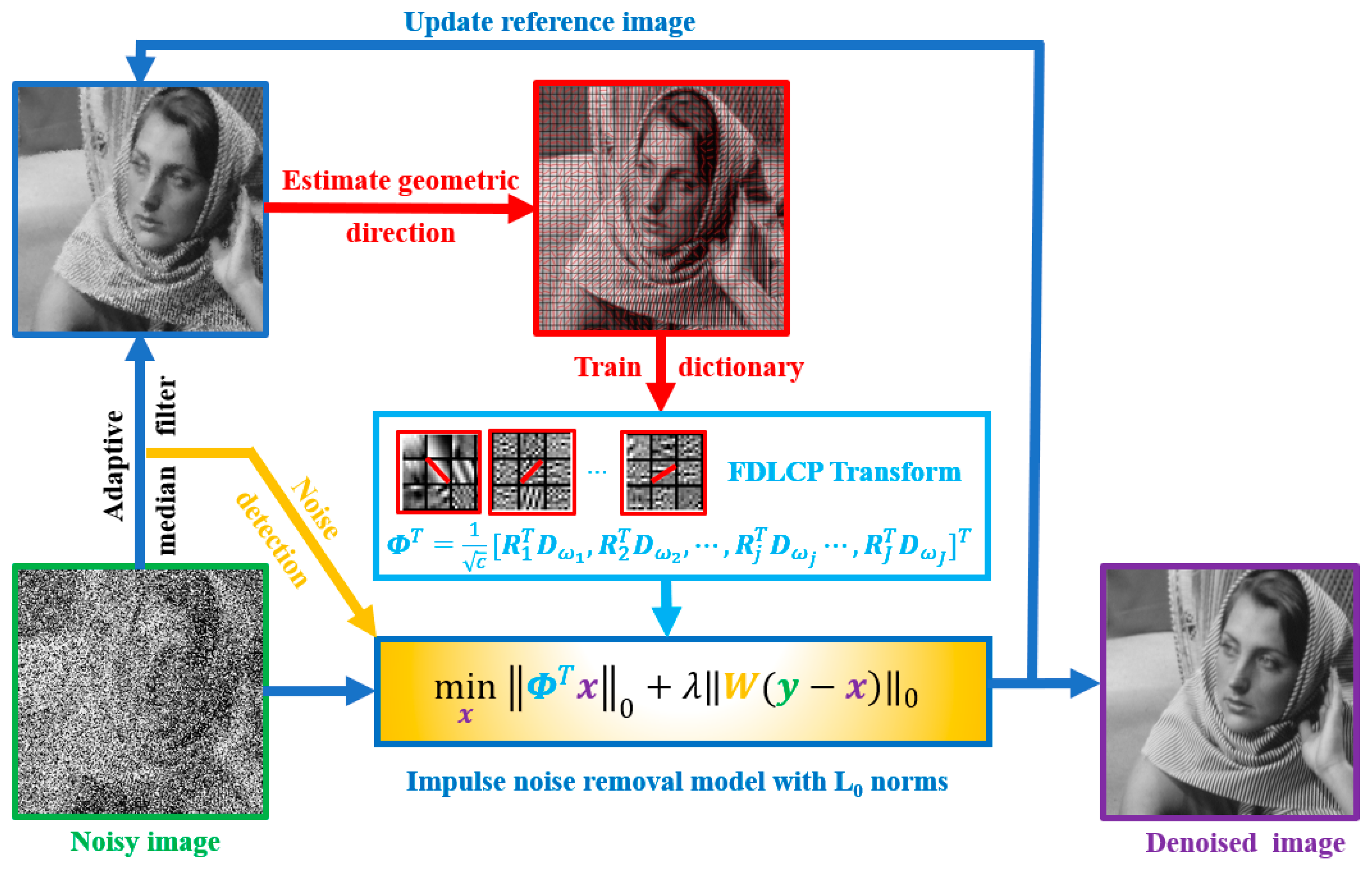
2.2. Proposed Method

In this work, we propose an approach to remove the impulse noise with fast adaptive dictionary learning to provide sparsity of images and formulate the denoising problems with the L0 norms regularizations.
The flowchart of the whole scheme is summarized in Figure 1. First, a reference image is initially obtained from a noised image using the AMF. Then, the geometric directions are learnt from the reference image to get the adaptive sparse transform is via fast dictionary training. Next, a denoised image is reconstructed using the proposed L0 norms regularization model.
In the following, the essential part of the approach will be given in more details.

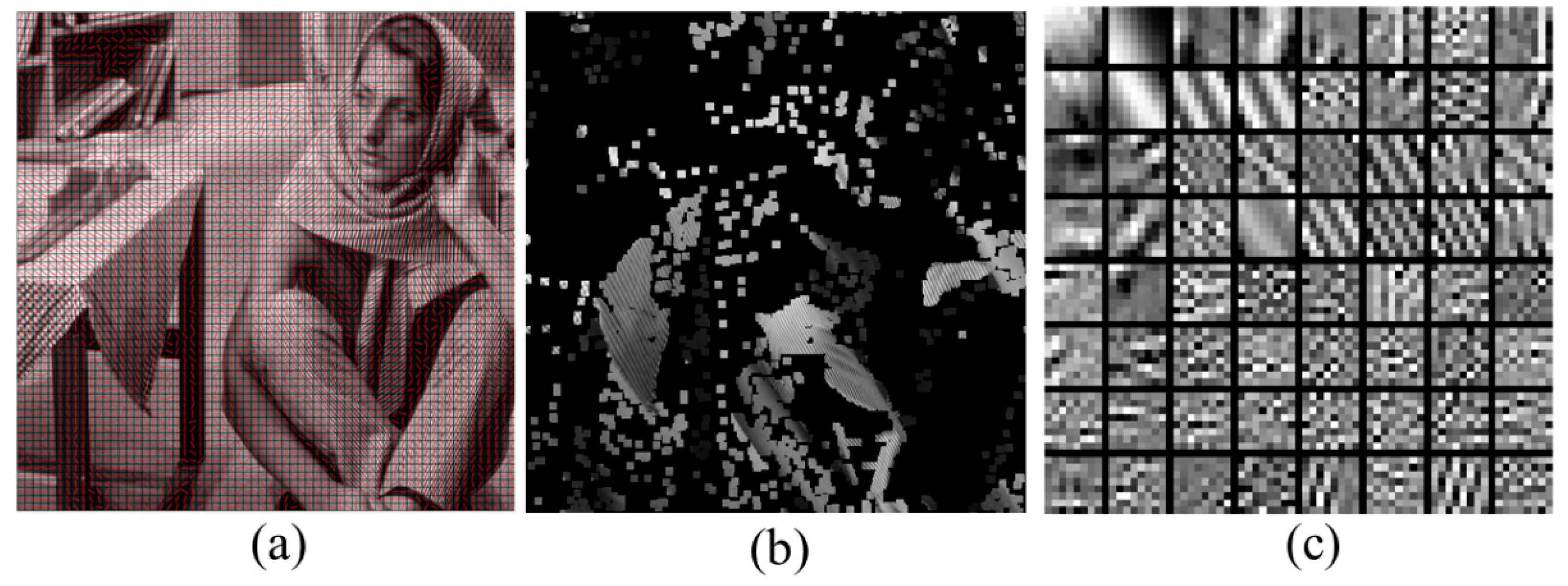
2.2.1. Adaptive Dictionary Learning in Salt and Pepper Noise Removal

We first introduce the Fast Dictionaries Learning Method on Classified Patches (FDLCP) [13] into salt and pepper noise removal. FDLCP not only inherits fast learning to form orthogonal dictionaries, but also provides sparser representations by training comprehensive dictionaries for different geometrical image patches. As shown in Figure 2, patches that share the same geometric direction are grouped together to form one class, and then this class is used to learn a specific dictionary. Therefore, the dictionary of each class effectively captures the underlying image structures (Figure 2c).
Mathematically, within a class of patches X ω that shares a same geometric direction ω , an orthogonal dictionary is trained by solving the optimization problem [15]:
min D ω , Z   X ω D ω Z F 2 + η 2 Z 0 s . t . D ω T D ω = I
where D w is the dictionary and . F is the Frobenius norm. We choose the orthogonal dictionary learning because it enables the significant reduction of computation [13,15] than the commonly redundant dictionary trained in the K-SVD. For example, it has been shown that the computational time of learning orthogonal dictionary will be approximately 1% than that of the redundant dictionary in K-SVD [13].
Equation (3) can be fast solved by alternatively computing the sparse coding Z and updating the dictionary D ω in each iteration [13,15] as follows:
(1) Given the current dictionary D ω , update sparse coefficients Z via hard thresholding:
Z = H c ( D ω T X ω )
where the hard threshold H c ( Q ) for a matrix Q is an element-wise operator that performs on the element Q i j according to H c ( Q i j ) = { 0 ,   i f   a b s ( Q i j ) c Q i j , i f   a b s ( Q i j ) > c with a threshold c.
(2) Given the coefficients Z , compute dictionary D ω according to:
min D ω X ω D ω Z F 2 s . t . D ω T D ω = I ,
where η is a parameter to decide the sparsity and I is an identity matrix. The solution of Equation (5) is:
D ω = P V T ,
where P and V are orthogonal matrices of the following singular value decomposition:
X ω Z T = P Λ V T ,
where T denotes the matrix transpose. The solutions in Equations (7) and (8) are called the orthogonal Procrustes solutions, which were first considered in dictionary learning before [35]. In our implementation, the parameter η is set to 0.2 in all experiments.
A good feature of the FDLCP [15] is that it balances the fast learning via orthogonal dictionary, comparing with the relatively slow learning in the classic K-SVD [12], and sparse representation for each classes, comparing with the sole orthogonal dictionary for all image patches [13]. FDLCP has been observed to outperform K-SVD in the medical image reconstruction [15], but not yet applied to impulse denoise so far.
To further derive the mathematical property of FDLCP, let R j denote the operator that extract a patch owned with jth geometric direction from an image x , and then the FDLCP transform is simplified as Ψ T = [ R 1 T D ω 1 , R 2 T D ω 2 , , R j T D ω j , R J T D ω J ] T for the total J geometric directions. The forward and inverse transform satisfies:
Ψ T Ψ = [ R 1 T D ω 1 , R 2 T D ω 2 , , R J T D ω J ] T [ R 1 T D ω 1 , R 2 T D ω 2 , , R J T D ω J ] =   c I ,
where I is an identity matrix and the variable c is the overlapping factor for image patches [15]. By further setting Φ T = 1 c Ψ T , the transform Φ obeys:
Φ Φ T = I ,
meaning that the modified FDLCP transform Φ is a tight frame for image reconstruction [36].
Then, how to train the representations with FDLCP in the salt and pepper noise removal? We suggest learning the FDLCP from a reasonable pre-reconstructed image, e.g., which is obtained with AMF. This strategy has been found to achieve sparse representations under fast computing not only in impulse noise removal [10,11], but also other image reconstruction problems [15,16,37].

2.2.2. FLCLP-Based Image Reconstruction with The L0 Norm Regularizations

Two L1 norm terms are defined in Equation (2) for impulse noise removal, and they play different roles and can be replaced by two L0 norms for a better reconstruction. The first term enforces the image sparsity, and the L1 norm may lose weak signals in the reconstruction, thus, researchers tend to minimize the sparsity by the L0 norm. This modification has been observed to improve the reconstruction [8,15,20,21] including impulse denoise removal [18]. The second term maintains the data fidelity, and L1 norm may reduce robustness to impulse noise [6,29,30], while using the L0 norm has been observed to significantly improve rejecting the outliers and good edge preserving in the reconstruction [18]. Therefore, both the L0 norm terms on the sparsity and data fidelity are adopted in this work.
The FLCLP-based image reconstruction with the L0 norm regularizations is proposed as follows:
min x   Φ T x 0 + λ W ( y x ) 0
where the α 0 is the total number of nonzero entries in the α . For simplicity, we name the proposed method as FDLCP-L0 in the following descriptions. The two L0 norms significantly boost the FDLCP-based impulse noise removal as shown in Figure 3.
To better understand the model, we will illustrate L0 norm regularizations from the Bayesian view.
Given the observed noisy image y , the maximize posterior probability for the reconstructed image x can be obtained by maximize posterior probability:
m a x x { log p ( y | x ) + log p ( x ) } .
Since a given x corresponds to the unique transform coefficients Φ T x , then p ( y | Φ T x ) = p ( y | x ) . By plugging in the salt and pepper noise model:
y j = { 0 ,   with   probability   q 2 1 ,   with   probability   q 2 x j ,   with   probability   1 q
where q is the probability that jth pixel is contaminated by noise, then the first term in Equation (11) is modified as [18]:
p ( y | x ) = e 1 q = 1 y x 0 N
Therefore, ignoring the constant in Equation (13), maximizing the posterior probability of x means minimizing y x 0 , which is the same as our data consistency term in Equation (10) by setting W as the identity matrix.
We then use a transform domain prior as p ( x ) = 1 v e g [ Φ T x ] where α = Φ T x and g ( α j ) = { 1 h ,   if   α j = 0 h ,   otherwise and h is a probability of a coefficient being in nonzero value. Then, maximizing the log function of p ( x ) leads to minimizing Φ T x 0 which is the same as our sparsity constraint term.
The above analysis implies that the L0 norm in data consistency specifically works for impulse noise removal, and the L0 norm that directly counts the number of non-zero coefficients in sparsity constraint evaluates the sparsity better the L1 norm.

2.2.3. Numerical Algorithm

Directly solving Equation (10) is very hard since its L0 norm terms are non-smooth and non-differential. In this work, we adopt the alternating direction minimization with continuation algorithm (ADMC) [10,16,37] to solve Equation (10). ADMC is chosen since it enables to obtain the solution with much easier sub-problems that have analytical solutions as discussed below.
By introducing the continuation parameter β and augmented variables α and d , a relax form of Equation (10) is:
min α , d , x ( α 0 + β 2 α Φ T x 2 2 ) + λ ( d 0 + β 2 d W ( y x ) 2 2 )
where α and d are two augmented variables. When β , the solution of Equation (14) approaches that of Equation (10) since any non-zero values of α Φ T x (or d W ( y x ) ) will lead β 2 α Φ T x 2 2 (or β 2 d W ( y x ) 2 2 ) to be infinite. Therefore, in order to minimize the cost function of Equation (14), both α = Φ T x and d = W ( y x ) must be simultaneously satisfied, meaning that Equation (14) is equivalent to Equation (10) when β . In the implementation, we gradually increase β .
While β is fixed at the kth iterations, the solution of Equation (14) is obtained by alternatively solving the following sub-problems where each one has the analytical solution.
(1) Fixed d ( k ) and x ( k ) , solve:
α ( k + 1 ) = arg min α α 0 + β 2 α Φ T x ( k ) 2 2 ,
whose solution is achieved by hard thresholding according to:
α ( k + 1 ) = H 2 β ( Φ T x ) .
(2) Fix x ( k ) and α ( k + 1 ) , solve:
d ( k + 1 ) = arg min d d 0 + β 2 d W ( y x ( k ) ) 2 2 ,
whose solution is also achieved by hard thresholding as follows
d ( k + 1 ) = H 2 β ( W ( y x ( k ) ) )
(3) Fix α ( k + 1 ) and d ( k + 1 ) , solve:
x ( k + 1 ) = arg min x α ( k + 1 ) Φ T x 2 2 + λ d ( k + 1 ) W ( y x ) 2 2 ,
and have the solution as follows:
x ( k + 1 ) = ( I + λ W T W ) 1 ( Φ α ( k + 1 ) + λ W T ( W y d ( k + 1 ) ) ) .
The algorithm is summarized in Algorithm 1. It is worth noting that the existing ADMC algorithms solve either a reconstruction model with minimization of L1 norm (sparsity regularization) and L2 norm (data fidelity) in compressive image recovery [16,38,39], or a denoising model with minimization of L1 norm (sparsity regularization) and L1 norm (data fidelity) for impulse noise removal [10,11]. The ADMC algorithm derived in the work solves the denoising model with minimization of L0 norm (sparsity regularization) and L0 norm (data consistency) as Equation (14) and has totally different sub-problems and solutions from previous ones.
Algorithm 1. ADMC Algorithm for the L0 Norm Minimizations.
Input: The noise image y , diagonal matrix W , adaptive dictionaries Φ , and the regularization λ
Initialize: β = 1 , β m a x = 2 10 , k = 1, and x ( 1 ) = y .
Main:
While β β m a x , repeat steps (a)~(d) until convergence:
(a) Update α ( k + 1 ) by computing α ( k + 1 ) = H 2 β , ( Φ T x ( k ) ) ( H c ( ) denotes the hard thresholding operator with a threshold c [20].) according to Equation (16).
(b) Update d ( k + 1 ) by solving d ( k + 1 ) = H 2 β ( W ( y x ( k ) ) ) according to Equation (18).
(c) Compute x ( k + 1 ) via Equation (20).
(d) Evaluate the difference of successive reconstruction ξ = x ( k + 1 ) x ( k ) 2 x ( k ) 2 ,
(e) If ξ > 10 4 , go to (a); else set β 2 β and k k + 1 .
End While
Output: Reconstructed image x .

3. Results

The proposed method, FDLCP-L0, is compared with basic AMF [2], the state-of-the-art PANO-L1 [9] and total variation (TV)-L0 methods [17]. Two objective evaluation criteria, the peak signal-to-noise ratio (PSNR) and the mean measure of structural similarity (MSSIM) [40], which are most widely used in image denoising and reconstruction [15,17,37,41,42], are adopted to quantitatively measure the denoising performance here. The PSNR measures average pixel distortion of the denoised image and the MSSIM specifically cares about the preserved image structures, e.g., local luminance and contrast, which are important for human visual systems [40]. Higher PSNR and MSSIM mean better denoising performance. All the computations were performed on four cores 3.6 GHz CPU desktop computer with 16 GB RAM. The typical reconstruction time of a 512 × 512 image with AMF, PANO-L1, TV-L0, and FDLCP-L0 are 0.25 s, 55.7 s, 6.74 s, and 473.22 s, respectively. The test images are downloaded from website [43].

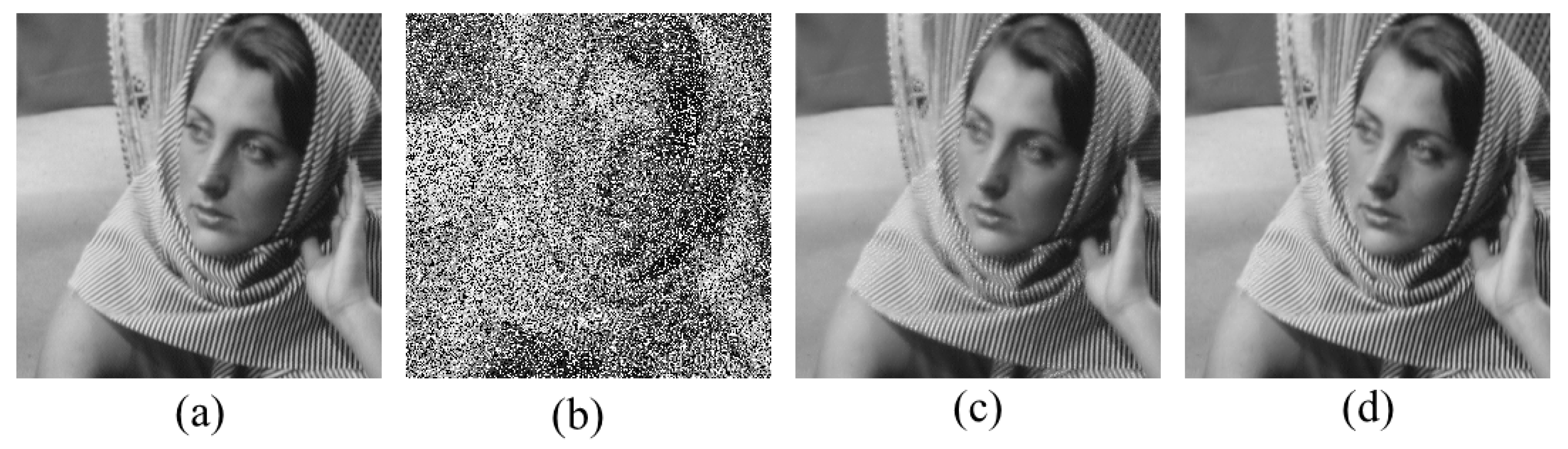
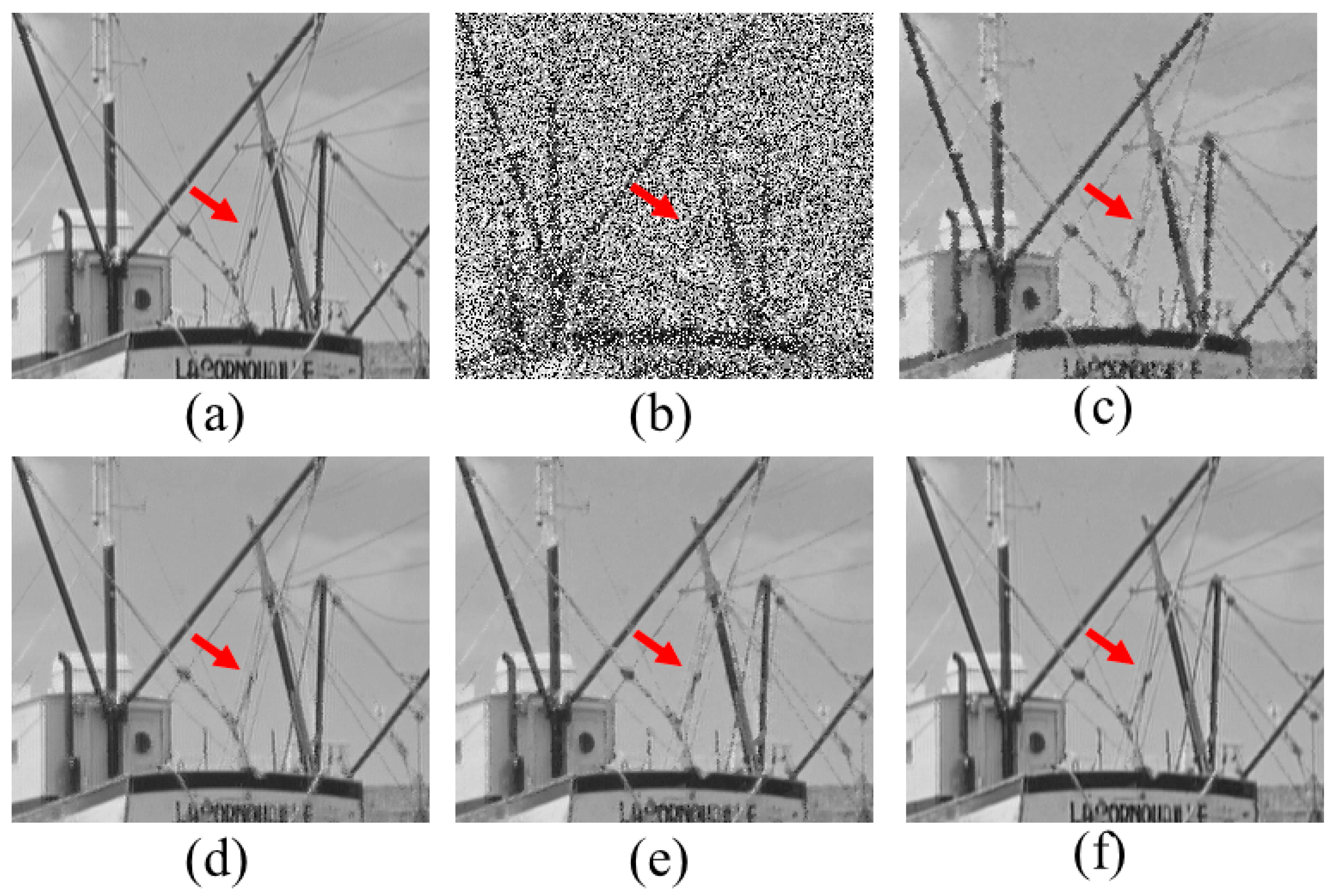
3.1. Denoising Performance under a Fixed Noise Level

At the typical noise level of 0.5 (50% pixels are contaminated by salt and pepper noise), both PANO-L1 and TV-L0 remove noise much better than the classic AMF. However, the two state-of-the-art approaches still lose some straight lines (Figure 4d,e) or weaken some textures (Figure 5d,e). The proposed method reconstructs these image features much better than others. As listed in Table 1, evaluation criteria including both PSNR and MSSIM indicate that the proposed method reconstructs the most consistent images to the noise-free ones.

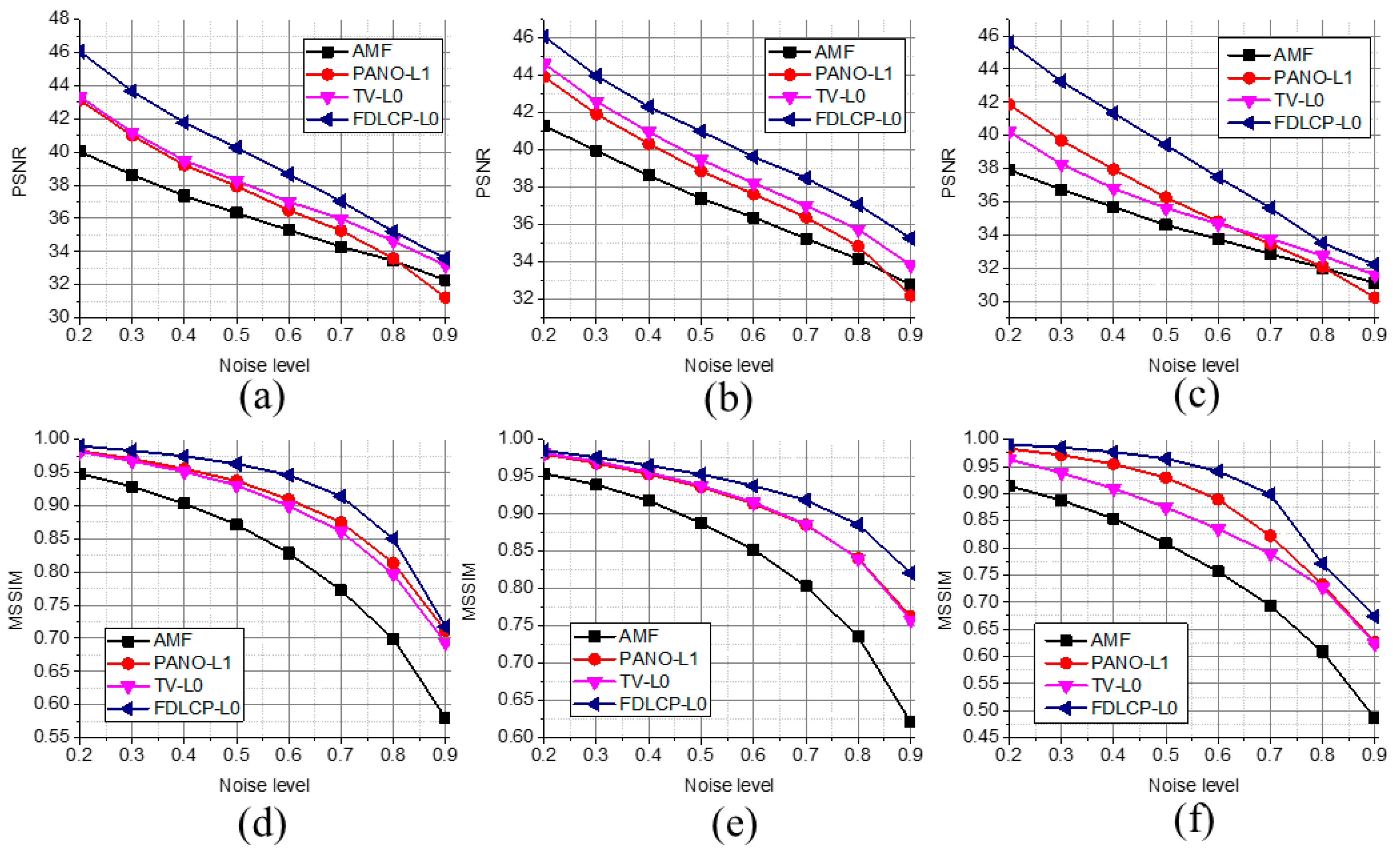
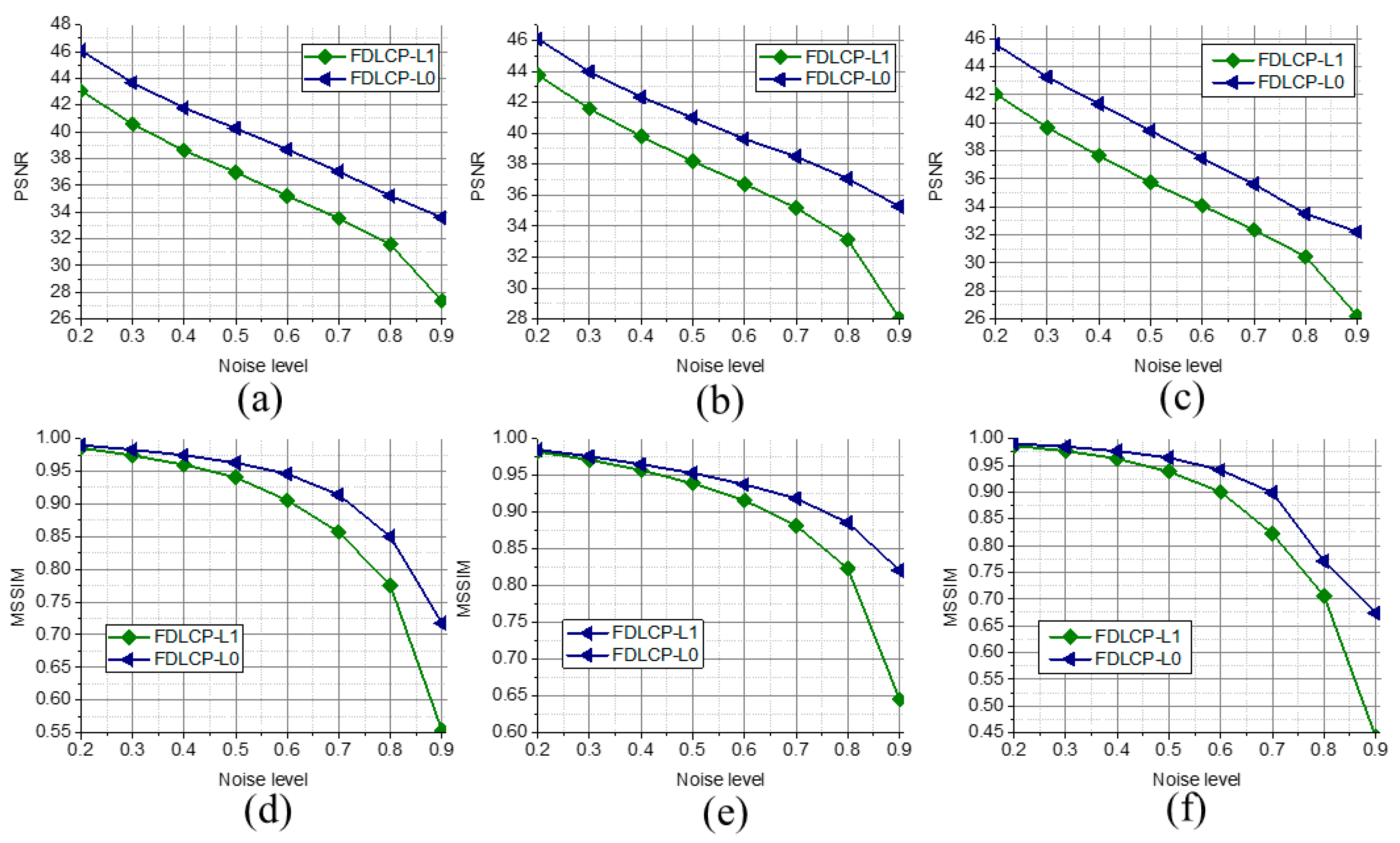
3.2. Denoising Performance under Different Noise Levels

The denoising performances under different noise levels were evaluated in Figure 6. The AMF is inferior to other compared methods. The TV-L0 outperforms the PANO-L1 although PANO provides adaptive sparse representation. This observation implies that the L0 norm is more robust than the L1 norm to the outliers introduced by the impulse noise. The proposed method not only makes use of adaptive sparsity in the representation but also incorporates the robust L0 norm to better remove outliers in the data fidelity term. Therefore, improved denoising performance by the proposed method are consistently observed in all experiments with different noise levels.

4. Discussions

To further confirm the advantage of using the L0 norm over the L1 norm, FDLCP-L1 is compared with the proposed method FDLCP-L0. Typical denoised images are shown in Figure 7 and quantitative measures are shown Figure 8, Table 2 and Table 3. Image features are preserved much better using FDLCP-L0 than that using FDLCP-L1. Consistent improvements at all noise levels are observed for FDLCP-L0. Therefore, replacing the L1 norm with the L0 norm is valuable to improve the quality of the images that are contaminated by the salt and pepper noise.

5. Conclusions

A new salt and pepper impulse noise removal method is proposed by simultaneously exploring: (1) The adaptively sparse representation of images; (2) better regularizing the sparsity of representation and the data fidelity under impulse noise. The former is accomplished via fast orthogonal dictionary learning within multiclass geometric image patches while the latter is enforced by regularizing L0 norms on both the sparsity and data fidelity constraints. Experimental results demonstrate that this proposed approach outperforms the compared ones in terms of better preserving image structures and higher objective denoising performance evaluation criteria. The theoretical prof of the advantage of L0 norm over L1 norm in impulse noise removal would be an interesting future work.

Author Contributions

Conceptualization, D.G.; Data curation, Z.T. and J.W.; Formal analysis, Z.T. and J.W.; Funding acquisition, D.G. and X.Q.; Investigation, D.G. and X.D.; Methodology, D.G.; Project administration, D.G.; Resources, M.X.; Software, J.W.; Supervision, X.Q.; Writing—original draft, D.G.; Writing—review & editing, D.G., Z.T., X.D. and X.Q.

Funding

This work was supported in part by National Natural Science Foundation of China (No. 61871341, 61672335, and 61601276), the Science and Technology Program of Xiamen (No. 3502Z20183053), the Natural Science Foundation of Fujian Province of China (No. 2016J05205 and 2018J06018), the Fundamental Research Funds for the Central Universities (No. 20720180056).

Acknowledgments

Di Guo is grateful to Ming-Ting Sun for hosting the visit at University of Washington when writing this work and China Scholarship Council (No. 201808350010) to support the visit.

Conflicts of Interest

The authors declare that there is no conflict of interests regarding the publication of this article.

References

  1. Gonzalez, R.C.; Richard, E. Digital Image Processing; Prentice Hall Press: Upper Saddle River, NJ, USA, 2002. [Google Scholar]
  2. Hwang, H.; Haddad, R. Adaptive median filters: New algorithms and results. IEEE Trans. Image Process. 1995, 4, 499–502. [Google Scholar] [CrossRef] [PubMed]
  3. Sree, P.S.J.; Kumar, P.; Siddavatam, R.; Verma, R. Salt-and-pepper noise removal by adaptive median-based lifting filter using second-generation wavelets. Signal Image Video Process. 2013, 7, 111–118. [Google Scholar] [CrossRef]
  4. Adeli, A.; Tajeripoor, F.; Zomorodian, M.J.; Neshat, M. Comparison of the Fuzzy-based wavelet shrinkage image denoising techniques. Int. J. Comput. Sci. 2012, 9, 211–216. [Google Scholar]
  5. Mafi, M.; Martin, H.; Cabrerizo, M.; Andrian, J.; Barreto, A.; Adjouadi, M. A comprehensive survey on impulse and Gaussian denoising filters for digital images. Signal Process. 2018. [Google Scholar] [CrossRef]
  6. Huang, S.; Zhu, J. Removal of salt-and-pepper noise based on compressed sensing. Electron. Lett. 2010, 46, 1198–1199. [Google Scholar] [CrossRef]
  7. Wang, X.-L.; Wang, C.-L.; Zhu, J.-B.; Liang, D.-N. Salt-and-pepper noise removal based on image sparse representation. Opt. Eng. 2011, 50, 097007. [Google Scholar] [CrossRef]
  8. Xiao, Y.; Zeng, T.; Yu, J.; Ng, M.K. Restoration of images corrupted by mixed Gaussian-impulse noise via l1–l0 minimization. Pattern Recognit. 2011, 44, 1708–1720. [Google Scholar] [CrossRef]
  9. Wang, S.; Liu, Q.; Xia, Y.; Dong, P.; Luo, J.; Huang, Q.; Feng, D.D. Dictionary learning based impulse noise removal via L1–L1 minimization. Signal Process. 2013, 93, 2696–2708. [Google Scholar] [CrossRef]
  10. Guo, D.; Qu, X.; Du, X.; Wu, K.; Chen, X. Salt and pepper noise removal with noise detection and a patch-based sparse representation. Adv. Multimed. 2014, 2014. [Google Scholar] [CrossRef]
  11. Guo, D.; Qu, X.; Wu, M.; Wu, K. A modified iterative alternating direction minimization algorithm for impulse noise removal in images. J. Appl. Math. 2014, 2014, 595782. [Google Scholar] [CrossRef]
  12. Aharon, M.; Elad, M.; Bruckstein, A. K-SVD: An algorithm for designing overcomplete dictionaries for sparse representation. IEEE Trans. Signal Process. 2006, 54, 4311–4322. [Google Scholar] [CrossRef]
  13. Cai, J.-F.; Ji, H.; Shen, Z.; Ye, G.-B. Data-driven tight frame construction and image denoising. Appl. Comput. Harmonic Anal. 2014, 37, 89–105. [Google Scholar] [CrossRef]
  14. Ravishankar, S.; Bresler, Y. MR image reconstruction from highly undersampled k-space data by dictionary learning. IEEE Trans. Med. Imaging 2011, 30, 1028–1041. [Google Scholar] [CrossRef] [PubMed]
  15. Zhan, Z.; Cai, J.F.; Guo, D.; Liu, Y.; Chen, Z.; Qu, X. Fast multiclass dictionaries learning with geometrical directions in MRI reconstruction. IEEE Trans. Biomed. Eng. 2016, 63, 1850–1861. [Google Scholar] [CrossRef] [PubMed]
  16. Qu, X.; Hou, Y.; Lam, F.; Guo, D.; Zhong, J.; Chen, Z. Magnetic resonance image reconstruction from undersampled measurements using a patch-based nonlocal operator. Med. Image Anal. 2014, 18, 843–856. [Google Scholar] [CrossRef] [PubMed]
  17. Dabov, K.; Foi, A.; Katkovnik, V.; Egiazarian, K. Image denoising by sparse 3-D transform-domain collaborative filtering. IEEE Trans. Image Process. 2007, 16, 2080–2095. [Google Scholar] [CrossRef] [PubMed]
  18. Ganzhao, Y.; Ghanem, B. L0TV: A new method for image restoration in the presence of impulse noise. In Proceedings of the IEEE Conference on Computer Vision and Pattern Recognition-CVPR 2015, Boston, MA, USA, 7–12 June 2015; pp. 5369–5377. [Google Scholar]
  19. Trzasko, J.; Manduca, A. Highly undersampled magnetic resonance image reconstruction via homotopic L0-minimization. IEEE Trans. Med. Imaging 2009, 28, 106–121. [Google Scholar] [CrossRef]
  20. Ning, B.; Qu, X.; Guo, D.; Hu, C.; Chen, Z. Magnetic resonance image reconstruction using trained geometric directions in 2D redundant wavelets domain and non-convex optimization. Magn. Reson. Imaging 2013, 31, 1611–1622. [Google Scholar] [CrossRef]
  21. Qu, X.; Cao, X.; Guo, D.; Hu, C.; Chen, Z. Compressed sensing MRI with combined sparsifying transforms and smoothed L0 norm minimization. In Proceedings of the IEEE International Conference on Acoustics, Speech and Signal Processing-ICASSP 2010, Dallas, TX, USA, 14–19 March 2010; pp. 626–629. [Google Scholar]
  22. Qu, X.; Qiu, T.; Guo, D.; Lu, H.; Ying, J.; Shen, M.; Hu, B.; Orekhov, V.; Chen, Z. High-fidelity spectroscopy reconstruction in accelerated NMR. Chem. Commun. 2018, 54, 10958–10961. [Google Scholar] [CrossRef]
  23. Qu, X.; Guo, D.; Cao, X.; Cai, S.; Chen, Z. Reconstruction of self-sparse 2D NMR spectra from undersampled data in the indirect dimension. Sensors 2011, 11, 8888–8909. [Google Scholar] [CrossRef]
  24. Qu, X.; Cao, X.; Guo, D.; Chen, Z. Compressed sensing for sparse magnetic resonance spectroscopy. In Proceedings of the 18th Scientific Meeting on International Society for Magnetic Resonance in Medicine-ISMRM 2010, Stockholm, Sweden, 1–7 May 2010; p. 3371. [Google Scholar]
  25. Li, Q.; Liang, S. Weak fault detection of tapered rolling bearing based on penalty regularization approach. Algorithms 2018, 11, 184. [Google Scholar] [CrossRef]
  26. Zhu, Z.; Yin, H.; Chai, Y.; Li, Y.; Qi, G. A novel multi-modality image fusion method based on image decomposition and sparse representation. Inf. Sci. 2018, 432, 516–529. [Google Scholar] [CrossRef]
  27. Zhu, Z.; Qi, G.; Chai, Y.; Chen, Y. A novel multi-focus image fusion method based on stochastic coordinate coding and local density peaks clustering. Future Internet 2016, 8, 53. [Google Scholar] [CrossRef]
  28. Qi, G.; Zhu, Z.; Chen, Y.; Wang, J.; Zhang, Q.; Zeng, F. Morphology-based visible-infrared image fusion framework for smart city. Int. J. Simul. Process Modell. 2018, 13, 523–536. [Google Scholar] [CrossRef]
  29. Nikolova, M. A variational approach to remove outliers and impulse noise. J. Math. Imaging Vis. 2004, 20, 99–120. [Google Scholar] [CrossRef]
  30. Cai, J.-F.; Chan, R.; Nikolova, M. Fast two-phase image deblurring under impulse noise. J. Math. Imaging Vis. 2010, 36, 46–53. [Google Scholar] [CrossRef]
  31. Huang, J.; Zhang, T. The benefit of group sparsity. Ann. Stat. 2010, 38, 1978–2004. [Google Scholar] [CrossRef]
  32. Wang, L.; Chen, Y.; Lin, F.; Chen, Y.; Yu, F.; Cai, Z. Impulse noise denoising using total variation with overlapping group sparsity and Lp-pseudo-norm shrinkage. Appl. Sci. 2018, 8, 2317. [Google Scholar] [CrossRef]
  33. Chen, P.; Selesnick, I.W. Group-sparse signal denoising: Non-convex regularization, convex optimization. IEEE Trans. Signal Process. 2014, 62, 3464–3478. [Google Scholar] [CrossRef]
  34. Alpago, D.; Zorzi, M.; Ferrante, A. Identification of sparse reciprocal graphical models. IEEE Control Syst. Lett. 2018, 2, 659–664. [Google Scholar] [CrossRef]
  35. Lesage, S.; Gribonval, R.; Bimbot, F.; Benaroya, L. Learning unions of orthonormal bases with thresholded singular value decomposition. In Proceedings of the IEEE International Conference on Acoustics, Speech, and Signal Processing-ICASSP′05, Philadelphia, PA, USA, 18–23 March 2005; Volume 5, pp. 293–296. [Google Scholar]
  36. Liu, Y.; Zhan, Z.; Cai, J.F.; Guo, D.; Chen, Z.; Qu, X. Projected iterative soft-thresholding algorithm for tight frames in compressed sensing magnetic resonance imaging. IEEE Trans. Med. Imaging 2016, 35, 2130–2140. [Google Scholar] [CrossRef] [PubMed]
  37. Lai, Z.; Qu, X.; Liu, Y.; Guo, D.; Ye, J.; Zhan, Z.; Chen, Z. Image reconstruction of compressed sensing MRI using graph-based redundant wavelet transform. Med. Image Anal. 2016, 27, 93–104. [Google Scholar] [CrossRef] [PubMed]
  38. Yang, J.; Zhang, Y.; Yin, W. A fast TVL1-L2 Minimization Algorithm for Signal Reconstruction from Partial Fourier Data. Rice University. 2009. Available online: ftp://ftp.math.ucla.edu/pub/camreport/cam09-24.pdf (accessed on 1 October 2018).
  39. Yang, J.; Zhang, Y.; Yin, W. A fast alternating direction method for TV l1-l2 signal reconstruction from partial fourier data. IEEE J. Sel. Top. Signal Process. 2010, 4, 288–297. [Google Scholar] [CrossRef]
  40. Zhou, W.; Bovik, A.C.; Sheikh, H.R.; Simoncelli, E.P. Image quality assessment: From error visibility to structural similarity. IEEE Trans. Image Process. 2004, 13, 600–612. [Google Scholar]
  41. Portilla, J.; Strela, V.; Wainwright, M.J.; Simoncelli, E.P. Image denoising using scale mixtures of Gaussians in the wavelet domain. IEEE Trans. Image Process. 2003, 12, 1338–1351. [Google Scholar] [CrossRef] [PubMed]
  42. Elad, M.; Aharon, M. Image denoising via sparse and redundant representations over learned dictionaries. IEEE Trans. Image Process. 2006, 15, 3736–3745. [Google Scholar] [CrossRef] [PubMed]
  43. Computational Imaging and Visual Image Processing. Available online: http://www.io.csic.es/PagsPers/JPortilla/image-processing/bls-gsm/63-test-images (accessed on 1 October 2018).
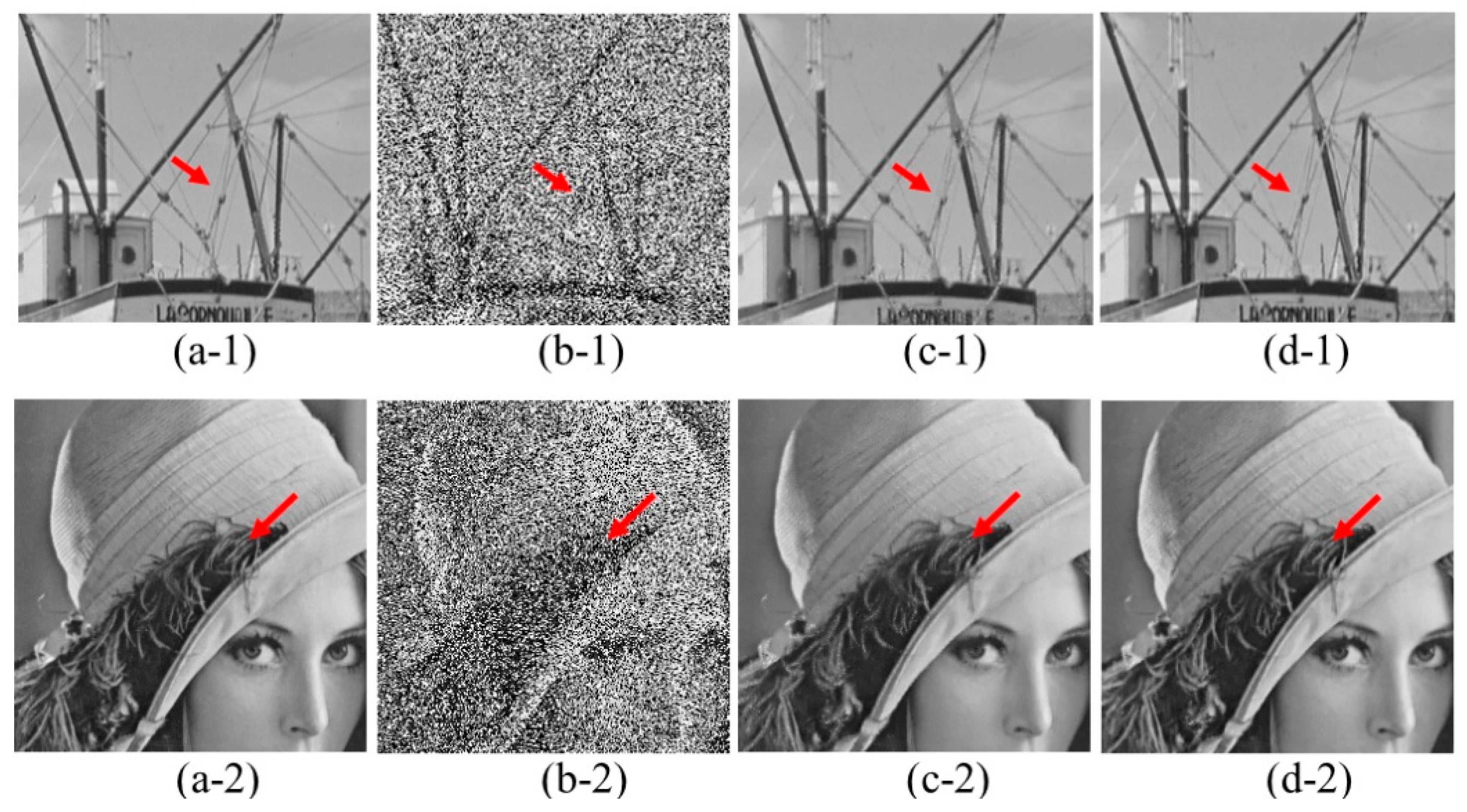
Figure 1. A flowchart of the proposed method on impulse noise removal.
Algorithms 12 00007 g001
Figure 2. Adaptive representations learnt with FDLCP. (a) Geometric directions estimated from the Barbara image, (b) one class of image patches that share the same geometric direction, (c) one dictionary learnt from the class of patches in (b). Note: red lines in (a) indicate geometric directions of image patches.
Algorithms 12 00007 g002
Figure 3. Comparisons on the denoised Barbara images using different norms. (a) is the noise-free image, (b) is the noisy image, (c) and (d) are denoised images using FDLCP with L1 and L0 norm minimizations, respectively. Note: The noise level is 0.5, meaning that 50% pixels are contaminated by salt and pepper noise.
Algorithms 12 00007 g003
Figure 4. Denoised boat images at the noise level of 0.5. (a) is the noise-free image, (b) is the noisy image, (c)–(f) are denoised images using AMF, PANO-L1, TV-L0, and the proposed FDLCP-L0, respectively.
Algorithms 12 00007 g004
Figure 5. Denoised Lena images at the noise level of 0.5. (a) is the noise-free image, (b) is the noisy image, (c)–(f) are denoised images using AMF, PANO-L1, TV-L0, and the proposed FDLCP-L0, respectively.
Algorithms 12 00007 g005
Figure 6. Quantitative measure at different noise levels. (a)–(c) are PSNRs of Boat, Lena, and Barbara images, respectively; (d)–(f) are MSSIMs of Boat, Lena, and Barbara images, respectively.
Algorithms 12 00007 g006
Figure 7. Comparisons on denoised images using FDLCP-L1 and FDLCP-L0. (a) and (b) are noise-free and noisy images, (c) and (d) are denoised images using FDLCP-L1 and FDLCP-L0, respectively. The first row and the second row are Boat and Lena images. Note: The salt and pepper noise level is 0.5 and the denoised Barbara images is shown in Figure 3.
Algorithms 12 00007 g007
Figure 8. Comparisons on quantitative measure using FDLCP-L1 and FDLCP-L0. (a)–(c) are PSNRs of Boat, Lena, and Barbara images, respectively; (d)–(f) are MSSIMs of Boat, Lena, and Barbara images, respectively.
Algorithms 12 00007 g008
Table 1. Quantitative measures at the salt and pepper impulse noise level of 0.5.
ImagesQuantitative MeasureMethods
AMFPANO-L1TV-L0FDLCP-L0
BoatPSNR36.3237.9538.2940.26
MSSIM0.87150.93750.93070.9631
LenaPSNR37.4238.8739.4841.01
MSSIM0.88780.93600.93820.9531
BarbaraPSNR34.6136.2835.6339.44
MSSIM0.80800.92930.87460.9644
Table 2. PSNR performance under the salt and pepper noise using FDCLP with L1 or L0 norms.
ImagesMethodsNoise Level
0.20.30.40.50.60.70.80.9
BoatL143.0740.5838.6036.9935.2033.5431.5827.35
L046.0743.6841.7840.2638.6737.0435.2133.59
LenaL143.7541.5839.8038.1736.7135.1833.1228.04
L046.0943.9742.3241.0139.6338.4937.0735.27
BarbaraL142.0639.6737.6535.7434.0832.3830.4526.21
L045.6243.2741.3539.4437.4835.6333.5232.22
Table 3. MSSIM performance under the salt and pepper noise using FDCLP with L1 or L0 norms.
ImagesMethodsNoise Level
0.20.30.40.50.60.70.80.9
BoatL10.98560.97430.96010.94070.90550.85710.77520.5537
L00.99000.98300.97450.96310.94610.91390.85010.7178
LenaL10.98220.97110.95690.93910.91590.88190.82320.6458
L00.98490.97590.96500.95310.93760.91880.88560.8208
BarbaraL10.98670.97690.96240.93850.90010.82200.70580.4427
L00.99090.98490.97660.96440.94120.89870.77090.6736

