Article

Steady-State Performance of an Adaptive Combined MISO Filter Using the Multichannel Affine Projection Algorithm

by
Danilo Comminiello
1,*,
Michele Scarpiniti
1,
Luis A. Azpicueta-Ruiz
2 and
Aurelio Uncini
1
1
Department of Information Engineering, Electronics and Telecommunications (DIET), Sapienza University of Rome, 00185 Roma RM, Italy
2
Department of Signal Theory and Communications, Universidad Carlos III de Madrid, 28903 Getafe, Spain
*
Author to whom correspondence should be addressed.
Algorithms 2019, 12(1), 2; https://doi.org/10.3390/a12010002
Submission received: 3 December 2018 / Revised: 12 December 2018 / Accepted: 14 December 2018 / Published: 20 December 2018
(This article belongs to the Special Issue Adaptive Filtering Algorithms)

Abstract

:
The combination of adaptive filters is an effective approach to improve filtering performance. In this paper, we investigate the performance of an adaptive combined scheme between two adaptive multiple-input single-output (MISO) filters, which can be easily extended to the case of multiple outputs. In order to generalize the analysis, we consider the multichannel affine projection algorithm (APA) to update the coefficients of the MISO filters, which increases the possibility of exploiting the capabilities of the filtering scheme. Using energy conservation relations, we derive a theoretical behavior of the proposed adaptive combination scheme at steady state. Such analysis entails some further theoretical insights with respect to the single channel combination scheme. Simulation results prove both the validity of the theoretical steady-state analysis and the effectiveness of the proposed combined scheme.

1. Introduction

The convergence performance of an adaptive filtering is decisively affected by the choice of certain characteristic parameters of the filter. This is one of the main motivations behind the high number of adaptive algorithms and structures that are continually introduced in the literature to provide improvements of convergence and steady-state performance in certain scenarios. The design of an adaptive filter may be even very risky when no a priori information is provided on the model of the signal to be processed. One solution to this problem is represented by the adaptive combination of adaptive filters [1,2,3,4,5,6], which exploits the diversity of parallel adaptive branches. Combined structures of filtering have been applied to a wide variety of online adaptive filtering applications [7,8,9,10,11,12,13,14,15] due to their capabilities of detecting and selecting instant by instant the best-performing filter. To this end, the analysis of the mean squared performance aims at showing the effectiveness of adaptive combined schemes and how to exploit them the best [6,16,17,18,19,20].
In this paper, we focus on the combination of adaptive filters in the multichannel case. In particular, the combined structure that we take into account is composed of a convex combination of two adaptive multiple-input single-output (MISO) filters [8]. MISO filters are widely used in several applications, such as adaptive beamforming [21,22], OFDM systems [23], channel equalization [24], and audio and speech applications [25,26]. These have been chosen as a baseline scheme of the multichannel case, but the combined MISO structure, and the related analysis thereof, can also be easily extended to multiple-input multiple-output (MIMO) filters, as in [11], since an MIMO filter can be seen as a parallel of MISO filters. In order to adapt MISO filters, we adopt a multichannel affine projection algorithm (APA) [27,28], which, being characterized by a projection order, allows us to generalize the analysis with respect to both gradient-based and Hessian-based adaptive algorithms. Due to its robustness, the APA has been widely implemented with variable parameters to further improve performance [29,30,31,32,33].
A first novel insight in this paper concerns the combination of two multichannel APA filters differentiated according to the projection order. The combination of APAs using different projection orders has been addressed in [8,34,35,36,37,38], where, however, the combination takes into account only the current projection. Conversely, the proposed approach, which is also generalized with respect to the other filter parameters, considers a mixing parameter for each projection order. Moreover, in the choice of differentiating the projection order, and in particular setting a unitary order for one of the two MISO filters, the diversity between gradient-based and Hessian-based algorithms is exploited, thus yielding a performance improvement [1,16,39]. Some attempts in that sense were also provided in [40], but without a theoretical performance analysis.
In this paper, instead, a performance analysis is conducted in-depth, thus representing itself another novel contribution. Indeed, in order to show the capabilities of the proposed adaptive scheme, we derive a steady-state analysis of the combined algorithm, thus deriving a theoretical value of the excess mean squared error (EMSE) based on the energy conservation arguments [41]. In the literature, many efforts have been made to analyze the performance of single-channel APA filters [42,43] and of combined least mean squares (LMS)-like algorithms [1,6]. The use of the proposed scheme leads to further non-straightforward assumptions that increase the complexity of deriving a theoretical value for the EMSE. Experimental results prove, on the one hand, the validity of the steady-state EMSE analysis presented and, on the other hand, the effectiveness of the proposed combined filtering architecture.
The rest of the paper is organized as follows: The proposed adaptive combined MISO filter is introduced in Section 2, and the optimum theoretical EMSE is derived in Section 3. Then, the components of the theoretical EMSE are derived using energy conservation properties; specifically, the EMSE components for the individual MISO filters are derived in Section 4, and the EMSE component due to the combination is achieved in Section 5. Results are presented in Section 6, and finally, in Section 7 our conclusions are drawn.

Notation

In this paper, matrices are represented by boldface capital letters and vectors are denoted by boldface lowercase letters. Scalars are denoted by italic letters. Time-varying vectors and matrices show discrete-time index as a subscript index, while in time-varying scalar elements the time index is denoted in square brackets. A regression vector is represented as x n R M × 1 = x n x n 1 x n M + 1 T , where M is the overall vector length and x n i is individual scalar entry at the generic time instant n i . A generic coefficient vector, in which all the elements depend on the same time instant, is denoted as w n R M × 1 = w 0 n w 1 n w M 1 n T , where w i n is the generic i th individual entry at the n th time instant. All vectors are represented as column vectors. The index related to a generic j th filter is denoted as superscript, e.g., w n j .

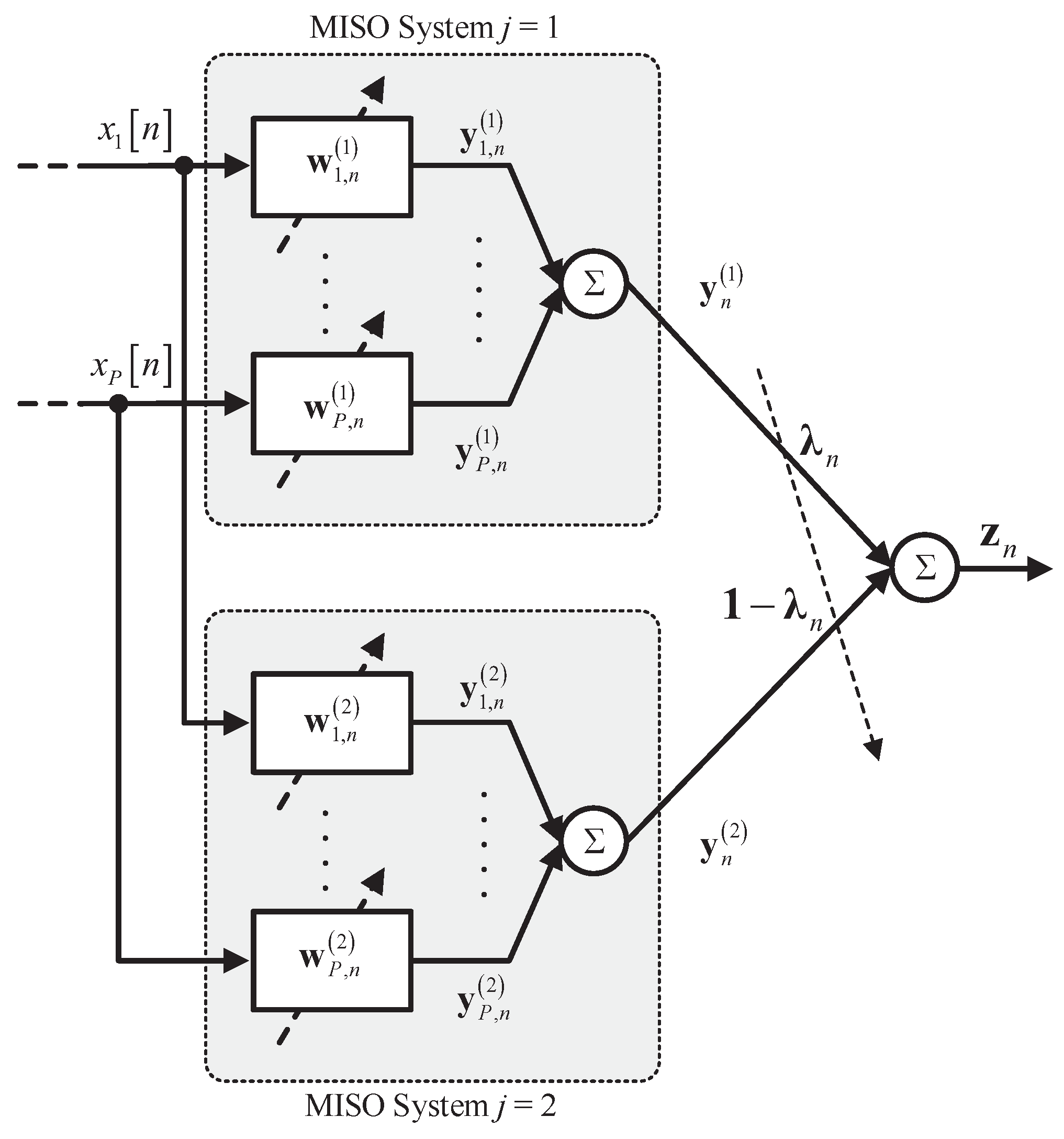
2. A Convex Combination Scheme for Adaptive MISO Filters

An adaptive MISO system is composed of a number P of adaptive filters in parallel, each one receiving a different input, and yields a single output. A combined system of MISO filters is characterized by the adaptive combination of the outputs of different MISO filters, which can be differentiated in several ways according to the updating rule or some parameter settings. In this paper, we consider the adaptive combination of a number of J = 2 MISO filters adapted by using the same updating rule, defined by the regularized multichannel APA [25,27], but different projection orders.
The input signals are the same for each MISO system and are collected into data matrices. However, due to the different projection order, each MISO system uses its own sub-matrix. In particular, the p th input sub-matrix of the j th MISO system, for p = 1 , , P and j = 1 , 2 , is represented as X p , n j R K j × M :
X p , n j = x p , n j x p , n 1 j x p , n K j + 1 j T = x p n x p n M + 1 x p n 1 x p n M x p n K j + 1 x p n M K j + 2
where M is the length of the adaptive filters (same for all) and K j denotes the number of previous entries to keep in memory, i.e., the projection order, for the j th MISO system. The concatenation of sub-matrices (1) provides the input data matrix for each MISO system, i.e., X n j R K j × M P = X 1 , n j X 2 , n j X P , n j . Each MISO filter can be represented by w n j R M P × 1 w 1 , n j , T w 2 , n j , T w P , n j , T T , with j = 1 , 2 . The output vector of each MISO filter y n j R K j × 1 = y 0 j n y 1 j n y K j 1 j n T is then obtained as:
y n j = X n j w n 1 j .
Taking into account the vector d n j R K j × 1 = d n d n 1 d n K j + 1 T containing the last K j samples of the desired signal, it is possible to achieve the error signal vector e n j R K j × 1 = e 0 j n e 1 j n e K j 1 j n T for each MISO filter:
e n j = d n j y n j .
It is worth noting that the difference of notation between the k th entry d n k of d n j and the entry y k n of y n j (and the same for e n j ) is due to the fact that d n j is a regression vector collecting the last K j samples of the desired signal, while all the entries of y n j and e n j are computed at each time instant. This means, for example, that the entry of the desired signal for k = 0 at the n 1 time instant has the same value of the entry for k = 1 at the n th time instant, and they both are denoted with d n 1 . On the other hand, all the entries of the output and signal vectors may change at each time instant until convergence; hence, for example, y 0 j n 1 y 1 j n .
Therefore, the update rule of each MISO filter using the regularized multichannel affine projection algorithm [27,28]:
w n j = w n 1 j + μ j X n j , T δ j I + X n j X n j , T 1 e n j
where μ j is the step size and δ j is the regularization factor for the j th MISO filter, which is considered the same for both MISO filters.
The chosen method for combining MISO filters is the system-by-system combination scheme [8], depicted in Figure 1, since it involves the minimum necessary number of free parameters for single-stage combined architectures. According to this scheme, the overall output of the system is achieved by combining convexly the MISO filter outputs (2). This combination involves the sum of buffers with different lengths, which depends on the projection order K j . This problem is addressed by using zero-padding, thus:
z n R K 1 × 1 = λ n y n 1 + 1 λ n y n 2 ; 0 1 , if K 1 K 2 R K 2 × 1 = λ n y n 1 ; 0 2 + 1 λ n y n 2 , if K 1 < K 2
where 0 1 R K 1 K 2 × 1 and 0 2 R K 2 K 1 × 1 are vectors of zeros, 1 R K max × 1 are vectors of ones, where K max = max K 1 , K 2 , and λ n R K max × 1 are mixing parameter vectors for j = 1 , 2 ; finally, ⊙ denotes the Hadamard product.
The mixing parameters are adaptive weights that balance the combination between the two MISO filters, giving more importance to the best-performing one. Such awareness is obtained according to a mean squared error minimization. The adaptation of λ n is performed by using an auxiliary vector a n , whose elements are related to those of λ n by means of a sigmoidal function defined according to [8,44]:
λ k n = β 1 1 + e a k n 1 α , k = 0 , , K max 1
where:
α = 1 1 + e 4 , β = 1 1 2 α .
The auxiliary vectors are updated by using a gradient descent rule; therefore, for k = 0 , , K max 1 :
a k n = a k n 1 + μ c β r k n e k n y k 1 n y k 2 n · λ k n + α β β α β λ k n
where μ c / r k n represents a normalized step size [45],
r k n = γ r k n 1 + 1 γ y k 1 n y k 2 n 2
is the estimated power of y k 1 n y k 2 n , and γ is a smoothing factor close to one.
The entries e k n in (8), for k = 0 , , K max 1 , of the overall error signal vector e n are derived as:
e n R K max × 1 = d n 1 z n , if K max = K 1 d n 2 z n , if K max = K 2 .
The overall error e n represents the quantity that provides the awareness to the scheme about the best-performing filter, and it is used to adapt the mixing parameters at each iteration, as is possible to note in (8).
The combination described by (5) has a significant value due to its generalization properties, since it can be used:
  • to find an optimal selection of filter parameters, e.g., by choosing different values for the step sizes μ j or for the regularization factors δ j in (4) [1,6];
  • to improve the overall tracking abilities beyond the capabilities of the individual filters by selecting K 1 = 1 and K 2 > 1 . Since the APA with unitary projection order is equivalent to the (normalized) least mean squares algorithm, this choice enables the scheme to show a combination between a gradient-based and a Hessian-based adaptive algorithm, which provides diversity to the scheme and leads to enhancing the tracking performance [1,16].
In those applications having limited computational resources, the complexity of the proposed method may represent a drawback. While the adaptation of the mixing parameters does not involve a significant increment of the computational load [1], the adaption of two MISO filters in parallel may require twice the resources. However, several implementation strategies have been proposed in the literature to reduce the overall complexity of a combined scheme significantly, such as using a low-cost filter as a companion to a high-cost one, rather than using parallelization, or taking advantage of redundancies in the two filter components (see [1] for further details). The implementation of such strategies would make the computational load of the combined scheme just slightly higher than the complexity of a single MISO filter.
In the next sections, we provide a theoretical derivation of the steady-state performance, which is useful to understand the capabilities of the proposed combined filtering scheme.

3. Optimum Mixing Parameters and EMSE

A first step to perform a mean squared performance analysis of the proposed combined scheme consists of deriving the expression of the optimal mixing parameter for each input projection that minimizes the mean squared error of the combined scheme. To this end, we first define the problem formulation, and then, we formalize the combination performance.

3.1. Stationary Data Model

Let us consider the following linear regression model:
d n = x n T w o + v n
where x n R M P × 1 = x 1 , n T x P , n T T is the first projection (i.e., for k = 0 ) of the data input matrix X n j (for the simplicity of notation, we omit the projection order subscript for k = 0 ), and it is the same for both MISO filters. Moreover, in (11), w o R M P × 1 = w 1 o , T w P o , T T is the optimal multichannel weight solution. With respect to the model of (11), we consider the following assumptions [6,41,42].
Assumption 1.
The signal v n represents an independent and identically distributed (i.i.d.) noise added to the system output, whose variance is σ v 2 .
Assumption 2.
The input signals are assumed to be statistically independent of the noise signal.
Assumption 3.
We also assume that E x p , n = 0 , E d n = 0 , E v n = 0 , and define the covariance matrix E x p , n x p , n T = R p , n .
We can define the weight error vector for the j th MISO filter and for the multichannel combined scheme, respectively, as:
w ˜ n j R M P × 1 = w o w n j
w ˜ n R M P × 1 = w o w n
We also introduce the a priori and the a posteriori estimation error signals for the j th MISO system, respectively, as:
e a n j R K j × 1 = e n j v n j = X n j w ˜ n 1 j
e p n j R K j × 1 = X n j w ˜ n j
and the a priori and the a posteriori estimation error signals for the combination scheme, respectively, as:
e a n R K max × 1 = e n v n = X n w ˜ n 1
e p n R K max × 1 = X n w ˜ n
where v n j R K j × 1 = v n v n 1 v n K j + 1 T contains the last K j samples of the irreducible noise, while v n R K max × 1 contains the last K max samples of v n , and x n R K max × 1 .
It is worth noting that while in the steady-state definition of the model (11), we consider the input at its current time instant, in (14) and (16), we take into account also the projections of the input signal.
Considering (10) and (5), the a priori error (16) can be also written as:
e a n R K max × 1 = λ n e a n 1 + 1 λ n e a n 2 ; 0 1 , if K max = K 1 λ n e a n 1 ; 0 2 + 1 λ n e a n 2 , if K max = K 2
which can be denoted for simplicity of notation as:
e a n = λ n e a n 1 + 1 λ n e a n 2

3.2. Formulation of the EMSE for the Combination

The mean squared performance of the combined MISO filter can be evaluated in terms of the excess mean squared error (EMSE) (see for example [1,22,41]), which can be defined according to the expression of the a priori error (19), for k = 0 , , K max 1 :
ξ k n = E e a k n 2 = λ k 2 n E e a k 1 n 2 + 1 λ k n 2 E e a k 2 n 2 + 2 λ k n 1 λ k n E e a k 1 n e a k 2 n = λ k 2 n ξ k 1 n + 1 λ k n 2 ξ k 2 n + 2 λ k n 1 λ k n ξ k 12 n
where ξ k j n , j = 1 , 2 , are the EMSEs of the k th projection for the two individual MISO filters and:
ξ k 12 n = E e a k 1 n e a k 2 n
represents the cross-EMSE, as defined in [6], which provides a measure of the ability of the combination to improve the performance with respect to both filter components [1]. The cross-EMSE satisfies the Cauchy–Schwartz inequality:
ξ k 12 n 2 ξ k 1 n ξ k 2 n
which implies that the magnitude of the cross-EMSE ξ k 12 n can never be simultaneously larger than the individual EMSEs ξ k 1 n and ξ k 2 n .
We want to minimize (20) to find the optimum mixing parameter for each projection. The minimization must take into account that λ k n is contained in the interval 0 , 1 and that (20) is nonnegative and quadratic in λ k n [1]. Therefore, the optimum mixing parameter is given by:
λ k o n = ξ k 2 n ξ k 1 n ξ k 1 n + ξ k 2 n 2 ξ k 12 n 0 1 = Δ ξ k 2 n Δ ξ k 1 n + Δ ξ k 2 n 0 1
where Δ ξ k j n = ξ k j n ξ k 12 n , j = 1 , 2 , and the vertical line denotes the limits of the interval for the optimum mixing parameters.
We now substitute (23) in (20) to find the definition of the optimum EMSE for all the input projections:
ξ k o n = ξ k 1 n 1 λ k o n Δ ξ k 1 n ξ k 2 n λ k o n Δ ξ k 2 n .
The expressions of the optimum EMSE are valid for any time instant n and also at steady state, i.e., for n . It is worth noting from (23) and (24) that the combination depends on the value of the cross-EMSE. In particular, we can identify four different cases [1,6]:
Case 1:
ξ k 1 n ξ k 12 n < ξ k 2 n .
For this case, it is easy to verify that Δ ξ k 1 n 0 and Δ ξ k 2 n > 0 . In this situation, the optimum mixing parameter is λ k o n = 1 , and the combined scheme turns out to perform like the best individual filter, i.e., the one with the lower EMSE, which is the first filter. Indeed, if we replace λ k o n in (24), we achieve:
ξ k o n ξ k 1 n .
Case 2:
ξ k 1 n > ξ k 12 n ξ k 2 n .
Here, we have that Δ ξ k 1 n > 0 and Δ ξ k 2 n 0 . Again, the combined filter turns out to perform like the best individual filter, which in this case is the second one. As a matter of fact, the optimum mixing parameter is λ k o n = 0 ; thus, the optimum EMSE is:
ξ k o n ξ k 2 n .
Case 3:
ξ k 12 n < min ξ k j n , j = 1 , 2 .
In this case, considering (24), it is easy to conclude that the cross-EMSE is lower than both individual EMSEs; therefore, Δ ξ k j n > 0 , j = 1 , 2 , while λ k o n 0 , 1 . This result can be justified by the fact that since the correlation between the a priori errors of both individual components is small, their weighted combination provides an estimation error of reduced variance [1]. In this case, the optimum EMSE is still represented by (24).
Case 4:
ξ k 1 n = ξ k 2 n = ξ k 12 n .
For completeness, we consider also this particular case, whose condition is rather rare to find in practice. In this case, we have Δ ξ k j n = 0 , j = 1 , 2 ; thus, the optimum EMSE is:
ξ k o n = ξ k j n = ξ k 12 n .
From these cases, it can be gathered that when the cross-EMSE is comprised between the two individual EMSEs (i.e., Cases 1 and 2), the cross-correlation between the a priori errors of the two filters is high enough so that their combination can perform at most as the best individual filter. However, when the cross-EMSE is lower than the individual EMSEs (i.e., Case 3), a lower excess error is achieved for the combination.
In order to achieve the expressions of the EMSEs resulting from the above cases, we need to derive the individual EMSEs of the two MISO filters and the cross-EMSE. To this end, we analyze the mean squared performance of the individual MISO filters in Section 4, from which we derive the expressions of ξ k j n = 0 , j = 1 , 2 , and the mean squared performance of the combination in Section 5, from which we derive the cross-EMSE ξ k 12 n .

4. Mean Squared Performance of Individual MISO APA Filters

Individual EMSEs ξ k j n , for j = 1 , 2 and k = 0 , , K max , can be derived by a straightforward extension of the analysis in [42] to the multichannel case. To this end, we derive the energy conservation arguments.

4.1. Energy Conservation Relation for MISO Filters

We can reformulate the update equation of the j th MISO filter (4), j = 1 , 2 , in terms of the weight error vector (12):
w ˜ n j = w ˜ n 1 j μ j X n j , T δ j I + X n j X n j , T 1 e n j .
We left-multiply both sides of (25) by X n j :
X n j w ˜ n j = X n j w ˜ n 1 j μ j X n j X n j , T δ j I + X n j X n j , T 1 e n j
in which we replace the expressions of the a priori and a posteriori estimation errors, respectively (14) and (15), thus yielding:
e p n j = e a n j μ j X n j X n j , T δ j I + X n j X n j , T 1 e n j .
Assuming that X n j X n j , T is invertible, we can rewrite (27) as:
δ j I + X n j X n j , T 1 e n j = 1 μ j X n j X n j , T 1 e a n j e p n j .
Replacing (28) in (25) and rearranging appropriately, we obtain:
w ˜ n j + X n j , T X n j X n j , T 1 e a n j = w ˜ n 1 j + X n j , T X n j X n j , T 1 e p n j .
We evaluate the energy of (29), thus obtaining the energy conservation relation for the j th MISO filter:
w ˜ n j 2 + e a n j , T X n j X n j , T 1 e a n j = w ˜ n 1 j 2 + e p n j , T X n j X n j , T 1 e p n j
in which no approximations are used, but it is an exact relation showing how the energies of the weight-error vectors at two successive iterations are related to the weighted energies of the a priori and a posteriori estimation error vectors [42].

4.2. Variance Relation for MISO Filters

Now, we analyze the energy conservation relation (30) in the mean squared sense. To this end, we take the expectations of both sides of (30) and get:
E w ˜ n j 2 + E e a n j , T X n j X n j , T 1 e a n j = E w ˜ n 1 j 2 + E e p n j , T X n j X n j , T 1 e p n j
Considering that at steady state (i.e., for n ), the weights no longer change, we have that E w ˜ n j 2 = E w ˜ n 1 j 2 , so (31) reduces to:
E e a n j , T X n j X n j , T 1 e a n j = E e p n j , T X n j X n j , T 1 e p n j .
Using (27), the right-hand side of (32) becomes:
μ j E e p n j , T X n j X n j , T 1 e p n j = E e a n j , T X n j X n j , T 1 e a n j μ j E e a n j , T B n j e n j μ j E e n j , T B n j e a n j + μ j 2 E e n j , T A n j e n j
where:
B n j = δ j I + X n j X n j , T 1
A n j = B n j X n j X n j , T B n j .
Replacing (33) in (32), we obtain the variance relation for the j th MISO filter:
μ j E e n j , T A n j e n j = E e a n j , T B n j e n j + E e n j , T B n j e a n j .

4.3. Steady-State Performance for MISO Filters

We want to derive the expressions of individual EMSE at steady state so, taking into account the definition of the a priori estimation error signal for the j th MISO filter (14) and Assumption 2, and neglecting the dependency of w ˜ n 1 j on past noise samples, we can approximate the variance relation (36) as:
μ j E e a n j , T A n j e a n j + μ j E v n j , T A n j v n j = 2 E e a n j , T B n j e a n j .
We use this expression to evaluate the EMSE for n . However, for this purpose, we need a further assumption [42].
Assumption 4.
At steady state, the input signal x n is statistically independent of the a priori estimation error signals e a n j , j = 1 , 2 , and moreover,
E e a n j e a n j , T = E e a j n 2 · S j
where e a j n is the a priori estimation error sample for the first projection (i.e., k = 0 ; we omit the projection order subscript for the simplicity of notation), and the matrix S j R K j × K j assumes the following values:
S j I , for small values of μ j F , for large values of μ j
being F R K j × K j = diag 1 0 0 .
The derivation of the approximation in Assumption 4 can be found in Appendix A.
Using Assumption 4, we can rewrite (37). In particular, the first term on the left-hand side is equivalently written as:
E e a n j , T A n j e a n j = μ j Tr E e a n j e a n j , T A n j = μ j E e a j n 2 Tr S j E A n j .
Similarly, we can write the remaining terms of (37) respectively as follows:
μ j E v n j , T A n j v n j = μ j σ v 2 Tr E A n j
2 E e a n j , T B n j e a n j = 2 E e a j n 2 Tr S j E B n j .
Therefore, (37) becomes:
2 Tr S j E B n j μ j Tr S j E A n j E e a j n 2 = μ j σ v 2 Tr E A n j
from which we can derive the expression of the steady-state EMSE of the individual MISO filters as:
ξ j = lim n E e a j n 2 = μ j σ v 2 Tr E A n j 2 Tr S j E B n j μ j Tr S j E A n j .
It is worth noting that Equation (44) takes into account the information related to each projection and contained in the matrices A n j , B n j and S j , but at the same time, it provides a unique steady-state EMSE value for all the projections; therefore, the dependence of ξ j on index k disappears.
The expression above can be simplified when the regularization factor δ j is small enough, so that A n j B n j . This implies Tr S j E A n j Tr S j E B n j ; hence, the EMSE (44) reduces to:
ξ j = μ j σ v 2 2 μ j Tr E A n j Tr S j E A n j .
Now, we can distinguish two further approximations.
(i)
Small value of μ j .
If we assume a small value of the step size μ j , we have for Assumption 4 that S j = I ; hence, (45) becomes:
ξ j = μ j σ v 2 2 μ j .
(ii)
Large value of μ j .
If we assume a large value of the step size μ j (i.e., close to one), we have for Assumption 4 that S j = F ; hence, (45) becomes:
ξ j = μ j σ v 2 2 μ j Tr E A n j E a 11 j n
where a 11 j n is the element on the first row and first column of A n j . However, we can also assume the following approximations:
Tr E A n j E K j x n 2
1 E a 11 j n Tr R n j
that yield the following expression for the steady-state EMSE of the j th MISO filter:
ξ j = μ j σ v 2 2 μ j Tr R n j E K j x n 2
which depends proportionally on the value of the projection order K j .

5. Mean Squared Performance of the Combination of MISO Filters

Now, we want to derive the expression of the cross-EMSE ξ k 12 n by carrying out similar procedural steps of the previous section, but considering the cross-information, as explained in detail in the following.
In order to derive the energy conservation relation for the combined scheme, similarly to [6], we consider (29) with X n R K max × 1 and multiply the transpose of (29) for j = 1 by (29) itself for j = 2 , and get:
w ˜ n 1 , T w ˜ n 2 + e a n 1 , T X n X n T 1 e a n 2 = w ˜ n 1 1 , T w ˜ n 1 2 + e p n 1 , T X n X n T 1 e p n 2 .
Taking the expectations of both sides of (51) and considering that at steady state E w ˜ n 1 , T w ˜ n 2 = E w ˜ n 1 1 , T w ˜ n 1 2 , we obtain:
E e a n 1 , T X n X n T 1 e a n 2 = E e p n 1 , T X n X n T 1 e p n 2 .
Replacing (27) (with X n R K max × 1 ) in (52) and after some simplifications, similarly to what was done for (36), it is possible to achieve the variance relation for the combined scheme at steady state:
μ 1 μ 2 E e n 1 , T A n e n 2 = μ 1 E e n 1 , T B n e a n 2 + μ 2 E e a n 1 , T B n e n 2
where A n and B n are defined similarly to (34) and (35), respectively, but over K max . Considering (14), we can rewrite (53), similarly to (37), as:
μ 1 μ 2 E e a n 1 , T A n e a n 2 + μ 1 μ 2 E v n T A n v n = μ 1 + μ 2 E e a n 1 , T B n e a n 2 .
Now, similarly to Assumption 4, but with extension to the case of combined MISO filters, we can define the following assumption.
Assumption 5.
At steady state, the input signal x n is statistically independent of the a priori estimation error signals e a n j , j = 1 , 2 , and moreover,
E e a n 1 e a n 2 , T = E e a 1 n e a 2 n · S 12
where the value of S 12 R K max × K max is defined according to the following cases.
  • If we characterize the combination scheme according to the step-size values, generally μ 1 small and μ 2 large, e.g., to find an optimal selection of filter parameters, we have that:
    S 12 F
    where F is defined similarly to (39).
  • On the other hand, if we want to provide diversity to the combined scheme and choose different projection orders, but the same step-size value, i.e., μ 1 = μ 2 = μ , we have that:
    S 12 I , for small values of μ F , for large values of μ .
    Equation (57) holds as long as the SNR is high, as detailed in Appendix B.
The derivation of the approximation (55) in Assumption 5 can be found in Appendix B.
Using Assumption 5 and after some manipulations, similarly to what was done for (44), it is possible to derive the expression of the cross-EMSE from (54):
ξ 12 = lim n E e a 1 n e a 2 n = μ 1 μ 2 σ v 2 Tr E A n μ 1 + μ 2 Tr S 12 E B n μ 1 μ 2 Tr S 12 E A n .
As done in the previous section for ξ j , we may further simplify also (58) when the regularization factor δ j is small enough to be neglected, so that A n B n , which implies:
ξ 12 = μ 12 σ v 2 Tr E A n 1 μ 12 Tr S 12 E A n
where μ 12 = μ 1 μ 2 / μ 1 + μ 2 . Equation (59) can be further reduced according to the values of the step sizes. In particular, similarly to what was done for ξ j in Section 4.3, we can consider the following approximations.
(i)
Small values for both μ j .
This case is typical when we want to differentiate the combined scheme according to the projection order and we choose the same small value for both step sizes μ 1 = μ 2 = μ . Based on Assumption 5, we have that S 12 = I ; hence, (59) becomes:
ξ 12 = μ 12 σ v 2 1 μ 12 .
(ii)
Large value for at least one μ j .
We can also consider the case for which S j = F , according to Assumption 5. This may occur when we want to characterize the combined scheme according to the projection order and we choose the same large value for both step sizes μ 1 = μ 2 = μ , or also when we choose the same projection order, but one step-size value small and the other one large (close to one). In both of these situations, after some approximations similarly to (50), we have that (59) becomes:
ξ 12 = μ 12 σ v 2 1 μ 12 Tr R n E K max x n 2
which depends proportionally on the value of the maximum projection order K max between the two MISO filters.
We can note that, similarly to the case of the individual EMSEs in (44), even the steady-state cross-EMSE (58) provides a unique value for all the projections, although it considers the information related to them. This also implies a unique value at steady state for the optimum mixing parameter for all the projections. Therefore, considering (44) and (58), and related approximations, the expression of the theoretical EMSE of the combined MISO scheme (24) can be written at steady state as:
ξ = ξ 1 n 1 λ Δ ξ 1 ξ 2 λ Δ ξ 2
according to which the four different cases described in Section 3 can be easily derived.

6. Simulation Results

We evaluate the theoretical results derived in the previous sections by considering a system identification scenario. The unknown MISO system, described by the model of (11), was composed of P = 5 impulse responses, each one formed with M = 7 independent random values between 1 and one. The input signal was generated by means of a first-order autoregressive model, whose transfer function is 1 α 2 / 1 α z 1 , with α = 0.8 , fed with an i.i.d. Gaussian random process. The length of the input signal was L = 20,000 samples. An additive i.i.d. noise signal v n with variance σ v 2 = 0.01 (i.e., providing 20 dB of SNR) was added to form the desired signal. We took into account a combined MISO filter to identify the unknown MISO system. We might differentiate the two individual MISO filters of the combined scheme according to the step-size values or to the projection orders.
The theoretical EMSEs were achieved by considering (24), involving (45) and related approximations for individual EMSEs and (59) and related approximations for the cross-EMSE. The measured steady-state EMSEs were achieved according to:
EMSE n = E e n v n 2
evaluated over 50 independent runs. We also report the measured EMSEs of the two individual MISO filters.

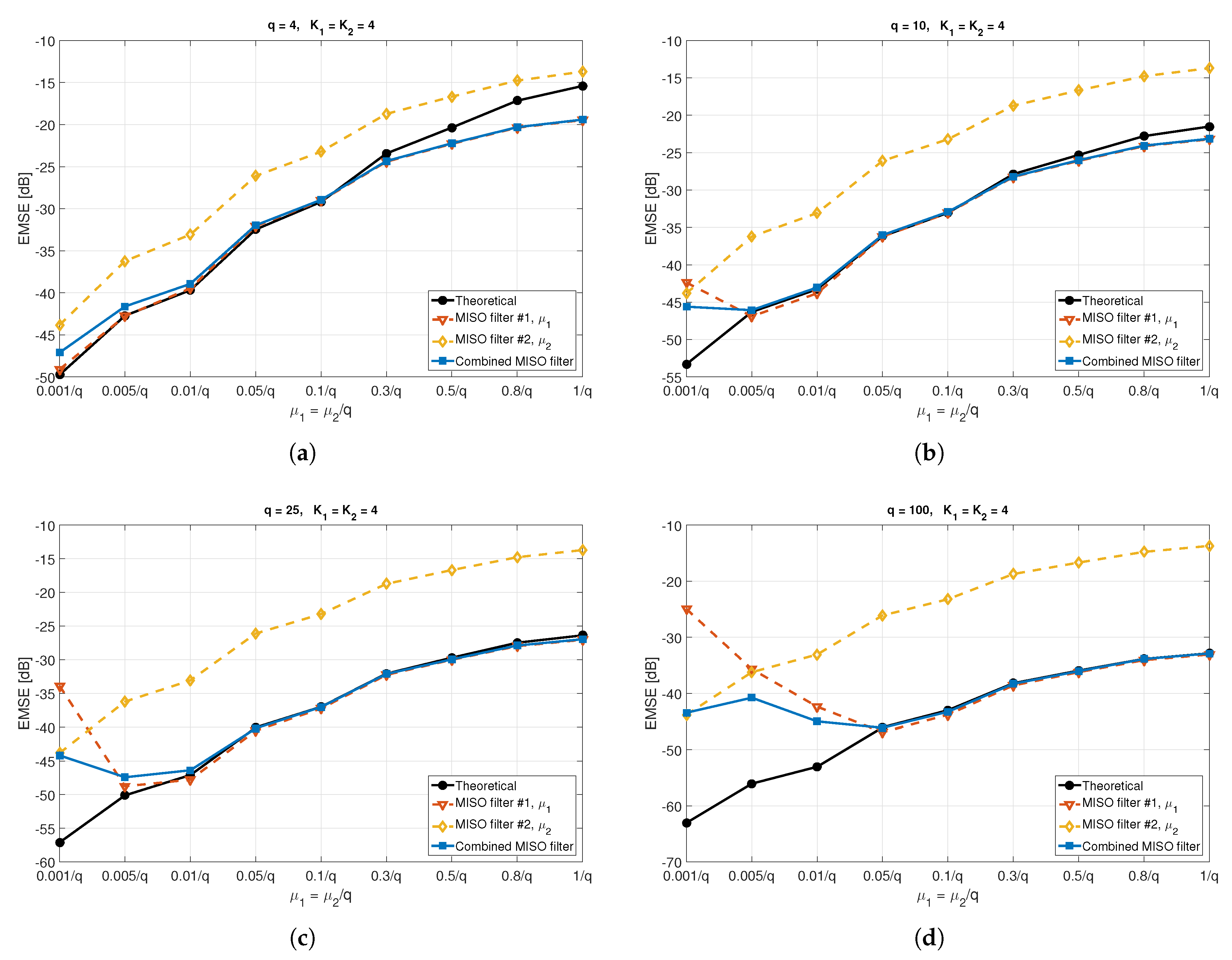
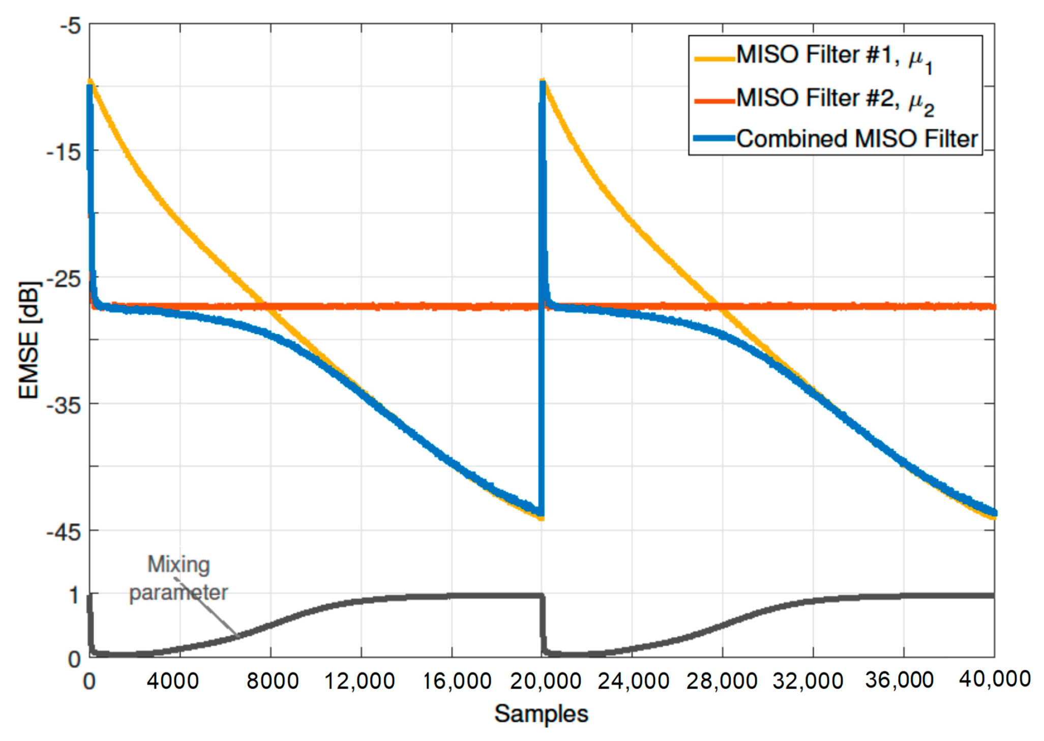
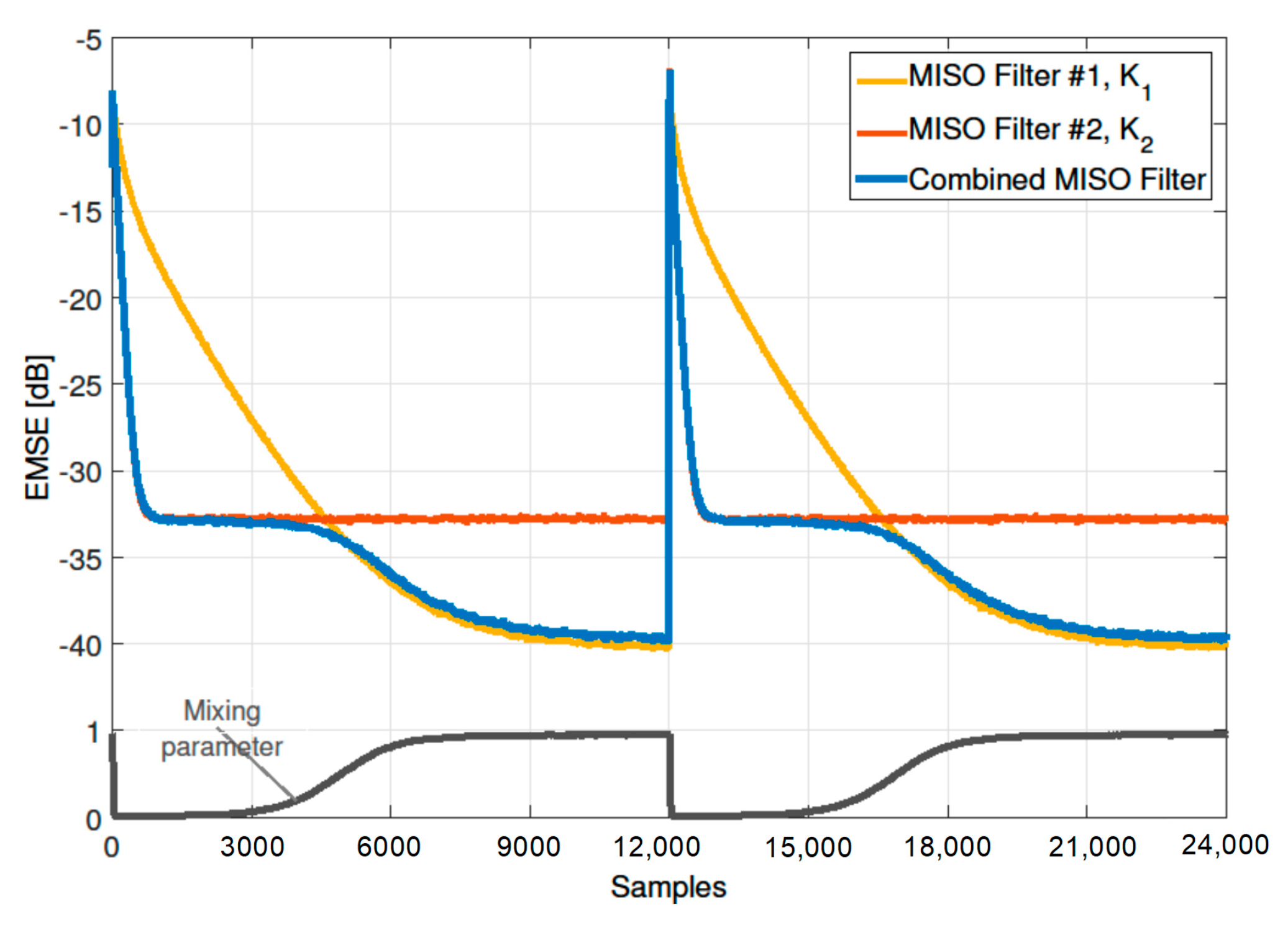
6.1. Performance Evaluation Using Different Step-Size Values

First, we analyzed the former case by choosing different step-size values for the two MISO filters. We chose the same projection order K 1 = K 2 = 4 for both the MISO filters, and we varied the step-size values. In particular, we took into account the range of values 0.001 , 1 for μ 2 , which represents the larger step size, and we set μ 1 = μ 2 / q , where q is a proportionality factor. The parameter setting for the adaptive combination was characterized by: μ c = 0.5 , a k 0 = 0 and r k 0 = 1 for k = 0 , , K max 1 .
The results are shown in Figure 2 with different settings of the factor q, i.e., 4, 10, 25, and 100. These results prove the validity of the derived theoretical EMSE (59), as the measured EMSE values approached the theoretical ones. It is worth noting, in Figure 2, the effect of the combination, especially for small step-size values and high q.
We also evaluated the convergence performance of the combined MISO scheme. The scenario was similar to the previous experiment, but in this case, we considered P = 8 unknown channels, each one formed by M = 10 independent random values between 1 and one. The input signal was again generated by using a first-order autoregressive model, and its length was L = 40,000. In order to study the ability of the combined filtering scheme to react to abrupt changes in the scenario, the coefficients of all the unknown channels were randomly reassigned at time instant n = L / 2 . Again, we considered additive noise with σ v 2 = 0.01 at the output of the unknown MISO system. We chose a small step-size value μ 1 = 0.001 for the first MISO filter and a larger one μ 2 = 0.1 for the second MISO filter, while we considered the same projection order K 1 = K 2 = 2 for both filters. Performance was evaluated in terms of the measured EMSE, averaged over 10,000 independent runs. We compared the adaptive combined MISO filter with the corresponding individual filters. Results are depicted in Figure 3, where it is worth noting that the MISO filter with μ 1 shows a slow convergence rate, but a good precision at steady state, while the MISO filter with μ 2 provides a faster convergence rate, but lower precision. The combined MISO filter was capable of exploiting the advantages of both the individual MISO filters, thus showing a fast convergence rate and good precision at steady state. Moreover, a performance gain due to the cross-EMSE was visible when the mixing parameter was changing its value from zero to one. In Figure 3, the evolution of the current projection of the mixing parameter, i.e., for k = 0 , is also depicted to highlight the changing behavior of the combined MISO filter.

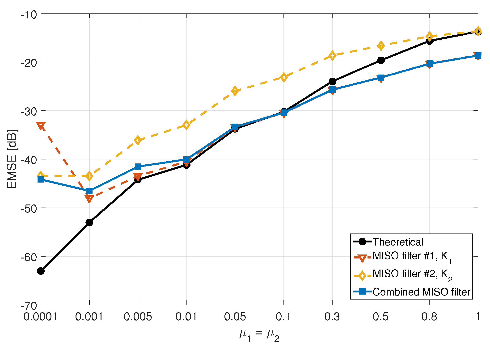
6.2. Performance Evaluation Using Different Projection Orders

We analyzed also the second case of combination by differentiating the MISO filters according to the projection orders, which is very important since the combination of APA-based filters with different projection orders is able to provide diversity to the combined scheme [1,16]. In particular, we chose K 1 = 1 for the first MISO filter, which turns out to be a multichannel NLMSfilter, and K 2 = 4 for the second MISO filter. The parameter setting for the adaptive combination was the same as used for the first case. Different selections have been chosen for the step-size value, which was the same for both the individual MISO filters. We compared the theoretical values of the EMSE of (59) for the combined architecture with the measured steady-state EMSEs of (63) over 50 independent runs. We also compared the measured EMSEs of the two individual MISO filters. Results are shown in Figure 4 and prove the validity of (59), as again, the measured EMSE values approached the theoretical ones.
Even for this case, we evaluated the convergence performance of the combined MISO scheme. The scenario was the same as in the first case, and the input signal length was L = 24,000. Again, we considered an abrupt change at time instant n = L / 2 . The combined MISO filter was composed of two individual MISO filters having different projection orders, K 1 = 1 and K 2 = 4 , and same step sizes, μ 1 = μ 2 = 0.01 . Performance was evaluated in terms of the measured EMSE (63), averaged over 10,000 independent runs. We compared the adaptive combined MISO filter with the corresponding individual filters. The results are depicted in Figure 5, where it is possible to notice that even in this case, the combined MISO filter was capable of exploiting the advantages of both the individual MISO filters, as also highlighted by the evolution of the mixing parameter on the current projection (i.e., λ 0 n ).

7. Conclusions

In this paper, we have studied an adaptive combination of MISO filters, based on the adaptation by the multichannel APA, which allows the filters to be differentiated according to the step size or to the projection order. We have analyzed the steady-state performance of such a combined scheme, thus deriving a theoretical value for the EMSE based on the energy conservation properties. Simulation results have proven the validity of such a theoretical study. We have also assessed the performance improvement involved by an adaptive combined MISO filter using different projection orders in a changing scenario. Future research lines include the analysis of tracking and the transient performance of a combined MISO filter, as well as the extension to multi-stage combined filtering architectures. Moreover, the scheme can be evaluated in practical system identification problems, like acoustics or communications applications, where its performance can be compared with that of alternative single-MISO adaptive filters, such as multichannel variable step-size APA filters.

Author Contributions

Conceptualization, D.C.; formal analysis, D.C.; investigation, D.C., M.S., and L.A.A.-R.; methodology, D.C.; software, D.C.; supervision, A.U.; validation, D.C.; writing, original draft, D.C.; writing, review and editing, D.C., M.S., and L.A.A.-R.

Funding

The work of Danilo Comminiello, Michele Scarpiniti and Aurelio Uncini has been supported by the project: “Vehicular Fog energy-efficient QoS mining and dissemination of multimedia Big Data streams (V-FoG and V-Fog2)”, funded by Sapienza University of Rome Bando 2016 and 2017. The work of Michele Scarpiniti and Aurelio Uncini has been also supported by the project: “GAUChO – A Green Adaptive Fog Computing and networking Architectures” funded by the MIUR Progetti di Ricerca di Rilevante Interesse Nazionale (PRIN) Bando 2015, grant 2015YPXH4W_004. The work of Luis A. Azpicueta-Ruiz is partially supported by the Spanish Ministry of Economy and Competitiveness (under grant DAMA (TIN2015-70308-REDT) and grants TEC2014-52289-R and TEC2017-83838-R), and by the European Union.

Conflicts of Interest

The authors declare no conflict of interest.

Appendix A. Steady-State Approximation for the EMSE of Individual MISO Filters with Multiple Projections

We evaluate the term E e a n j e a n j , T . We remind the reader that the vectors e a n j R K j × 1 and e p n j R K j × 1 , with j = 1 , 2 , contain the projections of the a priori and a posteriori estimation errors, respectively, at the n th time instant, and they can be written as:
e a n j = e a 0 j n e a K max 1 j n T
e p n j = e p 0 j n e p K max 1 j n T .
Assuming a small value for the regularization parameter δ j , the relation between the a priori and the a posteriori estimation error signals in (27) becomes:
e p n j = e a n j μ j e n j = 1 μ j e a n j μ j v n j .
Taking the expectation of the square of both sides of (A3) and considering the error signals to be statistically independent of the noise, we have:
E e p n j e p n j , T = 1 μ j 2 E e a n j e a n j , T + μ j 2 σ v 2 .
At steady state, we know that the coefficients of the weight vectors no longer change [41]. We also know that, due to the construction of the input data matrix, in the APA, the k 1 th projection of the input signal at the n th time instant is equivalent to the k th projection at the time instant n 1 [41,42]. Therefore, at steady state, the k 1 projection of the a posteriori error is equivalent to the k th projection of the a priori error signal. For this reason, the expectation in (A4) can be rewritten, for k = 1 , , K j 1 , as:
E e a k j n 2 = 1 μ j 2 E e a k 1 j n 2 + μ j 2 σ v 2
while for k = 0 , E e a 0 j n 2 is initialized to its own value, which we write omitting the index k = 0 .
Generalizing (A5) for all the projections, we have:
E e a n j e a n j , T = E e a j n 2 · S j + μ j 2 σ v 2 · S v j
where S j and S v j are diagonal matrices R K j × K j , respectively given by:
S j = diag 1 ζ ζ 2 ζ K j 1
S v j = diag 0 1 ζ + 1 ζ 2 + ζ + 1 ζ K j 2 + ζ K j 3 + + 1
where ζ = 1 μ j 2 .
It is worth noting that, when μ j is small, S j I . On the other hand, when μ j is close to one, S j F , where F = diag 1 0 0 . Regarding the second term of the right-hand side of (A6), μ j 2 σ v 2 S v j 0 , when μ j is small enough or when the SNR (signal-to-noise ratio) is high enough (i.e., σ v 2 very small).
In addition, considering that the choice of large values of μ j might not lead to satisfactory convergence performance when the SNR is low, we can always neglect the term μ j 2 σ v 2 S v j in (A6). Therefore, steady-state EMSE for the j th MISO filter evaluated at all the projections can be finally written as:
E e a n j e a n j , T = E e a j n 2 · S j = ξ j S j .

Appendix B. Steady-State Approximation for the Cross-EMSE Involving Multiple Projections

Assuming a small value for the regularization parameter δ and considering the relation between the a priori and the a posteriori estimation error signals in (A3), we take the expectation E e a n 1 e a n 2 , T and get:
E e p n 1 e p n 2 , T = 1 μ 1 1 μ 2 E e a n 1 e a n 2 , T + μ 1 μ 2 σ v 2 .
Similarly to Appendix A, we can rewrite (A10) as:
E e a n 1 e a n 2 , T = E e a 1 n e a 2 n · S 12 + μ 1 μ 2 σ v 2 · S v 12
where S 12 and S v 12 are diagonal matrices R K max × K max , respectively given by:
S 12 = diag 1 ζ c ζ c 2 ζ c K max 1
S v 12 = diag 0 1 ζ c + 1 ζ c 2 + ζ c + 1 ζ c K max 2 + ζ c K max 3 + + 1
where ζ c = 1 μ 1 1 μ 2 .
It is worth noting that, when both μ 1 and μ 2 are small, S 12 I . On the other hand, when at least one of the step-size values is close to one, S 12 F .
Concerning the second term of the right-hand side of (A11), μ 1 μ 2 σ v 2 S v 12 0 when at least one of the step sizes is small enough or when the noise power is low (i.e., σ v 2 very small). In addition, considering that for low SNR values, the choice of large values for both the step sizes might not lead to satisfactory convergence performance, we can always neglect the term μ 1 μ 2 σ v 2 S v 12 in (A11). Therefore, (A11) can be written as:
E e a n 1 e a n 2 , T = E e a 1 n e a 2 n · S 12 = ξ 12 S 12 .

References

  1. Arenas-García, J.; Azpicueta-Ruiz, L.A.; Silva, M.T.M.; Nascimento, V.H.; Sayed, A.H. Combinations of Adaptive Filters: Performance and Convergence Properties. IEEE Signal Process. Mag. 2016, 1, 120–140. [Google Scholar] [CrossRef]
  2. Singer, A.C.; Feder, M. Universal Linear Prediction by Model Order Weighting. IEEE Trans. Signal Process. 1999, 47, 2685–2699. [Google Scholar] [CrossRef]
  3. Kozat, S.S.; Singer, A.C. Multi-Stage Adaptive Signal Processing Algorithms. In Proceedings of the IEEE Sensor Array Multichannel Signal Workshop (SAM), Cambridge, MA, USA, 17 March 2000; pp. 380–384. [Google Scholar]
  4. Yousef, N.R.; Sayed, A.H. A Unified Approach to the Steady-State and Tracking Analyzes of Adaptive Filters. IEEE Trans. Signal Process. 2001, 49, 314–324. [Google Scholar] [CrossRef]
  5. Arenas-García, J.; Martínez-Ramón, M.; Navia-Vázquez, A.; Figueiras-Vidal, A.R. Plant Identification via Adaptive Combination of Transversal Filters. Signal Process. 2006, 86, 2430–2438. [Google Scholar] [CrossRef]
  6. Arenas-García, J.; Figueiras-Vidal, A.R.; Sayed, A.H. Mean-Square Performance of a Convex Combination of Two Adaptive Filters. IEEE Trans. Signal Process. 2006, 54, 1078–1090. [Google Scholar] [CrossRef]
  7. Arenas-García, J.; Figueiras-Vidal, A.R. Adaptive Combination of Proportionate Filters for Sparse Echo Cancellation. IEEE Trans. Audio Speech Lang. Process. 2009, 17, 1087–1098. [Google Scholar] [CrossRef]
  8. Comminiello, D.; Scarpiniti, M.; Parisi, R.; Uncini, A. Combined Adaptive Beamforming Schemes for Nonstationary Interfering Noise Reduction. Signal Process. 2013, 93, 3306–3318. [Google Scholar] [CrossRef]
  9. Azpicueta-Ruiz, L.A.; Zeller, M.; Figueiras-Vidal, A.R.; Arenas-García, J.; Kellermann, W. Adaptive Combination of Volterra Kernels and its Application to Nonlinear Acoustic Echo Cancellation. IEEE Trans. Audio Speech Lang. Process. 2011, 19, 97–110. [Google Scholar] [CrossRef]
  10. Comminiello, D.; Scarpiniti, M.; Azpicueta-Ruiz, L.A.; Arenas-García, J.; Uncini, A. Functional Link Adaptive Filters for Nonlinear Acoustic Echo Cancellation. IEEE Trans. Audio Speech Lang. Process. 2013, 21, 1502–1512. [Google Scholar] [CrossRef]
  11. Comminiello, D.; Scardapane, S.; Scarpiniti, M.; Parisi, R.; Uncini, A. Convex Combination of MIMO Filters for Multichannel Acoustic Echo Cancellation. In Proceedings of the IEEE International Symposium on Image and Signal Processing (ISPA), Trieste, Italy, 4–6 September 2013; pp. 771–775. [Google Scholar]
  12. Silva, M.T.M.; Arenas-García, J. A Soft-Switching Blind Equalization Scheme via Convex Combination of Adaptive Filters. IEEE Trans. Signal Process. 2013, 61, 1171–1182. [Google Scholar] [CrossRef]
  13. Comminiello, D.; Scarpiniti, M.; Azpicueta-Ruiz, L.A.; Arenas-García, J.; Uncini, A. A Block-Based Combined Scheme Exploiting Sparsity in Nonlinear Acoustic Echo Cancellation. In Proceedings of the IEEE 26th International Workshop on Machine Learning for Signal Processing (MLSP), Salerno, Italy, 13–16 September 2016; pp. 1–6. [Google Scholar]
  14. Comminiello, D.; Scarpiniti, M.; Azpicueta-Ruiz, L.A.; Arenas-García, J.; Uncini, A. Combined Nonlinear Filtering Architectures Involving Sparse Functional Link Adaptive Filters. Signal Process. 2017, 135, 168–178. [Google Scholar] [CrossRef]
  15. Comminiello, D.; Scarpiniti, M.; Scardapane, S.; Azpicueta-Ruiz, L.A.; Uncini, A. Combined Sparse Regularization for Nonlinear Adaptive Filters. In Proceedings of the 26th European Signal Processing Conference (EUSIPCO), Rome, Italy, 3–7 September 2018; pp. 341–345. [Google Scholar]
  16. Silva, M.T.M.; Nascimento, V.H. Improving the Tracking Capability of Adaptive Filters Via Convex Combination. IEEE Trans. Signal Process. 2008, 56, 3137–3149. [Google Scholar] [CrossRef]
  17. Bershad, N.J.; Bermudez, J.C.M.; Tourneret, J.Y. An Affine Combination of two LMS Adaptive Filters— Transient Mean-Square Analysis. IEEE Trans. Signal Process. 2008, 56, 1853–1864. [Google Scholar] [CrossRef]
  18. Candido, R.; Silva, M.T.M.; Nascimento, V.H. Transient and Steady-State Analysis of the Affine Combination of Two Adaptive Filters. IEEE Trans. Signal Process. 2010, 58, 4064–4078. [Google Scholar] [CrossRef]
  19. Kozat, S.S.; Erdogan, A.T.; Singer, A.C.; Sayed, A.H. Steady-State MSE Perfromance Analysis of Mixture Approaches to Adaptive Filtering. IEEE Trans. Signal Process. 2010, 58, 4050–4063. [Google Scholar] [CrossRef]
  20. Donmez, M.A.; Kozat, S.S. Steady State and Transient MSE Analysis of Convexly Constrained Mixture Methods. IEEE Trans. Signal Process. 2012, 60, 3314–3321. [Google Scholar] [CrossRef]
  21. Li, J.; Stoica, P. (Eds.) Robust Adaptive Beamforming; Wiley: Hoboken, NJ, USA, 2005. [Google Scholar]
  22. Uncini, A. Fundamentals of Adaptive Signal Processing; Springer: Cham, Switzerland, 2015; ISBN 978-3-319-02806-4. [Google Scholar]
  23. Hong, E.; Har, D. Peak-to-Average Power Ratio Reduction for MISO OFDM Systems with Adaptive All-Pass Filters. IEEE Trans. Wirel. Commun. 2011, 10, 3163–3167. [Google Scholar] [CrossRef]
  24. Slock, D.T.M. Spatio-Temporal Training-Sequence Based Channel Equalization and Adaptive Interference Cancellation. In Proceedings of the IEEE International Conference on Acoustics, Speech and Signal Processing (ICASSP), Atlanta, GA, USA, 7–10 May 1996; pp. 2714–2717. [Google Scholar]
  25. Gay, S.L.; Benesty, J. (Eds.) Acoustic Signal Processing for Telecommunications; Kluwer Academic Publishers: Boston, MA, USA; Dordrecht, The Netherlands; London, UK, 2000. [Google Scholar]
  26. Thüne, P.; Enzner, G. Trends in Adaptive MISO System Identification for Multichannel Audio Reproduction and Speech Communication. In Proceedings of the 8th International Symposium on Image and Signal Processing and Analysis (ISPA), Trieste, Italy, 4–6 September 2013; pp. 767–772. [Google Scholar]
  27. Ozeki, K.; Umeda, T. An Adaptive Filtering Algorithm Using an Orthogonal Projection to an Affine Subspace and its Properties. Electron. Commun. Jpn. (Part I Commun.) 1984, 67, 19–27. [Google Scholar] [CrossRef]
  28. Benesty, J.; Duhamel, P.; Grenier, Y. A Multichannel Affine Projection Algorithm with Applications to Multichannel Acoustic Echo Cancellation. IEEE Signal Process. Lett. 1996, 3, 35–37. [Google Scholar] [CrossRef]
  29. Albu, F.; Paleologu, C.; Benesty, J. A Variable Step Size Evolutionary Affine Projection Algorithm. In Proceedings of the IEEE International Conference on Acoustics, Speech and Signal Processing (ICASSP), Prague, Czech Republic, 22–27 May 2011; pp. 429–432. [Google Scholar]
  30. Paleologu, C.; Benesty, J.; Albu, F.; Ciochină, S. An Efficient Variable Step-Size Proportionate Affine Projection Algorithm. In Proceedings of the IEEE International Conference on Acoustics, Speech and Signal Processing (ICASSP), Prague, Czech Republic, 22–27 May 2011; pp. 77–80. [Google Scholar]
  31. Gonzalez, A.; Albu, F.; Ferrer, M.; de Diego, M. Evolutionary and Variable Step Size Strategies for Multichannel Filtered-x Affine Projection Algorithms. IET Signal Process. 2012, 7, 471–476. [Google Scholar] [CrossRef]
  32. Albu, F.; Coltuc, D.; Comminiello, D.; Scarpiniti, M. The Variable Step Size Regularized Block Exact Affine Projection Algorithm. In Proceedings of the 10th International Symposium on Electronics and Telecommunications (ISETC), Timisoara, Romania, 15–16 November 2012; pp. 283–286. [Google Scholar]
  33. Bhotto, M.Z.A.; Ahmad, M.O.; Swamy, M.N.S. Robust Shrinkage Affine-Projection Sign Adaptive-Filtering Algorithms for Impulsive Noise Environments. IEEE Trans. Signal Process. 2014, 62, 3349–3359. [Google Scholar] [CrossRef]
  34. Ferrer, M.; de Diego, M.; Gonzalez, A.; Piñero, G. Convex Combination of Affine Projection Algorithms. In Proceedings of the European Signal Processing Conference (EUSIPCO), Glasgow, UK, 24–28 August 2009; pp. 431–435. [Google Scholar]
  35. Ferrer, M.; de Diego, M.; Gonzalez, A.; Piñero, G. Steady-State Mean Square Performance of the Multichannel Filtered-X Affine Projection Algorithm. IEEE Trans. Signal Process. 2012, 60, 2771–2785. [Google Scholar] [CrossRef] [Green Version]
  36. Arévalo, L.; Apolinário, J.A., Jr.; de Campos, M.L.R.; Sampaio-Neto, R. Convex Combination of Three Affine Projections Adaptive Filters. In Proceedings of the IEEE International Symposium on Wireless Communication Systems (ISWCS), Ilmenau, Germany, 27–30 August 2013; pp. 209–213. [Google Scholar]
  37. Shi, L.; Lin, Y.; Xie, X. Combination of Affine Projection Sign Algorithms for Robust Adaptive Filtering in Non-Gaussian Impulsive Interference. Electron. Lett. 2014, 50, 466–467. [Google Scholar] [CrossRef]
  38. Huang, F.; Zhang, J.; Zhang, S. Combined-Step-Size Affine Projection Sign Algorithm for Robust Adaptive Filtering in Impulsive Interference Environments. IEEE Trans. Circuits Syst. II Express Briefs 2016, 63, 493–497. [Google Scholar] [CrossRef]
  39. Choi, J.H.; Kim, S.H.; Kim, S.W. Adaptive Combination of Affine Projection and NLMS Algorithms. Signal Process. 2014, 100, 64–70. [Google Scholar] [CrossRef]
  40. Comminiello, D.; Scarpiniti, M.; Scardapane, S.; Parisi, R. Improving Nonlinear Modeling Capabilities of Functional Link Adaptive filters. Neural Netw. 2015, 69, 51–59. [Google Scholar] [CrossRef]
  41. Sayed, A.H. Adaptive Filters; Wiley: Hoboken, NJ, USA, 2008. [Google Scholar]
  42. Shin, H.C.; Sayed, A.H. Mean-Square Performance of a Family of Affine Projection Algorithms. IEEE Trans. Signal Process. 2004, 52, 90–102. [Google Scholar] [CrossRef]
  43. Sankaran, S.G.; Beex, A.A.L. Convergence Behavior of Affine Projection Algorithms. IEEE Trans. Signal Process. 2000, 48, 1086–1096. [Google Scholar] [CrossRef]
  44. Lázaro-Gredilla, M.; Azpicueta-Ruiz, L.A.; Figueiras-Vidal, A.R.; Arenas-García, J. Adaptively Biasing the Weights of Adaptive Filters. IEEE Trans. Signal Process. 2010, 58, 3890–3895. [Google Scholar] [CrossRef] [Green Version]
  45. Azpicueta-Ruiz, L.A.; Figueiras-Vidal, A.R.; Arenas-García, J. A Normalized Adaptation Scheme for the Convex Combination of Two Adaptive Filters. In Proceedings of the IEEE International Conference on Acoustics, Speech and Signal Processing (ICASSP), Las Vegas, NV, USA, 31 March–4 April 2008; pp. 3301–3304. [Google Scholar]
Figure 1. System-by-system combination scheme of two adaptive MISO filters.
Algorithms 12 00002 g001
Figure 2. Steady-state theoretical and measured excess mean squared error (EMSE) for a combined MISO filter using different step-size values, according to μ 1 = μ 2 / q , with (a) q = 4 , (b) q = 10 , (c) q = 25 , and (d) q = 100 .
Algorithms 12 00002 g002
Figure 3. Convergence performance of a combined MISO filter using different step-size values with the related evolution of the mixing parameter λ 0 n .
Algorithms 12 00002 g003
Figure 4. Steady-state theoretical and measured EMSE for a combined MISO filter using different projection orders.
Algorithms 12 00002 g004
Figure 5. Convergence performance of a combined MISO filter using different projection orders with the related evolution of the mixing parameter λ 0 n .
Algorithms 12 00002 g005

