Time Series Forecasting Using a Two-Level Multi-Objective Genetic Algorithm: A Case Study of Maintenance Cost Data for Tunnel Fans

Abstract

The aim of this study has been to develop a novel two-level multi-objective genetic algorithm (GA) to optimize time series forecasting data for fans used in road tunnels by the Swedish Transport Administration (Trafikverket). Level 1 is for the process of forecasting time series cost data, while level 2 evaluates the forecasting. Level 1 implements either a multi-objective GA based on the ARIMA model or a multi-objective GA based on the dynamic regression model. Level 2 utilises a multi-objective GA based on different forecasting error rates to identify a proper forecasting. Our method is compared with using the ARIMA model only. The results show the drawbacks of time series forecasting using only the ARIMA model. In addition, the results of the two-level model show the drawbacks of forecasting using a multi-objective GA based on the dynamic regression model. A multi-objective GA based on the ARIMA model produces better forecasting results. In level 2, five forecasting accuracy functions help in selecting the best forecasting. Selecting a proper methodology for forecasting is based on the averages of the forecasted data, the historical data, the actual data and the polynomial trends. The forecasted data can be used for life cycle cost (LCC) analysis.

1. Introduction

Time series forecasting predicts future data points based on observed data over a period known as the lead-time. The purpose of forecasting data points is to provide a basis for economic planning, production planning, production control and optimizing industrial processes. The major objective is to obtain the best forecast function, i.e., to ensure that the mean square of the deviation between the actual and the forecasted values is as small as possible for each lead-time [1,2]. Much effort has been devoted over the past few decades to the development and improvement of time series forecasting models [3].

Traditional models for time series forecasting, such as the Box-Jenkins or autoregressive integrated moving average (ARIMA) model, assume that the studied time series are generated from linear processes. However, these models may be inappropriate if the underlying mechanism is nonlinear. In fact, real-world systems are often nonlinear [4,5]. The multi-objective genetic algorithm (GA) is often compatible with nonlinear systems and uses a particular optimization from the principle of natural selection of the optimal solution on a wide range of forecasting populations [6,7].

The proposed multi-objective GA optimizes a particular function based on the ARIMA model. The ARIMA model is a stochastic process modelling framework [1] that is defined by three parameters $\left(p,d,q\right)$. The parameter $p$ stands for the order of the autoregressive $AR\left(p\right)$ process, $d$ for the order of integration (needed for the transformation into a stationary stochastic process), and $q$ for the order of the moving average process, $MA\left(q\right)$ [8]. A stationary stochastic process means a process where the data properties have the same variance and autocorrelation [9]. The weakness of the ARIMA model is the difficulty of estimating the parameters. To address this problem, a process for automated model selection needs to be implemented in the automated optimization to achieve an accurate forecasting [10].

The GA is a well-established method which helps in solving complex and nonlinear problems that often lead to cases where the search space shows a curvy landscape with numerous local minima. The multi-objective GA is designed to find the best forecasting solution through automated optimization of the ARIMA model and to select the best parameters $\left(p,d,q\right)$ to compute point forecasts based on time series data. The parameters of the ARIMA model are influenced by the selecting process of the GA. In addition, the multi-objective GA can evaluate the forecasting accuracy using multiple fitness functions based on statistics models.

Vantuch and Zelinka [11] modified the ARIMA model based on the genetic algorithm and particle swarm optimization (PSO) to estimate and predict data of time. They found that the genetic algorithm could find a suitable ARIMA model and pointed to improvements through individual binary randomization for every parameter input of the ARIMA model. Their model shows the best set of coefficients obtained with PSO compared with the best set obtained with a classical ARIMA prediction. However, these authors present the ARIMA parameters in a binary setting with limited possibilities and they consider the forecasting based on an ARIMA evaluation only.

Wang & Hsu [12] proposed a combination of grey theory and the genetic algorithm to overcome industrial development constraints and establish a high-precision forecasting model. They used a genetic algorithm to optimize grey forecasting model parameters. They demonstrated a successful application of their model which provided an accurate forecasting with a low forecasting error rate. However, these authors proposed randomization in combination with grey theory without integrating grey theory functionality within the GA. They used only one forecasting error rate to judge the forecasting accuracy.

Ervural et al. [13] proposed a forecasting method based on an integrated genetic algorithm and the ARMA model in order to gain the advantage of both of these tools in the forecasting of data. They used a genetic algorithm to optimize $AR\left(p\right)$ and $MA\left(q\right)$ and find the best ARMA model for the problem. They found that their model had an effective identification for estimating ARMA autoregression and moving averages. However, these authors presented ARIMA parameters with limited possibilities. In addition, they used only one forecasting error rate to judge the forecasting accuracy.

Lin et al. [14] maintained that the back-propagation neural network (BPNN) can easily fall into the local minimum point in time series forecasting. They developed a hybrid approach that combines the adaptive differential evolution (ADE) algorithm with the BPNN. This approach was called the ADE-BPNN and was designed to improve the forecasting accuracy of the BPNN. The initial connection weights and thresholds of the BPNN as a single hidden layer are selected by combining the ADE with the BPNN. The ADE is used to search preliminarily for the global optimal connection weights and thresholds of the BPNN. The ADE is adopted to explore the search space and detect potential regions. The model of Lin et al. [14] shows good performance in solving complex optimization problems. However, their model needs to be improved to handle complex application problems and find the best appropriate structure and parameters.

Yu-Rong et al. [15] utilised the ADE-BPNN to estimate energy consumption. The hybrid model created by these authors incorporates gross domestic product, population, import, and export data as inputs. In this approach, an improved differential evolution with adaptive mutation and crossover is utilised to find appropriate global initial connection weights and thresholds to enhance the forecasting performance of the BPNN. Yu-Rong et al. [15] used an adaptive DE (ADE) algorithm to find appropriate initial connection weights and thresholds of a BPNN for obtaining more accurate forecasting. The BPNN was utilised to achieve good-fitting performance and high forecasting precision. A BPNN is a multilayer mapping network that minimizes errors backward while transmitting information. The prediction accuracy of the authors’ method is relatively high because an improved ADE with good balance between the search speed and accuracy assists in finding appropriate global initial connection weights and thresholds to enhance the forecasting performance of the BPNN effectively. However, their model needs to be improved for long-term forecasts and processing big data.

Lin et al. [16] proposed a combination model resulting from a new neural networks-based linear ensemble framework (NNsLEF). The proposed framework can merge the advantages of component neural networks and dynamic weight combination approaches to improve the forecasting performance. Four neural network models are applied to impart their superior performance to the combination approach while maintaining their diversity. The framework proposed by Lin et al. [16] adheres to three primary principles. (a) Four kinds of neural network models, namely the back-propagation neural network, an artificial neural network with a dynamic architecture, the Elman artificial neural network, and the echo state network, are selected as component forecasting models. (b) An input-hidden selection heuristic (IHSH) is designed to determine the input-hidden neuron combination for each component neural network. (c) An in-sample training-validation pair-based neural network weighting (ITVPNNW) mechanism is studied to generate the associated combination weights. The NNsLEF aims to improve the accuracy of time series forecasting and could provide an effective forecast through the mentioned combination model. However, this approach has limitations and its complexity means that there are a low number of relevant application areas with large data samples.

Hatzakis & Wallace [6] proposed a method that combines the ARIMA forecasting technique and a multi-objective GA based on the Pareto optimal to predict the next optimum. Their method is based on historical optimums and is used to optimize $AR\left(p\right)$ and $MA\left(q\right)$ to find a non-dominated Pareto front solution with an infinite number of points. They found that their method improved the prediction accuracy. However, these authors assumed that the data were accurate and used the Pareto front solution to select a proper forecasting. In addition, they did not use any forecasting error rate to evaluate the forecasting results.

The aim of this study has been to develop a novel two-level multi-objective GA to optimize time series forecasting in order to forecast cost data for fans used in road tunnels. The first level of the GA is responsible for the process of forecasting time series cost data, while the second level evaluates the forecasting. The first level implements either a multi-objective GA based on the ARIMA model or a multi-objective GA based on the dynamic regression model. This level gives possibilities of finding the optimal forecasting solution. The second level utilises a multi-objective GA based on different forecasting error rates to identify a proper forecasting. Our method is compared with the approach of using an ARIMA model only. We argue that a multi-objective GA decreases the complexity, increases the flexibility, and is very effective when selecting an approximate solution interval for forecasting.

The remainder of the paper is organized as follows. The next section presents the materials and methods, which include data collection, the ARIMA model, a two-level multi-objective GA based on the ARIMA model, a two-level multi-objective GA based on the dynamic regression model and a model evaluation method. Section 3 describes the results and decisions for each method presented in the previous section. Section 4 offers the concluding remarks.

2. Materials and Methods

2.1. Data Collection

The cost data concern tunnel fans installed in Stockholm in Sweden. The data had been collected over ten years from 2005 to 2015 by Trafikverket and were stored in the MAXIMO computerized maintenance management system (CMMS). In this CMMS, the cost data are recorded based on the work orders for the maintenance of the tunnel fans. Every work order contains corrective maintenance data, a component description, the reporting date, a problem description, and a description of the actions performed. Also included are the repair time used and the labour, material and tool cost of each work order.

In this study, we consider the two cost objects of labour and materials based on the work order input into the CMMS for the ten-year period mentioned above. The tool cost data were not selected due to the huge number of missing data that could not be used for forecasting. The selected data were clustered, filtered and imputed for the present study using a multi-objective GA based on a fuzzy c-means algorithm. It is important to mention that all the cost data used in this study concern real costs without any adjustment for inflation. Due to company regulations, all the cost data have been encoded and are expressed as currency units (cu).

2.2. The ARIMA Model

The main part of the ARIMA model concerns the combination of autoregression (AR) and moving-average (MA) polynomials into a complex polynomial, as seen in the Equation (1) [1]. The ARIMA model is applied to all the data points for each cost data object (labour and material).

$$y_t=\mu +{\displaystyle \sum }_{i=1}^p\left(\sigma y_{t-1}\right)+{\displaystyle \sum }_{i-1}^q\left({\theta }_i{ϵ}_{t-1}\right)+{ϵ}_t$$

(1)

where the notation is as follows:

• $y_t$: the actual data over time;
• $\mu$: the mean value of the time series data;
• $p$: the number of autoregressive cut-off lags;
• $d$: the number of differences calculated with the equation $\Delta y_t=y_t-y_{t-1};$
• $q$: the number of cut-off lags of the moving average process;
• $\sigma$: autoregressive coefficients (AR);
• $\theta$: moving average coefficients (MA);
• $t$: time $\left\{1,\dots ,k\right\};$
• $ϵ$: the white noise of the time series data.

The value of the ARIMA parameters $\left(p,d,q\right)$ for AR and MA can be obtained from the behaviour of the autocorrelation function (ACF) and the partial autocorrelation function (PACF) [1]. These functions help in estimating parameters that can be used to forecast data by using the ARIMA model.

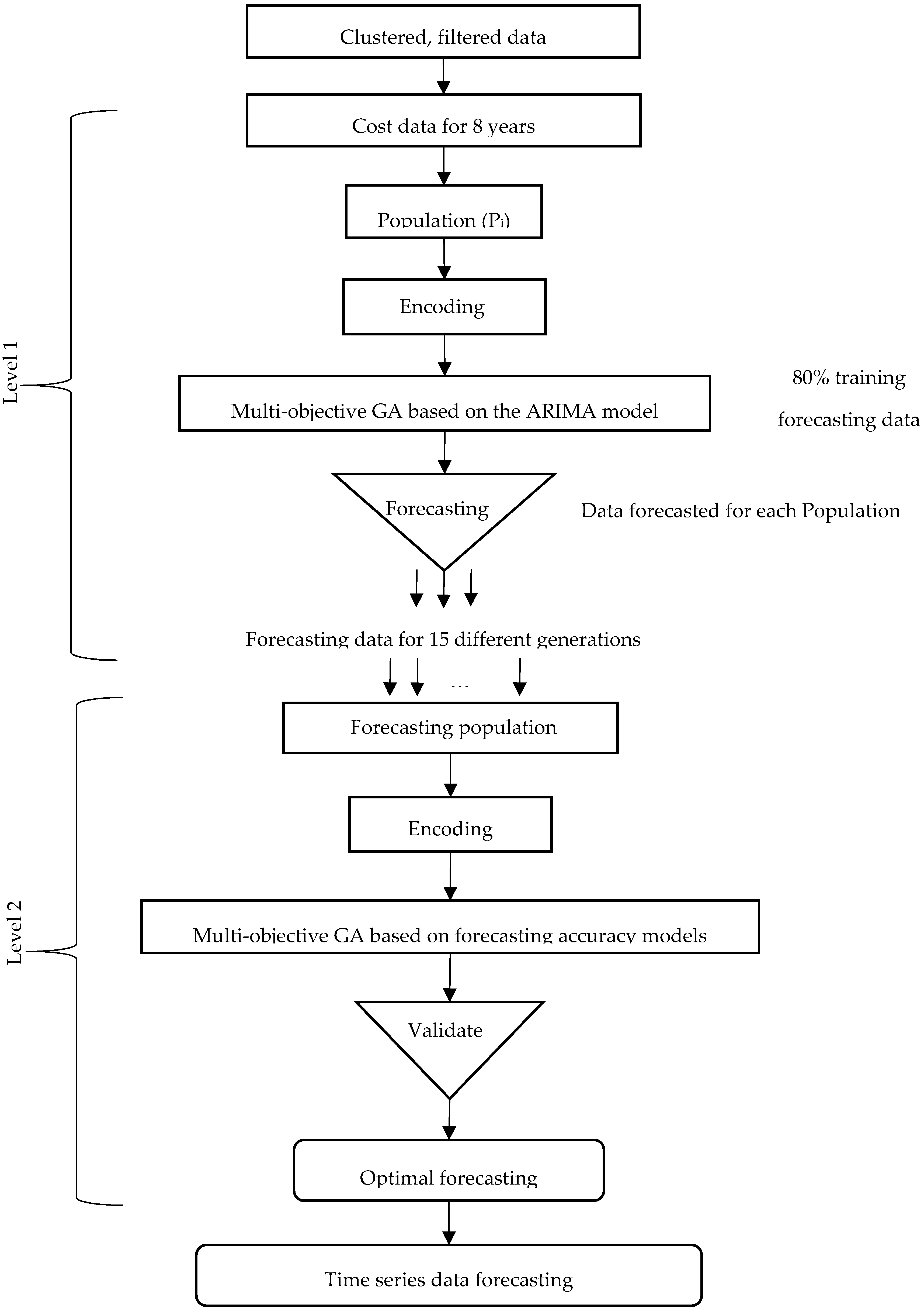
2.3. Two-Level System of Multi-Objective Genetic Algorithms

In this study, a novel two-level multi-objective GA has been developed, as shown in Figure 1. The levels of the GA are as follows: (1) a multi-objective GA based on the ARIMA model for forecasting the cost data, and (2) a multi-objective GA based on multiple functions for measuring the forecasting accuracy for validation of the forecasted data. Level 1 of the multi-objective GA is applied to the cost data objects (labour and material) at four different times (four populations) to forecast data for the next level and for each of 15 different generations. The second level validates the forecasted data for the two cost objects. Using two levels allows us to reduce the computational cost [17], while reaching an effective and reasonable solution [18].

2.3.1. Level 1: Multi-Objective GA Based on the ARIMA Model

The proposed multi-objective GA method uses a particular optimization based on the principle of natural selection of the optimal solution and applies this optimization on a wide range of forecasting populations. The multi-objective GA creates populations of chromosomes as possible answers to estimate the optimum forecasting [6]. This algorithm is robust, generic and easily adaptable because it can be broken down into the following steps: initialization, evaluation, selection, crossover, mutation, update and completion. The evaluation (fitness function) step creates the basis for a new population of chromosomes. The new population is formed using specific genetic operators, such as crossover and mutation [19,20]. The fitness function is derived from the ARIMA forecasting model. A GA with automated optimization avoids the weakness of the ARIMA model by estimating the parameters for forecasting [10].

The multi-objective GA is a global optimization technique that can be used to achieve an accurate forecasting based on the ARIMA model. The GA is known to help in solving complex nonlinear problems that often lead to cases where the search space shows a curvy landscape with numerous local minima. Moreover, the multi-objective GA is designed to find the optimal forecasting solution through automated optimization of the ARIMA model. In addition, the multi-objective GA can evaluate the forecasting accuracy using multiple fitness functions based on statistical models.

The first level utilises a multi-objective GA which is based on the ARIMA model and is implemented four different times using a cross-validation randomization technique. The technique aims to select the best time series data for forecasting. The process is the following: a random number of cost data are selected based on encoding in each of the four implementations; the modified random cost data are generated 15 times. The modifications are used to find the optimal cost data for forecasting. The following steps are implemented when applying the multi-objective GA in level 1.

Step 1: Initial population

A longitudinal study of each cost object ($Z^{labour}$, $Z^{material}$) is used to forecast data using the multi-objective GA for the two objects in parallel.

Step 2: First GA generation and selection

The first generation is performed by selecting each cost object and checking whether the data are stationary (i.e., trend-stationary) or non-stationary using a Dickey-Fuller test as in the Equation (2) [21]. To apply the ARIMA model, the data should be stationary, i.e., the null hypothesis of stationarity should not be rejected. When applying the Dickey-Fuller test equation, the hypothesis p = 1 means that the data are non-stationary and p < 1 that the data are stationary [21].

The Dickey-Fuller test equation is as in the Equation (2):

$$\mathrm{Dickey}-\mathrm{Fuller}\mathrm{test}(y_t)=\alpha +p{x}_{t-k}+{\epsilon }_t$$

(2)

where the notation is as follows:

• $y_t$: the actual data over time;
• $\alpha$: constant estimated value of the time series data;
• $p$: the hypothesis is either $p$ = 1 or $p$ < 1;
• $t$: time $\left\{1,\dots ,k\right\}$;
• $\epsilon$: the white noise of the time series data.

Step 3: Encoding

Random values, either ones or zeros, are generated for each cost data object. Encoding is the process of transforming from the phenotype to the genotype space before proceeding with multi-objective GA operators and finding the local optima.

Step 4: Fitness function

The fitness function in the Equation (3) is based on the ARIMA model for the forecasting of time series cost data objects individually, as seen in the equation below. The fitness function consists of an autoregression (AR) part and a moving average (MA) part [1]. The ARIMA model uses AR and MA polynomials to estimate $\left(p\right)$ and $\left(q\right)$ [1].

The fitness function is formulated as in the Equation (3):

$$fitness\left(p, d, q\right)=\mu +{\displaystyle \sum }_{i=1}^p\left(\sigma y_{t-1}\right)+{\displaystyle \sum }_{i-1}^q\left({\theta }_i{ϵ}_{t-1}\right)+{ϵ}_t$$

(3)

where the following notation is used:

• $\mu$: the mean value of the time series data;
• $p$: the number of autoregressive cut-off lags;
• $d$: the number of differences calculated with the equation $\Delta y_t=y_t-y_{t-1}$;
• $q$: the number of cut-off lags of the moving average process;
• $\sigma$: autoregressive coefficients (AR);
• $\theta$: moving average coefficients (MA);
• $t$: time $\left\{1,\dots ,k\right\}$;
• $ϵ$: the white noise of the time series data.

The parameters ($p,q$) are estimated using an autocorrelation function (ACF) and a partial autocorrelation function (PACF) [1]. The estimated values produced by the previous equation will be used to create a forecast for 20 months ($m$) using the Equation (4) [22]. These forecasted values will be evaluated using the second level of the multi-objective GA to find the optimal forecasting with high accuracy.

$$fitness\left(t+m\right)=\mu +{\displaystyle \sum }_{i=1}^p\left(\sigma y_{t-1}\right)+{\displaystyle \sum }_{i-1}^q\left({\theta }_i{ϵ}_{t-1}\right)+{ϵ}_t$$

(4)

where $fitness\left(t+m\right)$ is the time series forecasting at time $\left(t+m\right)$ and

• $m$: months {1, 2, 3,…, $m$}.

Step 5: Crossover and mutation

In this study, a one-point crossover with a fixed crossover probability is used. This probability decreases the bias of the results over different generations caused by the huge data values. For chromosomes of length $l$, a crossover point is generated in the range [1, 1/2$l$] and [1/2$l$, $l$]. The values of objects are connected and should be exchanged to produce two new offspring. We select two points to create more value ranges and find the best fit.

Randomly, ten percent of the selected chromosomes undergo mutation with the arrival of new chromosomes. For the cost object values, we swap two opposite data values. The purpose of this small mutation percentage is to keep the forecasting changes steady over different generations.

Step 6: New generation

The new generation step repeats steps 3–5 continuously for 15 generations. Fifteen generations are enough for these data because the curves of the fitness functions are repeated after fifteen generations. The selected fifteen generations are used individually for the second level to validate the forecasting accuracy for each object and population. This step yields fully correlated data for the next step.

2.3.2. Level 2: Multi-Objective GA for Measuring the Forecasting Accuracy

In this level, the multi-objective GA is applied longitudinally to the data. The multi-objective GA operates with a population of chromosomes that contains labour cost and material cost objects. The GA operates on the selected population over different generations to find the appropriate forecasting accuracy. During the GA generations, the chromosomes in the population are rated concerning their adaptation, and their mechanism of selection for the new population is evaluated. Their adaptability (fitness function) is the basis for a new population of chromosomes. The new population is formed using specific genetic operators such as crossover and mutation. The multi-objective GA is used to evaluate the forecasting accuracy for each generation of the first level.

Level 2 utilises a multi-objective GA which is based on different forecasting error rates and is implemented for each generation from the first level and for four different populations using a cross-validation randomization technique. This technique aims to select the best evaluation of the time series data forecasting and the process is as follows. A random number of cost data are selected based on the encoding in each generation of the four implementations, and the modified random cost data are generated five times. The modifications are then used to find the optimal cost data forecasting. In this study, due to the size of the training data, five generations are sufficient to obtain valid results. The following steps are implemented when applying the multi-objective GA in level 2.

Step 1: Initial population

A longitudinal study is performed of each generation and each cost object ($Z^{labour}$, $Z^{material}$) with its forecasted data using the multi-objective GA in parallel.

Step 2: First GA generation, encoding and selection

The first generation is performed by selecting each cost object and encoding through generating random values, either ones or zeros, for each cost data object. The selection for each cost data object is based on encodings with the value of 1. This selection is used to evaluate the forecasted data using the multi-objective fitness function.

Step 3: Fitness function

The multi-objective fitness function is based on multiple functions for measuring the forecasting accuracy. The mean absolute percentage error (MAPE), the median absolute percentage error (MdAPE), the root mean square percentage error (RMSPE), the root median square percentage error (RMdSPE), and the mean absolute scaled error (MASE) are different fitness functions used to evaluate the selected forecasting data from the previous step. The fitness functions are formulated as follows in the Equations (5)–(9) [23]:

$$fitness\left(MAPE\right)=mean\left(\left|p_t\right|\right)$$

(5)

where $p_t=\frac{100e_t}{Y_i}$ and $e_t=Y_t-F_t$

$$fitness\left(MdAPE\right)=median\left(\left|p_t\right|\right)$$

(6)

where $p_t=\frac{100e_t}{Y_i}$ and $e_t=Y_t-F_t$,

$$fitness\left(RMSPE\right)=\sqrt{mean\left(p_t^2\right)}$$

(7)

where $p_t=\frac{100e_t}{Y_i}$ and $e_t=Y_t-F_t$

$$fitness\left(RMdSPE\right)=\sqrt{median\left(p_t^2\right)}$$

(8)

where $p_t=\frac{100e_t}{Y_i}$ and $e_t=Y_t-F_t$

$$fitness\left(MASE\right)=mean\left(\left|q_t\right|\right)$$

(9)

where $q_t=\frac{e_t}{\frac{1}{n-1}{{\displaystyle \sum }}_{i=2}^n\left|Y_i-Y_{i-1}\right|}$, where $e_t=Y_t-F_t$;

In the above equations, the following notation is used:

• $t$: time $\left\{1,\dots ,k\right\}$;
• $Y_t$: the actual data over time;
• $F_t$: the forecasted data over time.

The MAPE is often substantially larger than the MdAPE when the data involve small counts. In this study, it was impossible to use these measures since zero values of $Y_t$ frequently occurred. The RMSPE and RMdSPE are more sensitive to the data. These methods are examples of a random walk and measure the accuracy based on the last adjusted observation of forecasted seasonality. The MASE is a scaled measure based on relative errors. This module tries to remove the scale of the data by comparing the forecasted data with data obtained from some benchmark forecast method [23].

Step 4: Crossover and mutation

In this study, we use a one-point crossover with a fixed crossover probability. This probability decreases the bias of the results over different generations due to the huge data values. For chromosomes of length $l$, a crossover point is generated in the range [1, 1/2$l$] and [1/2$l$, $l$]. The values of objects are connected and should be exchanged to produce two new offspring. We select two points to create more value ranges and find the best fit.

Randomly ten percent of the selected chromosomes undergo mutation with the arrival of new chromosomes. For the cost object values, we swap two opposite data values. The purpose of this small mutation percentage is to keep the forecasting changes steady over different generations.

Step 5: New generation

The new generation step repeats steps 2 to 4 continuously for five generations. Five generations are enough for these data, because the fitness function is repeated after the fifth generation. The selected generation is used for the second level to validate the forecasting accuracy for each object. This step yields fully correlated data that can be used for forecasts covering several months.

2.4. Multi-Objective Genetic Algorithms (GAs) Based on the Dynamic Regression Model

The study has developed a multi-objective GA based on the dynamic regression model. The dynamic regression (DR) model differs from the ordinary regression model in that it can handle both contemporaneous and time-lagged relationships [24]. A dynamic model is a family of functions of the data, of relatively simple form and devised by a researcher to produce more realistic results. In addition, this model emphasizes the ripple effect which the input variables can have on the dependent variables. Therefore, the DR model is one of the interspersing models to be compared with the ARIMA model as one of the most popular models for forecasting. The developed GA consists of the following levels: (1) a multi-objective GA based on the DR model and used to forecast cost data, and (2) a multi-objective GA based on multiple functions for measuring the forecasting accuracy for the purpose of validating the forecasted data. The multi-objective GA is applied to the cost data objects (labour and material) for 15 different generations for four different populations to forecast data for the next level. Then the forecasted data for the two cost objects are validated.

We use the same steps as those applied in the first level of the GA based on the ARIMA model, applying them on the same data with the same method for every step. However, the fitness function step is based on the regression model, as clarified below.

Step 3: Fitness function

The multi-objective fitness function is based on the DR model function, as expressed in the fitness Equation (11) [24]. The fitness function is applied to a 20-month forecast. The data have been normalized before calculating the fitness function. The purpose of the normalization is to decrease the computation complexity, since the cost data values are huge. The equation used for the normalization $\overline{Y}$ as in the Equation (10) [25]:

$$\overline{Y}=(Y_t-mi{n}_{Y_t}) / \left(ma{x}_{Y_t}-mi{n}_{Y_t}\right)$$

(10)

The fitness equation is as the Equation (11) [24]:

$$\mathrm{fitness}\left(Y_t\right)=C+b_1{Y}_{t-1}+b_1{Y}_{t-2}+WN$$

(11)

where the notation is as follows:

• $C$: constant value calculated with the normal equation, where $X^{T}XA=X^{T}b$;
• $b_1$ and $b_2$: calculated with the normal equation, where $X^{T}XA=X^{T}b$;
• $Y_t$: related to $Y_{t-1}$ and $Y_{t-2}$;
• $WN$: white noise.

The results of the fitness function for the 20-month forecast are denormalized to the original data using the Equation (12) [25]. The denormalization values are used to evaluate the forecasting accuracy using the second level.

$$Y_t=\overline{Y}\ast \left(ma{x}_{Y_t}-mi{n}_{Y_t}\right)+mi{n}_{Y_t}$$

(12)

The forecasting accuracy for every generation for every population is validated using the multi-objective GA based on multiple functions for measuring the forecasting accuracy. The mean absolute percentage error (MAPE), the median absolute percentage error (MdAPE), the root mean square percentage error (RMSPE), the root median square percentage error (RMdSPE), and the mean absolute scaled error (MASE) are different fitness functions used to evaluate the selected forecasting data from the previous step [23]. The method used for validating the forecasting accuracy of the GA based on the ARIMA model is used to validate the forecasting accuracy of the GA based on the DR model.

2.5. Models Evaluation Method

A comparison of the three methods described above is performed based on the averages of the historical data, the actual data and the polynomial trends. The polynomial trend is often used in many applications and it was used in this study for the comparison of the models. Polynomial trending describes a pattern that represents data with many fluctuations over the time line. The formula of polynomial is presenting in each figure. The deviation average of $Y_t$ is calculated based on two different functions for every method. This provides a means of comparing the different methods and finding a proper forecasting, i.e., a forecasting where the deviation average is close to zero. This step confirms our judgement on the best forecasting method for the data.

For each method and cost data object, the average is calculated for the historical data, $A$, the actual data, $B$, the forecasted data, $C$, and the polynomial data, $D$. Figure 2 and Figure 3 show the averages calculated for the two cost objects of labour and materials. The average of the historical data (A) is the average of the data before the vertical line. The average of the actual data (B) is the average of the data after the vertical line. The average of the forecasted data (C) is the average of the forecasted data after the vertical line. The average of the polynomial data (D) is the average of the polynomial data after the vertical line. The following Equations (13) and (14) express the deviation average for each cost object:

$$\mathrm{deviation}\mathrm{average} \mathrm{DV}1 \left(Y_t\right)=\frac{B-C}{A}$$

(13)

$$\mathrm{deviation}\mathrm{average}\mathrm{DV}2 \left(Y_t\right)=\frac{B-D}{A}$$

(14)

$Y_t$ is the cost data object over $t$ time.

Each method has been developed using Python programing language and implemented on a server with special specifications to get the results. The server used in this study has 16 processors of E5-2690V2 (25M cash), 128 GB of RAM, 300 GB of Hard disk, and Windows-10 Enterprise 64 bit.

3. Results and Discussion

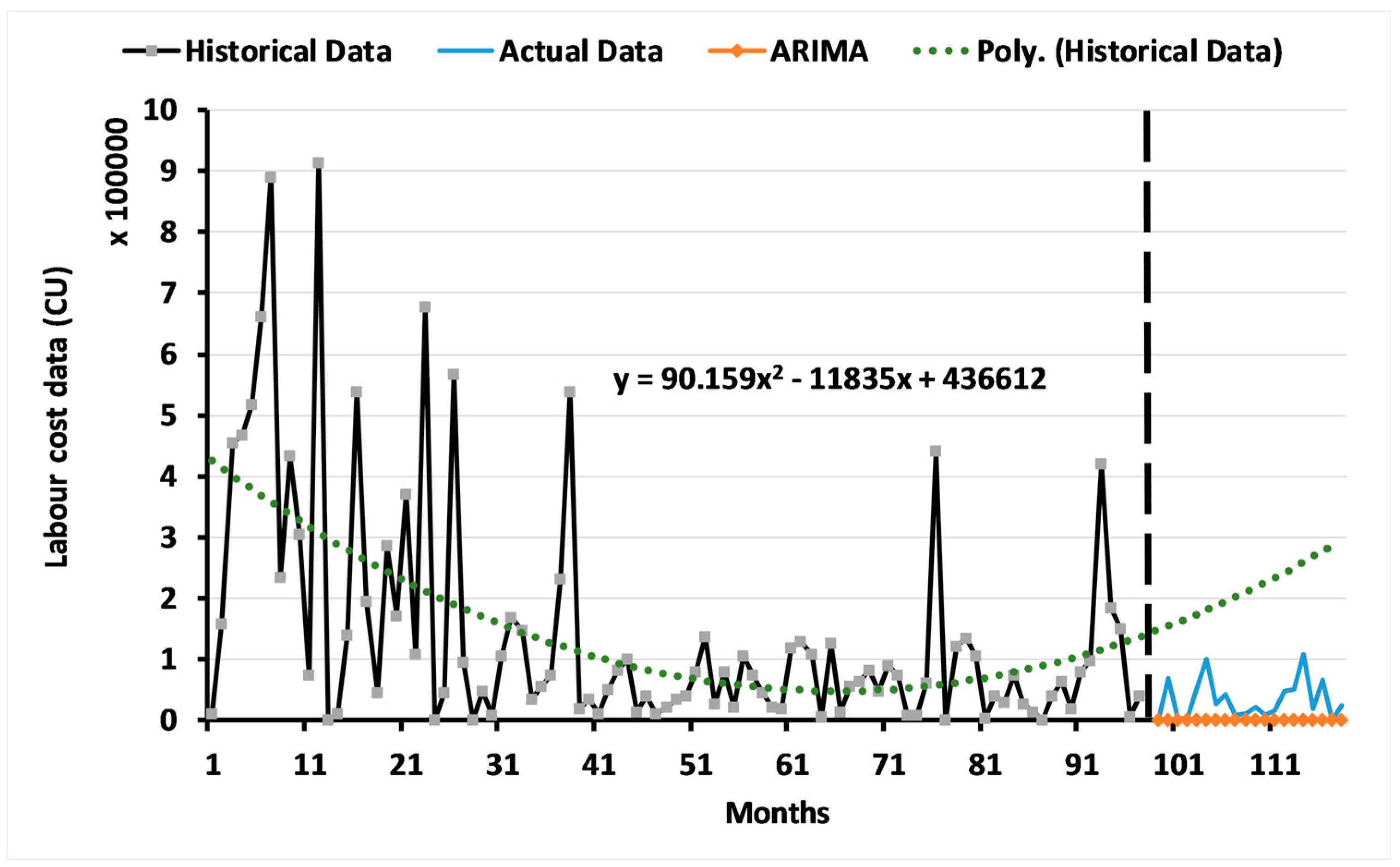
3.1. Results of the ARIMA Model

The ARIMA model was implemented stochastically based on the default values for the parameters $p$, $d$ and $q$ for the different scenarios and individually for each cost object ($Z^{labour}$, $Z^{material}$). The values assumed for each parameter in the scenarios were (1,1,1), (1,0,0), (1,0,1) and (2,0,1). For every scenario, all the cost data points of each object were included, covering a period of 97 months. The scenarios do not show a reasonable forecasting for a period of 20 months for each object. In this section, we present the cost object forecasting of the ARIMA model (1,1,1) as the default input parameters.

Figure 2 shows the forecasting for the labour cost object with the polynomial trend to illustrate the relationship between the values over a timeline with monthly intervals. Before the vertical line, the historical labour cost data for 97 months are shown, and after the vertical line, the actual labour cost data for 20 months are shown. The forecasted data for the 20-month period do not seem to be in sync with the actual data and are lower than the trend of the data. The forecasting based on the ARIMA model does not reflect the real data for the labour cost object.

Figure 3 shows the forecasting for the material cost object with the polynomial trend to illustrate the relationship between the values over a timeline with monthly intervals. Before the vertical line, the historical material cost data for 97 months are presented, and after the vertical line, the actual material cost data for 20 months are presented. The forecasted data for the 20-month period do not seem to be in sync with the actual data and are lower than the trend of the data. The forecasting based on the ARIMA model does not reflect the real data for the material cost object.

Overall, the forecasting based on the ARIMA model does not show sufficient accuracy over the 20-month period.

3.2. Results of the Two-Level System of Multi-Objective GAs

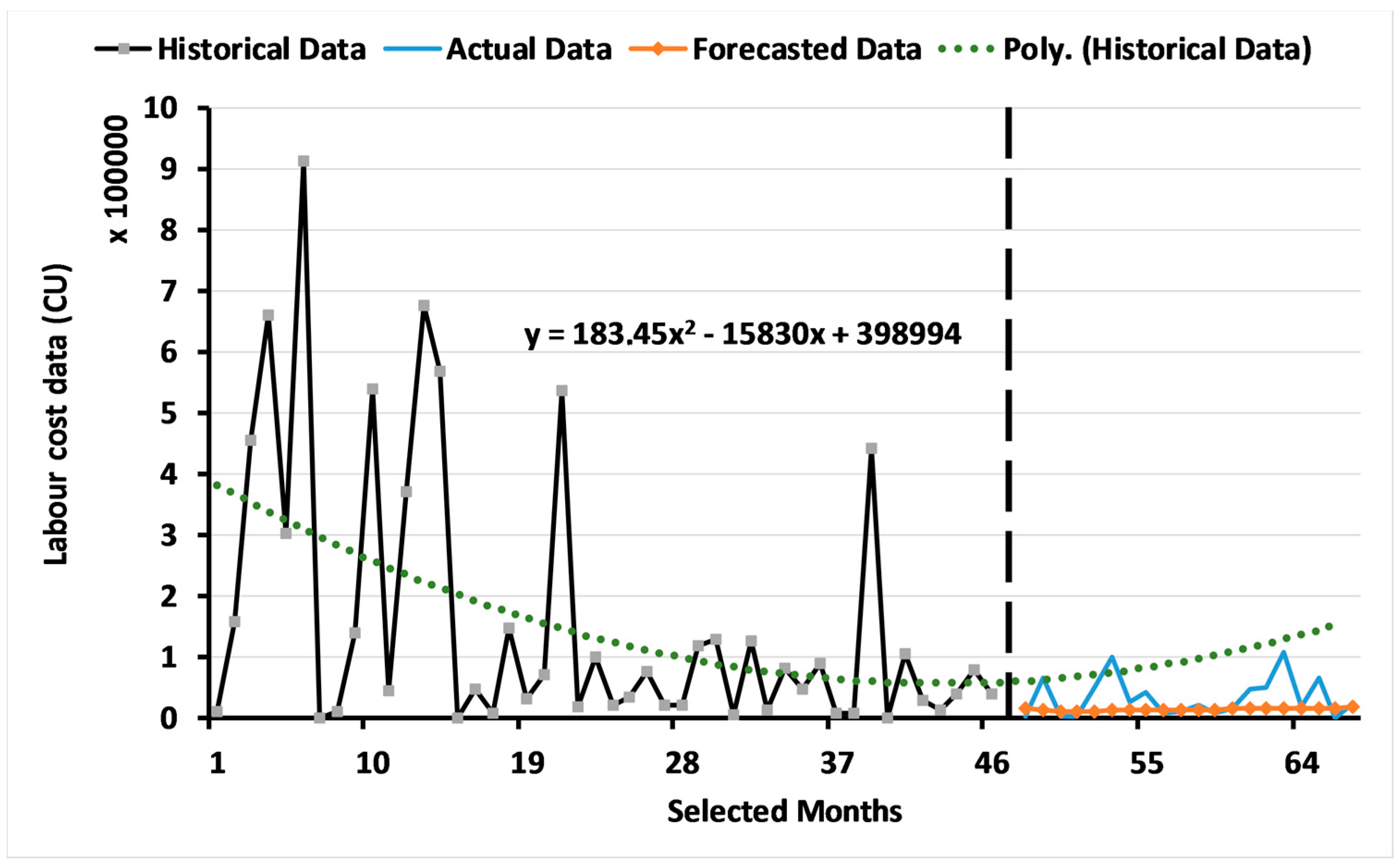
3.2.1. Results for Level 1: Multi-Objective GA Based on the ARIMA Model

In this part of the study, we tested four populations individually using the multi-objective GA based on the ARIMA model to generate forecasting data for the two different cost objects. The forecasted data for each population obtained with 15 different generations were then evaluated using the second level. The second level evaluation helped in deciding the best generation of the forecasted data. In this section, we present only the best forecasted curves with the historical data because of the huge number of possibilities considered in this study.

Figure 4 shows the forecasted labour data curve for 20 months from 2013 to 2015, for the second population and, specifically, for generation 13. In addition, it shows the historical data with the polynomial trend to illustrate the relationship between the independent variables over a timeline with monthly intervals. The selected labour data show a better forecasting than that obtained with the ARIMA model in that the forecasted data are close to the actual data and the polynomial trend. The ARIMA parameters for the selected labour cost data covering 47 months were $p=$ 0.22, $d=$ 1 and $q=$ 0.23.

Figure 5 shows the curve for the forecasted material data for 20 months from 2013 to 2015, for the third population and, specifically, for generation 10. In addition, this figure shows the original data with the polynomial trend to illustrate the relationship between the independent variables over a timeline with monthly intervals. The selected material data show better forecasting than that obtained with the ARIMA model in that the forecasted data are close to the actual data and the polynomial trend. The ARIMA parameters for the selected material cost data covering 52 months were $p=$ 0.39, $d=$ 1 and $q=$ 0.43.

The forecasted data for the labour and material cost objects were evaluated using the second level, applying a multi-objective GA based on the statistical forecasting error rate. The model for the forecasting accuracy evaluated the forecasted data for 20 months from 2013 to 2015 based on the actual values of this period. Implementing level 2, the accurate forecasted data were found, i.e., the proper selection of data for each object to be used for forecasting.

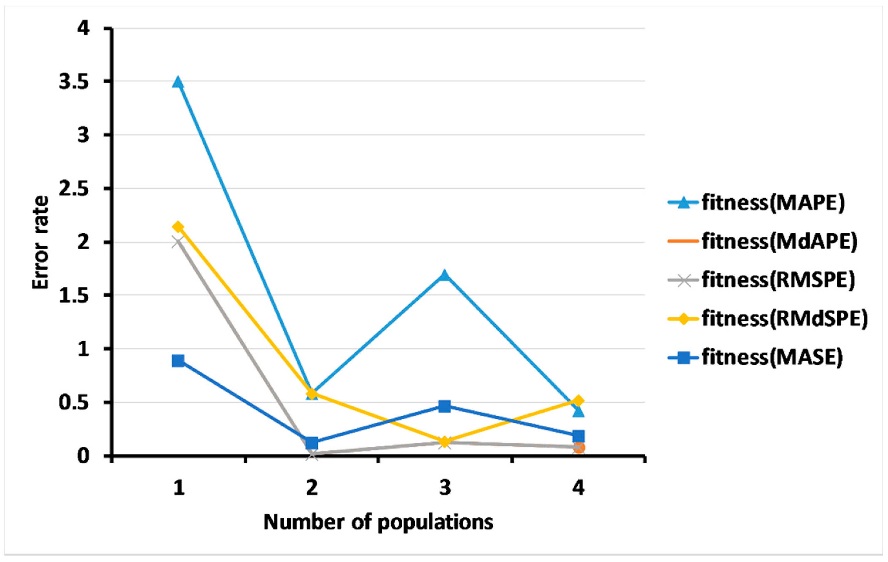
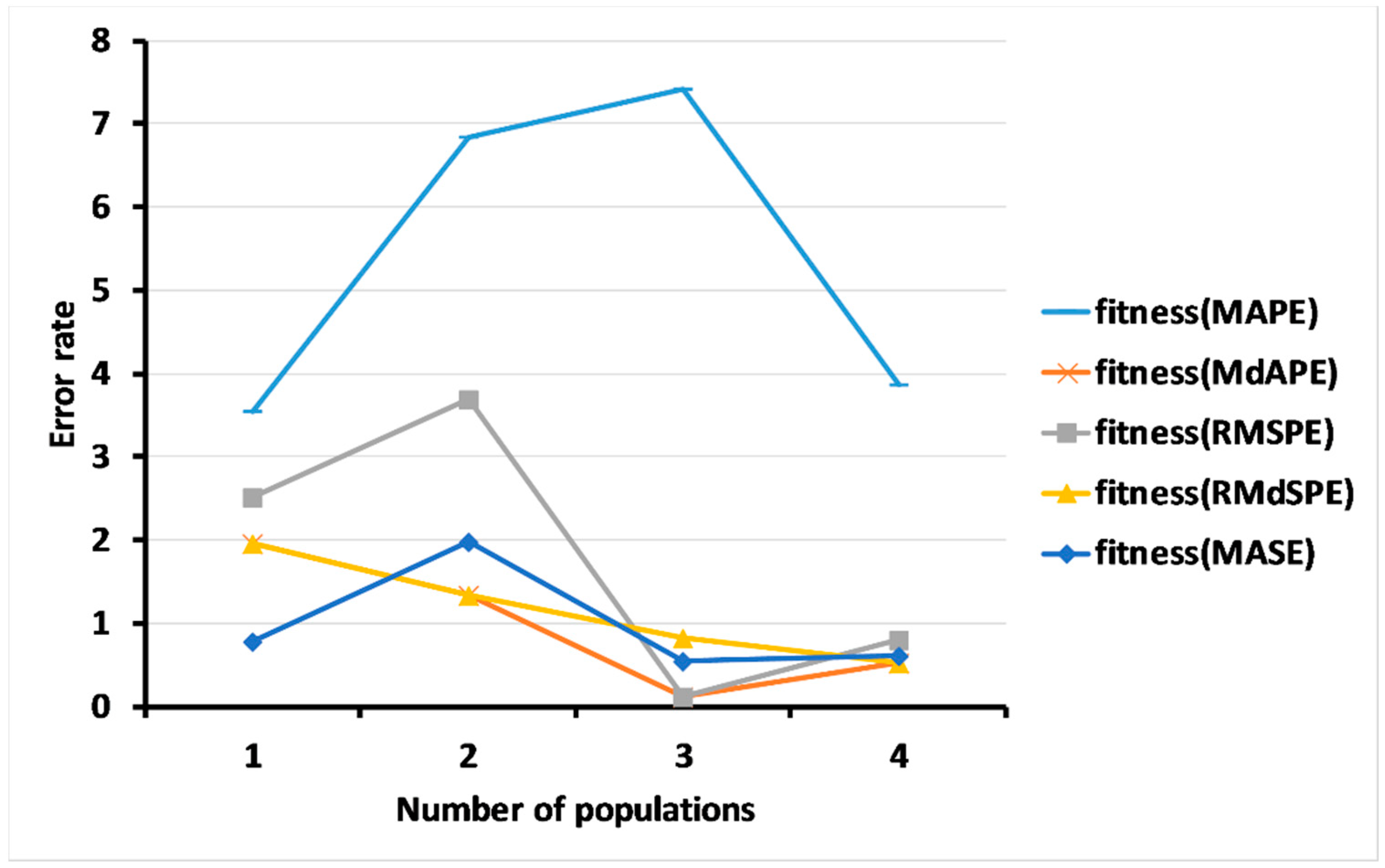
3.2.2. Results of Level 2: Multi-Objective GA for Measuring the Forecasting Accuracy

The outcome from the first level, specifically for each generation for each population, indicates the forecasting accuracy for each cost object. For each generation, the multi-objective GA based on multiple fitness functions was used to find the best fitness value through five different generations. The fitness functions (forecasting error rate models) provide an accurate data forecasting through comparing the behaviour of the different models and revealing which forecasting model is appropriate.

Figure 6 and Figure 7 show the forecasting accuracy for the labour and material cost objects obtained with five different fitness functions for the four populations. The fitness function values of each population are the minimum values obtained through testing five different generations from the first level. Figure 6 shows the fitness values for the labour cost object. The figure shows five different curves for five different fitness functions.

Concerning the first population, $fitness\left(MAPE\right)$ has the highest error rate, 3.5, while $fitness\left(MdAPE\right)$ and $fitness\left(RMSPE\right)$ have the same value, 2.01. $fitness\left(RMdSPE\right)$ has a value of 2.15 and $fitness\left(MASE\right)$ has the lowest value, 0.89. Concerning the second population, $fitness\left(MdAPE\right)$ and $fitness\left(RMSPE\right)$ show the same value, 0.02, which is the lowest fitness value for this population. The value for $fitness\left(MASE\right)$ is 0.12, while the values for $fitness\left(RMdSPE\right)$ and $fitness\left(MAPE\right)$ are 0.58 and 0.59, respectively.

Concerning the third population, $fitness\left(MdAPE\right)$ and $fitness\left(RMSPE\right)$ show the same value, 0.13, which is the lowest fitness value for this population. The value for $fitness\left(RMdSPE\right)$ is 0.14, which is higher than that for $fitness\left(MdAPE\right)$ and $fitness\left(RMSPE\right)$, while the values for $fitness\left(MASE\right)$ and $fitness\left(MAPE\right)$ are 0.47 and 1.7, respectively. Finally, concerning the fourth population, $fitness\left(MdAPE\right)$ and $fitness\left(RMSPE\right)$ show the same value, 0.08, which is the lowest fitness value for this population. $fitness\left(MASE\right)$ has a value of 0.19, while $fitness\left(MAPE\right)$ and $fitness\left(RMdSPE\right)$ have higher values, 0.43 and 0.52, respectively.

Overall, the fitness functions are variants. $fitness\left(MAPE\right)$ has the highest of all the curves of the four populations because it involves small data counts. $fitness\left(MdAPE\right)$ and $fitness\left(RMSPE\right)$ have almost equal values over the four populations, while their values can be regarded as almost close when one takes all the 15 generations for the four populations into account. The $fitness\left(RMdSPE\right)$ and $fitness\left(MASE\right)$ curves show a sensitivity to the data caused by the population randomization.

Selecting a proper population for the labour cost data is quite difficult due to the variety of fitness values. In this study, we considered the population that was selected by more than two of the fitness functions to have a low forecasting error rate. The thirteenth generation for the second population was selected as having the lowest forecasting error rate with a suitable selection of input data. The labour cost data were selected using three fitness functions, $fitness\left(MdAPE\right)$, $fitness\left(RMdSPE\right)$ and $fitness\left(MASE\right),$ with values of 0.02, 0.02 and 0.12, respectively.

Figure 7 shows the fitness values for the material cost object. The figure shows that, concerning the first population, $fitness\left(MAPE\right)$ has the highest error rate, 3.54, while $fitness\left(MdAPE\right)$ and $fitness\left(RMdSPE\right)$ have the same value, 1.97. $fitness\left(RMSPE\right)$ has a value of 2.54 and $fitness\left(MASE\right)$ has the lowest value, 0.79. With regard to the second population, $fitness\left(MdAPE\right)$ and $fitness\left(RMdSPE\right)$ show the same value, 1.35, which is the lowest fitness value for this population. The value for $fitness\left(MASE\right)$ is 1.99, while the values for $fitness\left(RMSPE\right)$ and $fitness\left(MAPE\right)$ are 3.7 and 6.84, respectively.

With regard to the third population, $fitness\left(MdAPE\right)$ and $fitness\left(RMSPE\right)$ show the same value, 0.13, which is the lowest fitness value for this population. The values for $fitness\left(RMdSPE\right)$ and $fitness\left(MASE\right)$ are 0.82 and 0.55, respectively. The value for $fitness\left(MAPE\right)$ is 7.42, which is the highest value for the third population. Concerning the fourth population, $fitness\left(MdAPE\right)$ and $fitness\left(RMdSPE\right)$ have the same value, 0.52, which is the lowest fitness value of this population. The value for $fitness\left(RMSPE\right)$ is 0.8, while the values for $fitness\left(MASE\right)$ and $fitness\left(MAPE\right)$ are 0.61 and 3.87, respectively; 3.87 is the highest value for this population.

The fitness functions are variants. The curve of $fitness\left(MAPE\right)$ is the highest of all the curves of the four populations. $fitness\left(MdAPE\right)$ and $fitness\left(RMdSPE\right)$ have almost equal values over the four populations. The $fitness\left(RMSPE\right)$ and $fitness\left(MASE\right)$ curves show sensitivity to the data according to the populations. Selecting a proper population for the material cost data is also quite difficult due to the variety of fitness values. In this study, we considered the population that was selected by more than two of the fitness functions to have a low forecasting error rate. The tenth generation for the third population was selected as having the lowest forecasting error rate with a suitable selection of input data. The material cost data were selected using three fitness functions, $fitness\left(MdAPE\right)$, $fitness\left(RMSPE\right)$ and $fitness\left(MASE\right),$ with fitness values of 0.13, 0.13 and 0.55, respectively.

The multiple fitness functions used in the second level helped in evaluating the forecasted data and in making a judgement on the forecasting method for each object. These models have different sensitivity to the data depending on the calculation method. Therefore, considering all of them is important to find a proper population for forecasting and then a proper generation of data.

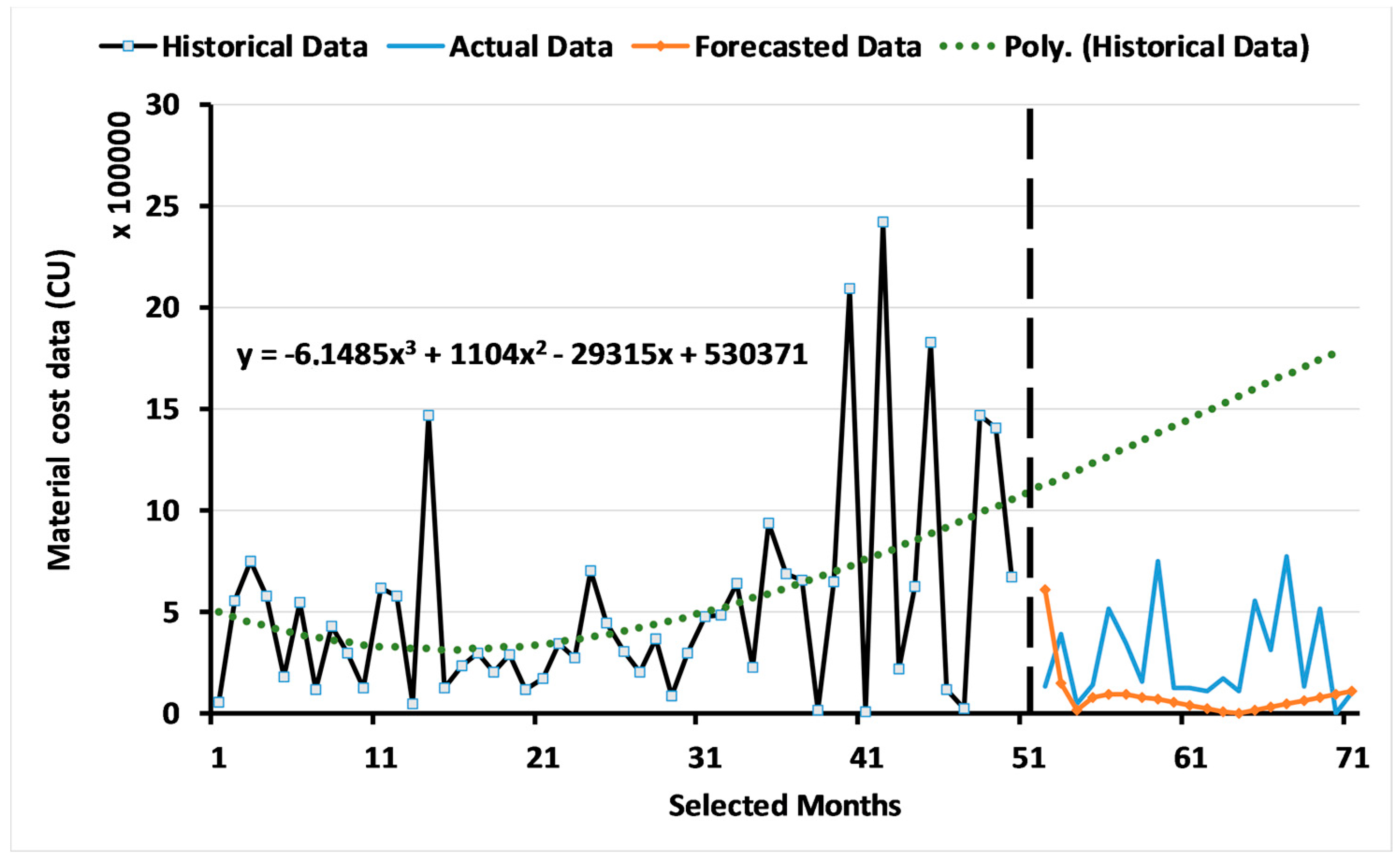
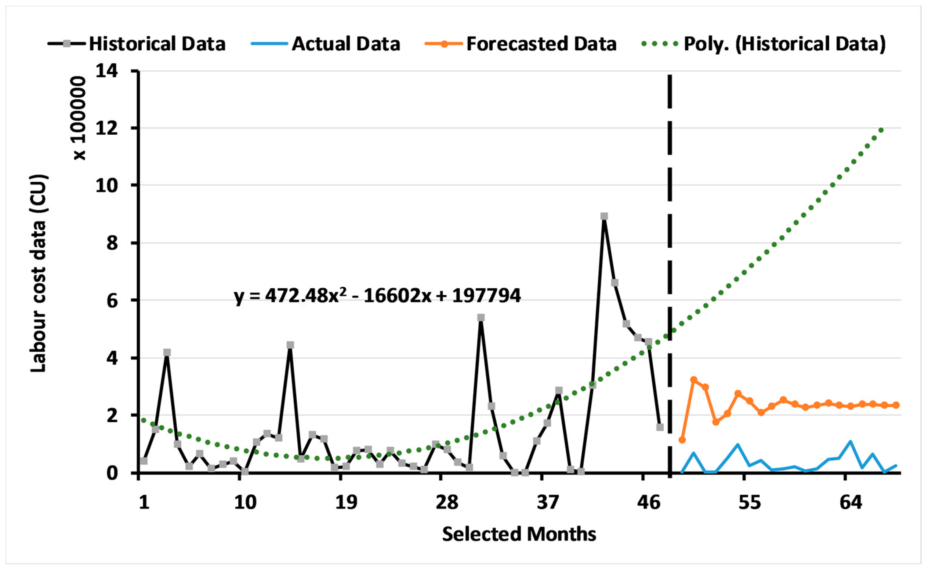
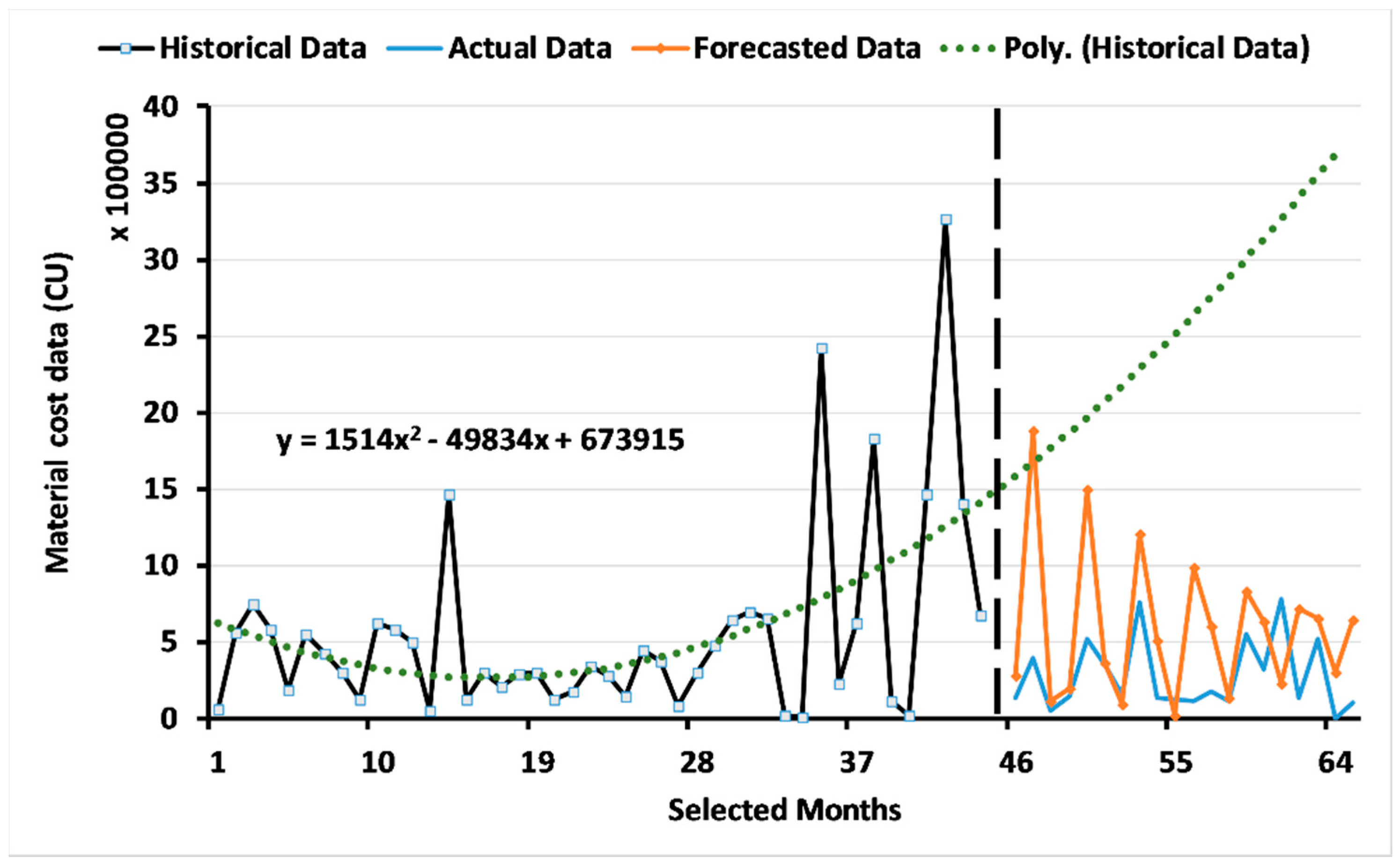
3.3. Results of the Multi-Objective Genetic Algorithms (GAs) Based on the Dynamic Regression Model

The outcome from this model, specifically for each generation for each population, indicates the accuracy of the forecasted values for each cost object. For each generation, the fitness functions of the second level provide an assessment of the data forecasting, assure the accuracy of the forecasting and reveal which forecasting model is appropriate. The forecasted data for the labour and material cost objects were evaluated in the second level using the multi-objective GA based on the statistical forecasting error rate. The model for the forecasting accuracy evaluated the forecasted data for 20 months from 2013 to 2015 based on the actual values of this period.

Figure 8 shows the curve of the forecasted labour data for 20 months from 2013 to 2015, for the fourth population and, specifically, for generation 2. The figure shows the historical data with the polynomial trend to illustrate the relationship between the independent variables over a timeline with monthly intervals. The selected labour data do not show a fit between the forecasted data, the actual data and the polynomial trend. Three of the forecasting accuracy functions, $fitness\left(MAPE\right)$, $fitness\left(MdAPE\right)$ and $fitness\left(RMdSPE\right),$ have the same minimum forecasting error rate, 0.9. In addition, the minimum error rate for $fitness\left(MASE\right)$ is 0.19.

Figure 9 shows the curve of the forecasted material data for 20 months from 2013 to 2015, for the third population and, specifically, for generation 12. The figure shows the historical data with the polynomial trend to illustrate the relationship between the independent variables over a timeline with monthly intervals. The selected material data do not show a fit between the forecasted data, the actual data and the polynomial trend. Three of the forecasting accuracy functions, $fitness\left(MAPE\right)$, $fitness\left(MdAPE\right)$ and $fitness\left(RMdSPE\right)$, have the same minimum forecasting error rate, 0.9. In addition, the minimum error rate for $fitness\left(MASE\right)$ is 0.54.

3.4. Results of a Comparison of the Methods

Table 1. The deviation averages for the labour cost object for every method.

	DV1	DV2
ARIMA model	0.2374	1.2169
Multi-objective GA based on the ARIMA model	0.1192	0.3869
Multi-objective GA based on the dynamic regression model	1.2630	6.2324

and

Table 2. The deviation averages for the material cost object for every method.

	DV1	DV2
ARIMA model	0.4171	1.0438
Multi-objective GA based on the ARIMA model	0.3555	0.8477
Multi-objective GA based on the dynamic regression model	0.5615	3.9543

below show the deviation averages for the labour and material cost data for the three methods presented in this paper. The results presented in these tables confirm our judgement on the best method for forecasting cost data objects. Table 1 shows that, for the labour cost data, the lowest values for the deviation averages DV1 and DV2 were obtained with the multi-objective GA based on the ARIMA model. Table 2 shows that, for the material cost data, the lowest values for the deviation averages DV1 and DV2 were also obtained with the multi-objective GA based on the ARIMA model.

The literature cited present different methodologies for forecasting compared with our methods. Vantuch & Zelinka [11], Ervural et al. [13] and Hatzakis & Wallace [6] used GAs with the ARIMA model to improve results compared with use of the ARIMA model alone. These authors used GAs to obtain a randomization of the ARIMA parameters, which is not always sufficient because ARIMA parameter estimation should be based on the data and research problem to achieve better forecasting. In addition, these authors used only one evaluation for the forecasting accuracy. Our method uses a GA to estimate the ARIMA parameters from the data and finds the best-fit model in forecasting. In addition, our method evaluates the forecasting accuracy using five different statistical fitness functions to achieve the optimal forecasting. The previously published studies have assumed that the data are accurate, while our study is based on clustered and improved data through imputing the missing data from other previous research [26].

Lin et al. [14] and Yu-Rong et al. [15] proposed a combination approach involving the BPNN and improved this approach by adopting a hybrid intelligent approach named the ADE-BPNN for time series forecasting. These authors used GA operators to improve the forecasting accuracy. These approaches have shown a relatively high accuracy, but have not been used for long-term forecasts and to process samples consisting of big data. Our model has a different integration of the ARIMA model with the GA and different GA operators to make it more suitable for the problem addressed in our research study. In addition, our model shows better performance when processing variant data samples and is able to make long-term forecasts.

Our model has been developed using Python as an open source programming language and the developed model can be used in different work environments with different systems. In the present study the model has been implemented on real cost data for a tunnel fan turbine system operated by Trafikverket. In addition, the model results show the achievement of optimal forecasting through GA variations and operations for short or long periods, in contrast to other methods. Trafikverket can use this model in forecasting different parameters with different data samples, systems or structures. The GA can adapt with the problem to achieve the purpose. To achieve the optimal solution, our model needs to be implemented on a server with the minimum specifications mentioned in Section 2.5.

4. Conclusions

In this study, it has been established that the ARIMA model and the multi-objective GA based on the dynamic regression model have drawbacks when used to forecast data for two cost objects. The data forecasted by the two models were not realistic and were not close to the actual data. The normalization performed in the multi-objective GA based on the dynamic regression model aims to decrease the computational complexity. However, this method does not achieve a better estimation of the parameters of the dynamic regression model and cannot be used for our data forecasting. The number of values produced in the model is huge, which somehow has a negative impact on the estimation of the parameters.

The multi-objective GA based on the ARIMA model provides other possibilities for calculating the parameters $\left(p,d,q\right)$ and improves the data forecasting. The outcome of the multi-objective GA based on the ARIMA model can be used to forecast data with a high level of accuracy, and the forecasted data can be used for LCC analysis.

References

1. Box, G.E.; Jenkins, G.M.; Reinsel, G.C.; Ljung, G.M. Time Series Analysis: Forecasting and Control; John Wiley & Sons: Hoboken, NJ, USA, 2015. [Google Scholar]
2. Tyralis, H.; Papacharalampous, G. Variable selection in time series forecasting using random forests. Algorithms 2017, 10, 114. [Google Scholar] [CrossRef]
3. Chen, Y.; Yang, B.; Dong, J.; Abraham, A. Time-series forecasting using flexible neural tree model. Inf. Sci. 2005, 174, 219–235. [Google Scholar] [CrossRef] [Green Version]
4. Hansen, J.V.; McDonald, J.B.; Nelson, R.D. Time Series Prediction with Genetic-Algorithm Designed Neural Networks: An Empirical Comparison With Modern Statistical Models. Comput. Intell. 1999, 15, 171–184. [Google Scholar] [CrossRef]
5. Ramos, P.; Oliveira, J.M. A Procedure for Identification of Appropriate State Space and ARIMA Models Based on Time-Series Cross-Validation. Algorithms 2016, 9, 76. [Google Scholar] [CrossRef]
6. Hatzakis, I.; Wallace, D. Dynamic multi-objective optimization with evolutionary algorithms: A forward-looking approach. In Proceedings of the 8th Annual Conference on Genetic and Evolutionary Computation, Seattle, WA, USA, 8–12 July 2006; pp. 1201–1208. [Google Scholar]
7. Ghaffarizadeh, A.; Eftekhari, M.; Esmailizadeh, A.K.; Flann, N.S. Quantitative trait loci mapping problem: An Extinction-Based Multi-Objective evolutionary algorithm approach. Algorithms 2013, 6, 546–564. [Google Scholar] [CrossRef]
8. Herbst, N.R.; Huber, N.; Kounev, S.; Amrehn, E. Self-adaptive workload classification and forecasting for proactive resource provisioning. Concurr. Comput. Pract. Exp. 2014, 26, 2053–2078. [Google Scholar] [CrossRef]
9. Kwiatkowski, D.; Phillips, P.C.; Schmidt, P.; Shin, Y. Testing the null hypothesis of stationarity against the alternative of a unit root: How sure are we that economic time series have a unit root? J. Econ. 1992, 54, 159–178. [Google Scholar] [CrossRef]
10. Hyndman, R.J.; Khandakar, Y. Automatic Time Series for Forecasting: The Forecast Package for R; Department of Econometrics and Business Statistics, Monash University: Clayton, VIC, Australia, 2007. [Google Scholar]
11. Vantuch, T.; Zelinka, I. Evolutionary based ARIMA models for stock price forecasting. In ISCS 2014: Interdisciplinary Symposium on Complex Systems; Springer: Berlin/Heidelberg, Germany, 2015; pp. 239–247. [Google Scholar]
12. Wang, C.; Hsu, L. Using genetic algorithms grey theory to forecast high technology industrial output. Appl. Math. Comput. 2008, 195, 256–263. [Google Scholar] [CrossRef]
13. Ervural, B.C.; Beyca, O.F.; Zaim, S. Model Estimation of ARMA Using Genetic Algorithms: A Case Study of Forecasting Natural Gas Consumption. Procedia-Soc. Behav. Sci. 2016, 235, 537–545. [Google Scholar] [CrossRef]
14. Wang, L.; Zeng, Y.; Chen, T. Back propagation neural network with adaptive differential evolution algorithm for time series forecasting. Expert Syst. Appl. 2015, 42, 855–863. [Google Scholar] [CrossRef]
15. Zeng, Y.; Zeng, Y.; Choi, B.; Wang, L. Multifactor-influenced energy consumption forecasting using enhanced back-propagation neural network. Energy 2017, 127, 381–396. [Google Scholar] [CrossRef]
16. Wang, L.; Wang, Z.; Qu, H.; Liu, S. Optimal forecast combination based on neural networks for time series forecasting. Appl. Soft Comput. 2018, 66, 1–17. [Google Scholar] [CrossRef]
17. Thomassey, S.; Happiette, M. A neural clustering and classification system for sales forecasting of new apparel items. Appl. Soft Comput. 2007, 7, 1177–1187. [Google Scholar] [CrossRef]
18. Ding, C.; Cheng, Y.; He, M. Two-level genetic algorithm for clustered traveling salesman problem with application in large-scale TSPs. Tsinghua Sci. Technol. 2007, 12, 459–465. [Google Scholar] [CrossRef]
19. Cordón, O.; Herrera, F.; Gomide, F.; Hoffmann, F.; Magdalena, L. Ten years of genetic fuzzy systems: Current framework and new trends. Fuzzy Sets Syst. 2001, 3, 1241–1246. [Google Scholar]
20. Shi, C.; Cai, Y.; Fu, D.; Dong, Y.; Wu, B. A link clustering based overlapping community detection algorithm. Data Knowl. Eng. 2013, 87, 394–404. [Google Scholar] [CrossRef]
21. Leybourne, S.J.; Mills, T.C.; Newbold, P. Spurious rejections by Dickey-Fuller tests in the presence of a break under the null. J. Econ. 1998, 87, 191–203. [Google Scholar] [CrossRef]
22. Huang, R.; Huang, T.; Gadh, R.; Li, N. Solar generation prediction using the ARMA model in a laboratory-level micro-grid. In Proceedings of the 2012 IEEE Third International Conference on Smart Grid Communications (SmartGridComm), Tainan, Taiwan, 5–8 November 2012; pp. 528–533. [Google Scholar]
23. Hyndman, R.J.; Koehler, A.B. Another look at measures of forecast accuracy. Int. J. Forecast. 2006, 22, 679–688. [Google Scholar] [CrossRef] [Green Version]
24. Hwang, S. Dynamic regression models for prediction of construction costs. J. Constr. Eng. Manag. 2009, 135, 360–367. [Google Scholar] [CrossRef]
25. Date, C.J. An Introduction to Database Systems; Pearson Education India: New Delhi, India, 2006. [Google Scholar]
26. Al-Douri, Y.; Hamodi, H.; Zhang, L. Data clustering and imputing using a two-level multi-objective genetic algorithms (GA): A case study of maintenance cost data for tunnel fans. Cogent Eng. 2018. submitted. [Google Scholar]
Figure 1. Two-level system of multi-objective GAs.
Algorithms 11 00123 g001
Figure 2. Labour cost data forecasting based on the ARIMA model.
Algorithms 11 00123 g002
Figure 3. Material cost data forecasting based on the ARIMA model.
Algorithms 11 00123 g003
Figure 4. Labour cost data forecasting using the multi-objective GA based on the ARIMA model.
Algorithms 11 00123 g004
Figure 5. Material cost data forecasting using the multi-objective GA based on the ARIMA model.
Algorithms 11 00123 g005
Figure 6. Labour cost error rate.
Algorithms 11 00123 g006
Figure 7. Material cost error rate.
Algorithms 11 00123 g007
Figure 8. Labour cost data forecasting based on the dynamic regression model.
Algorithms 11 00123 g008
Figure 9. Material cost data forecasting based on the dynamic regression model.
Algorithms 11 00123 g009