The Gradient and the Hessian of the Distance between Point and Triangle in 3D

Abstract

Computation of the distance between point and triangle in 3D is a common task in numerical analysis. The input values of the algorithm are coordinates of three points of the triangle and one point from which the distance is determined. An existing algorithm is extended to compute the gradient and the Hessian of that distance with respect to coordinates of involved points. Derivation of exact expressions for gradient and Hessian is presented, and numerical accuracy is evaluated for various cases. The algorithm has O(1) time and space complexity. The included open-source code may be used in applications where derivatives of point-triangle distance are required.

1. Introduction

The algorithm developed by Eberly [1] evaluates the distance function between a point and a triangle in 3D. The input parameters are coordinates of four points, which are involved in the point-triangle setup. Three points are vertices of the triangle, with the remaining point being the one to which the distance is computed. The motivation for this work is the need to obtain the gradient and the Hessian of that distance with respect to the input variables. Each of the four input points possesses three coordinates, giving 12 independent variables for the distance function. The distance function, accordingly, has 12 first derivatives and $12\times 12$ second derivatives, the components of the symmetric Hessian matrix.

Our approach is to differentiate the distance function provided by Eberly [1] and extend that algorithm with evaluation of first and second derivatives. The characteristics of the algorithm remain the same, i.e., the time and space complexity of the algorithm is O(1). A linear array of first derivatives and a 2D array of second derivatives are added to the output. The main contribution of the authors is the derivation of the expressions for the gradient and the Hessian of the distance. A potential application of this algorithm is in finding penetration penalty forces and their differentials for colliding polygonal objects in finite element (FE) simulations.

Numerical simulations of mechanical systems often involve contact interactions, and the penalty method is a common way of addressing this problem [2]. Implicit FE approaches rely on calculating derivatives of the forces generated in collisions, which in turn require first and second derivatives of the distance function. The FE simulation ARCSim [3] relies on penalty contact resolution for modeling deformation and fracture. ARCSim includes an approximation technique for obtaining the gradient and the Hessian of the distance function based on the surface normal of the interacting object. The approximation is not always accurate, which results in reduction of time steps, which sometimes halts the simulation.

In another method described by Fisher and Lin [4], the distance from the interior point to the surface of the object is precomputed on the nodes of interior polygonal mesh, representing a distance field. This discretized field allows one to estimate the spacial gradient of the distance. The accuracy is limited by the resolution of the mesh. In general, such approximation techniques are inaccurate, and there is a need for developing and utilizing the exact formula.

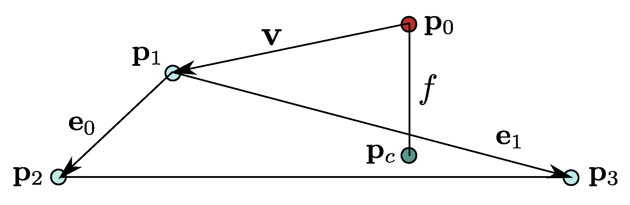
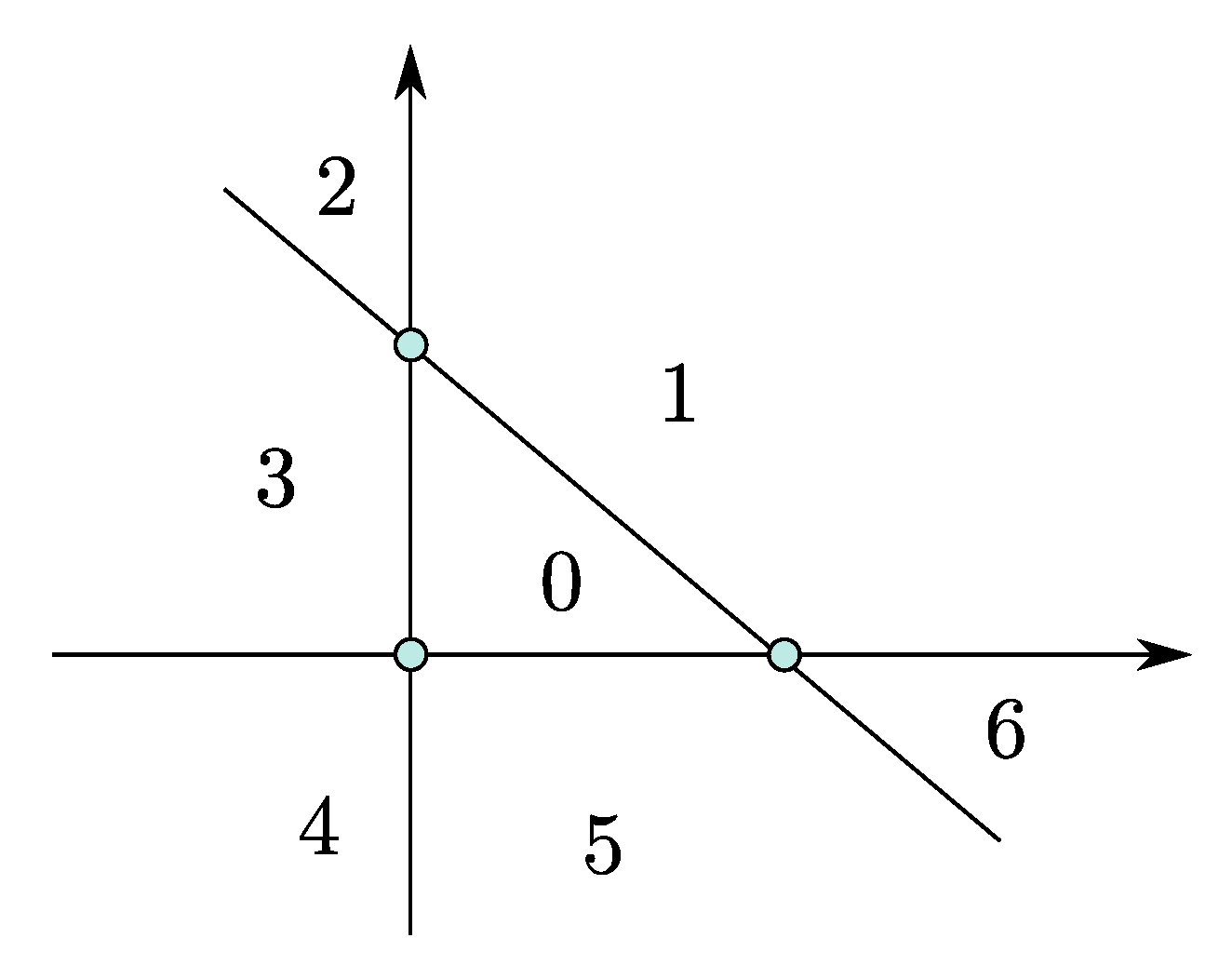
2. Mathematical Formulation

Figure 1 shows the point ${\mathbf{p}}_0(x_0,x_1,x_2)$ and the triangle with vertices ${\mathbf{p}}_1(x_3,x_4,x_5)$, ${\mathbf{p}}_2(x_6,x_7,x_8)$ and ${\mathbf{p}}_3(x_9,x_{10},x_{11})$. The projection point ${\mathbf{p}}_c$ has the barycentric coordinates ${\zeta }_1,{\zeta }_2,{\zeta }_3$:

$${\mathbf{p}}_c={\zeta }_1{\mathbf{p}}_1+{\zeta }_2{\mathbf{p}}_2+{\zeta }_3{\mathbf{p}}_3.$$

(1)

Figure 1. Distance f is determined between the point ${\mathbf{p}}_0$ and its projection ${\mathbf{p}}_c$ onto the triangle ${\mathbf{p}}_1{\mathbf{p}}_2{\mathbf{p}}_3$. Vectors ${\mathbf{e}}_0$, ${\mathbf{e}}_1$ and $\mathbf{v}$ are used in calculating f.

The squared distance between the point and the triangle is

$$s={\left|{\mathbf{p}}_0-{\mathbf{p}}_c\right|}^2=\sum _{k=0}^2{\left(x_k-\sum _{m=1}^3{\zeta }_m{x}_{k+3m}\right)}^2.$$

(2)

To obtain the gradient of s, Expression (2) is differentiated:

$$\frac{\partial s}{\partial x_i}=2\sum _{k=0}^2\left(x_k-\sum _{m=1}^3{\zeta }_m{x}_{k+3m}\right)\left({\delta }_{\left(k\right)\left(i\right)}-\sum _{m=1}^3\left({\zeta }_m{\delta }_{(k+3m)\left(i\right)}+x_{k+3m}\frac{\partial {\zeta }_m}{\partial x_i}\right)\right),$$

(3)

where ${\delta }_{ij}$ denotes the Kronecker symbol. Expressions for the barycentric coordinates ${\zeta }_m$ are given by Eberly [1], who introduces the following scalar coefficients:

$$a={\mathbf{e}}_0·{\mathbf{e}}_0,b={\mathbf{e}}_0·{\mathbf{e}}_1,c={\mathbf{e}}_1·{\mathbf{e}}_1,d={\mathbf{e}}_0·\mathbf{v},e={\mathbf{e}}_1·\mathbf{v},$$

(4)

where ${\mathbf{e}}_0={\mathbf{p}}_2-{\mathbf{p}}_1$, ${\mathbf{e}}_1={\mathbf{p}}_3-{\mathbf{p}}_1$ and $\mathbf{v}={\mathbf{p}}_1-{\mathbf{p}}_0$. The barycentric coordinates are then

$${\zeta }_1=1-({\zeta }_2+{\zeta }_3);{\zeta }_2=\frac{be-cd}{ac-b^2};{\zeta }_3=\frac{bd-ae}{ac-b^2}.$$

(5)

Expression (5) is used when ${\mathbf{p}}_c$ belongs to the interior region of the triangle. Cases when ${\mathbf{p}}_c$ belongs to an edge or coincides with one of the vertices are discussed in the next section. To obtain derivatives of ${\zeta }_2$ and ${\zeta }_3$, Expression (5) is differentiated:

$$\frac{\partial {\zeta }_2}{\partial x_i}=\frac{1}{\Delta }\left(e\frac{\partial b}{\partial x_i}+b\frac{\partial e}{\partial x_i}-d\frac{\partial c}{\partial x_i}-c\frac{\partial d}{\partial x_i}\right)-\frac{1}{{\Delta }^2}\frac{\partial \Delta }{\partial x_i}\left(be-cd\right),$$

(6)

$$\frac{\partial {\zeta }_3}{\partial x_i}=\frac{1}{\Delta }\left(d\frac{\partial b}{\partial x_i}+b\frac{\partial d}{\partial x_i}-e\frac{\partial a}{\partial x_i}-a\frac{\partial e}{\partial x_i}\right)-\frac{1}{{\Delta }^2}\frac{\partial \Delta }{\partial x_i}\left(bd-ae\right),$$

(7)

where $\Delta =ac-b^2$ and $\frac{\partial \Delta }{\partial x_i}=a\frac{\partial c}{\partial x_i}+c\frac{\partial a}{\partial x_i}-2b\frac{\partial b}{\partial x_i}$. Derivatives of ${\zeta }_1$ are

$$\frac{\partial {\zeta }_1}{\partial x_i}=-\left(\frac{\partial {\zeta }_2}{\partial x_i}+\frac{\partial {\zeta }_3}{\partial x_i}\right).$$

(8)

Coefficients $a,b,c,d,e$ (4) can be expanded in terms of $x_i$:

$$\begin{array}{c}a={(x_6-x_3)}^2+{(x_7-x_4)}^2+{(x_8-x_5)}^2,\hfill \\ b=(x_9-x_3)(x_6-x_3)+(x_{10}-x_4)(x_7-x_4)+(x_{11}-x_5)(x_8-x_5),\hfill & \hfill \\ c={(x_9-x_3)}^2+{(x_{10}-x_4)}^2+{(x_{11}-x_5)}^2,\hfill \\ d=(x_3-x_0)(x_6-x_3)+(x_4-x_1)(x_7-x_4)+(x_5-x_2)(x_8-x_5),\hfill & \hfill \\ e=(x_9-x_3)(x_3-x_0)+(x_{10}-x_4)(x_4-x_1)+(x_{11}-x_5)(x_5-x_2).\hfill & \hfill \end{array}$$

(9)

Then, gradients of Equation (9) are

$$\begin{array}{cc}\left[\frac{\partial a}{\partial x_i}\right]=2\times [0,0,0,x_3-x_6,x_4-x_7,x_5-x_8,x_6-x_3,x_7-x_4,x_8-x_5,0,0,0],\hfill & \hfill \\ \left[\frac{\partial b}{\partial x_i}\right]=[0,0,0,2x_3-x_6-x_9,2x_4-x_7-x_{10},2x_5-x_8-x_{11},x_9-x_3,x_{10}-x_4,\hfill & \hfill \\ x_{11}-x_5,x_6-x_3,x_7-x_4,x_8-x_5],\hfill & \hfill \\ \left[\frac{\partial c}{\partial x_i}\right]=2\times [0,0,0,x_3-x_9,x_4-x_{10},x_5-x_{11},0,0,0,x_9-x_3,x_{10}-x_4,x_{11}-x_5],\hfill \\ \left[\frac{\partial d}{\partial x_i}\right]=[x_3-x_6,x_4-x_7,x_5-x_8,x_0-2x_3+x_6,x_1-2x_4+x_7,x_2-2x_5+x_8,\hfill & \hfill \\ x_3-x_0,x_4-x_1,x_5-x_2,0,0,0],\hfill & \hfill \\ \left[\frac{\partial e}{\partial x_i}\right]=[x_3-x_9,x_4-x_{10},x_5-x_{11},x_0-2x_3+x_9,x_1-2x_4+x_{10},\hfill & \hfill \\ x_2-2x_5+x_{11},0,0,0,x_3-x_0,x_4-x_1,x_5-x_2].\hfill & \hfill \end{array}$$

(10)

Substituting Equation (10) into Equations (6) and (7) allows for obtaining $\frac{\partial s}{\partial x_i}$ in terms of $x_i$.

The second derivatives of s are procured in the same manner. First, Expression (3) is differentiated to obtain

$$\frac{{\partial }^{2}s}{\partial x_i\partial x_j}=2\sum _{k=0}^2\left({\left({\xi }^{\prime }\right)}^2+2\xi {\xi }^{″}\right),$$

(11)

where

$$\xi =x_k-\sum _{m=1}^3{\zeta }_m{x}_{k+3m},$$

(12)

$${\xi }^{\prime }={\delta }_{\left(k\right)\left(i\right)}-\sum _{m=1}^3\left({\zeta }_m{\delta }_{(k+3m)\left(i\right)}+x_{k+3m}\frac{\partial {\zeta }_m}{\partial x_i}\right),$$

(13)

$${\xi }^{″}=-\sum _{m=1}^3\left(\frac{\partial {\zeta }_m}{\partial x_j}{\delta }_{(k+3m)\left(i\right)}+\frac{\partial {\zeta }_m}{\partial x_i}{\delta }_{(k+3m)\left(j\right)}+x_{k+3m}\frac{{\partial }^2{\zeta }_m}{\partial x_i\partial x_j}\right).$$

(14)

Second derivatives of barycentric coordinates are obtained by differentiating Expressions (6) and (7):

$$\begin{array}{c}\hfill \frac{{\partial }^2{\zeta }_2}{\partial x_i\partial x_j}=\frac{1}{\Delta }\left(\frac{\partial b}{\partial x_j}\frac{\partial e}{\partial x_i}+\frac{\partial b}{\partial x_i}\frac{\partial e}{\partial x_j}-\frac{\partial c}{\partial x_j}\frac{\partial d}{\partial x_i}-\frac{\partial c}{\partial x_i}\frac{\partial d}{\partial x_j}\right)\\ \hfill +\frac{1}{\Delta }\left(e\frac{{\partial }^{2}b}{\partial x_j\partial x_i}+b\frac{{\partial }^{2}e}{\partial x_j\partial x_i}-d\frac{{\partial }^{2}c}{\partial x_j\partial x_i}-c\frac{{\partial }^{2}d}{\partial x_j\partial x_i}\right)\\ \hfill +\frac{1}{{\Delta }^2}\frac{\partial \Delta }{\partial x_j}\left(d\frac{\partial c}{\partial x_i}+c\frac{\partial d}{\partial x_i}-e\frac{\partial b}{\partial x_i}-b\frac{\partial e}{\partial x_i}\right)\\ \hfill +\frac{1}{{\Delta }^2}\frac{\partial \Delta }{\partial x_i}\left(d\frac{\partial c}{\partial x_j}+c\frac{\partial d}{\partial x_j}-e\frac{\partial b}{\partial x_j}-b\frac{\partial e}{\partial x_j}\right)\\ \hfill +\left(\frac{2}{{\Delta }^3}\frac{\partial \Delta }{\partial x_i}\frac{\partial \Delta }{\partial x_j}-\frac{1}{{\Delta }^2}\frac{{\partial }^2\Delta }{\partial x_i\partial x_j}\right)\left(be-cd\right),\end{array}$$

(15)

$$\begin{array}{c}\hfill \frac{{\partial }^2{\zeta }_3}{\partial x_i\partial x_j}=\frac{1}{\Delta }\left(\frac{\partial b}{\partial x_j}\frac{\partial d}{\partial x_i}+\frac{\partial b}{\partial x_i}\frac{\partial d}{\partial x_j}-\frac{\partial a}{\partial x_j}\frac{\partial e}{\partial x_i}-\frac{\partial a}{\partial x_i}\frac{\partial e}{\partial x_j}\right)\\ \hfill +\frac{1}{\Delta }\left(d\frac{{\partial }^{2}b}{\partial x_j\partial x_i}+b\frac{{\partial }^{2}d}{\partial x_j\partial x_i}-e\frac{{\partial }^{2}a}{\partial x_j\partial x_i}-a\frac{{\partial }^{2}e}{\partial x_j\partial x_i}\right)\\ \hfill +\frac{1}{{\Delta }^2}\frac{\partial \Delta }{\partial x_j}\left(e\frac{\partial a}{\partial x_i}+a\frac{\partial e}{\partial x_i}-d\frac{\partial b}{\partial x_i}-b\frac{\partial d}{\partial x_i}\right)\\ \hfill +\frac{1}{{\Delta }^2}\frac{\partial \Delta }{\partial x_i}\left(e\frac{\partial a}{\partial x_j}+a\frac{\partial e}{\partial x_j}-d\frac{\partial b}{\partial x_j}-b\frac{\partial d}{\partial x_j}\right)\\ \hfill +\left(\frac{2}{{\Delta }^3}\frac{\partial \Delta }{\partial x_i}\frac{\partial \Delta }{\partial x_j}-\frac{1}{{\Delta }^2}\frac{{\partial }^2\Delta }{\partial x_i\partial x_j}\right)\left(bd-ae\right),\end{array}$$

(16)

where $\frac{{\partial }^2\Delta }{\partial x_i\partial x_j}=\frac{\partial a}{\partial x_j}\frac{\partial c}{\partial x_i}+\frac{\partial a}{\partial x_i}\frac{\partial c}{\partial x_j}+c\frac{{\partial }^{2}a}{\partial x_i\partial x_j}+a\frac{{\partial }^{2}c}{\partial x_i\partial x_j}-2\frac{\partial b}{\partial x_i}\frac{\partial b}{\partial x_j}-2b\frac{{\partial }^{2}b}{\partial x_i\partial x_j}$. Similarly to Equation (8):

$$\frac{{\partial }^2{\zeta }_1}{\partial x_i\partial x_j}=-\left(\frac{{\partial }^2{\zeta }_2}{\partial x_i\partial x_j}+\frac{{\partial }^2{\zeta }_3}{\partial x_i\partial x_j}\right).$$

(17)

Second derivatives of the coefficients $a,b,c,d,e$ are constants that are included in Appendix A. The first and the second derivatives of the distance $f=\sqrt{s}$ are then expressed as:

$$\frac{\partial f}{\partial x_i}=\frac{1}{2\sqrt{s}}\frac{\partial s}{\partial x_i},$$

(18)

$$\frac{{\partial }^{2}f}{\partial x_i\partial x_j}=\frac{1}{2\sqrt{s}}\frac{{\partial }^{2}s}{\partial x_i\partial x_j}-\frac{1}{4s^{3/2}}\frac{\partial s}{\partial x_i}\frac{\partial s}{\partial x_j}.$$

(19)

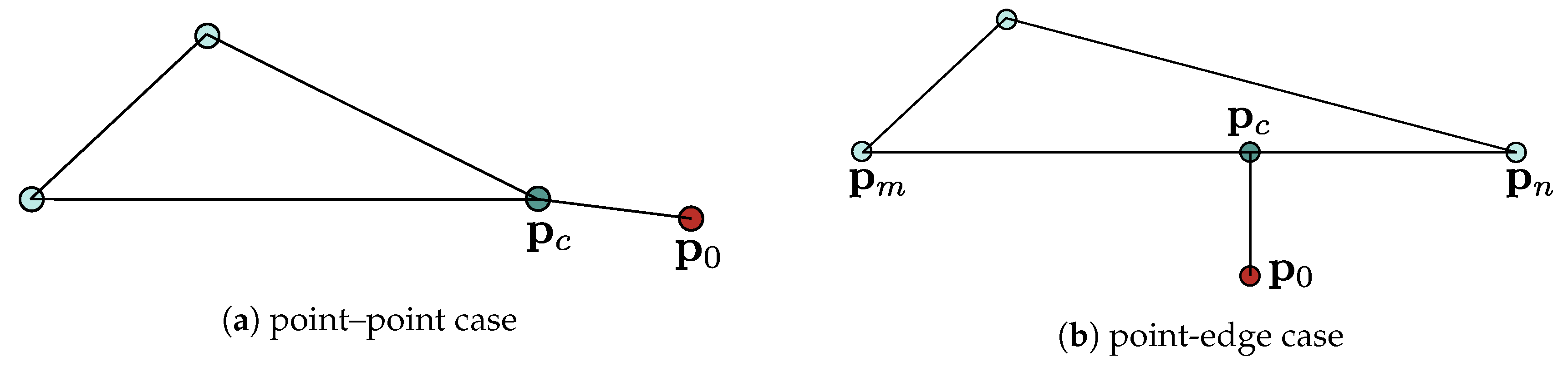
3. Point-Edge and Point-Point Cases

If the projection of ${\mathbf{p}}_0$ falls outside of the interior area of the triangle (Figure 2), the closest point ${\mathbf{p}}_c$ coincides with one of the vertices or belongs to one of the edges of the triangle. In the point–point case (Figure 3a), the squared distance is expressed as

$$s={\left|{\mathbf{p}}_0-{\mathbf{p}}_c\right|}^2,$$

where ${\mathbf{p}}_c$ is one of ${\mathbf{p}}_1,{\mathbf{p}}_2$ or ${\mathbf{p}}_3$. The derivatives of s with respect to $x_i$ are obtained trivially, and the details are not discussed here.

Figure 2. Partitioning of the plane by the triangle domain. Different domains are distinguished by the values of barycentric coordinates of the projection of ${\mathbf{p}}_0$ onto the plane of the triangle.

Figure 3. The closest point ${\mathbf{p}}_c$ may coincide with (a) one of triangle’s vertices or (b) belong to one of the edges.

In the point-edge case, one of the barycentric coordinates of ${\mathbf{p}}_c$ is zero, which simplifies Expression (2). Let ${\mathbf{p}}_m$ and ${\mathbf{p}}_n$ be the vertices of the edge, to which the closest point ${\mathbf{p}}_c$ belongs ( Figure 3b). Then ${\mathbf{p}}_c$ is expressed as the linear combination:

$${\mathbf{p}}_c=(1-{\zeta }_k){\mathbf{p}}_m+{\zeta }_k{\mathbf{p}}_n,$$

where ${\zeta }_k$ is the non-zero barycentric coordinate of ${\mathbf{p}}_c$. This coordinate can be found as [5]:

$${\zeta }_k=\frac{({\mathbf{p}}_m-{\mathbf{p}}_0)·({\mathbf{p}}_n-{\mathbf{p}}_m)}{{\left|{\mathbf{p}}_n-{\mathbf{p}}_m\right|}^2}.$$

(20)

Similarly to the previous derivations, Expression (20) can be differentiated to obtain the first and the second derivatives of the ${\zeta }_k$, which are then substituted into Expressions (3) and (11).

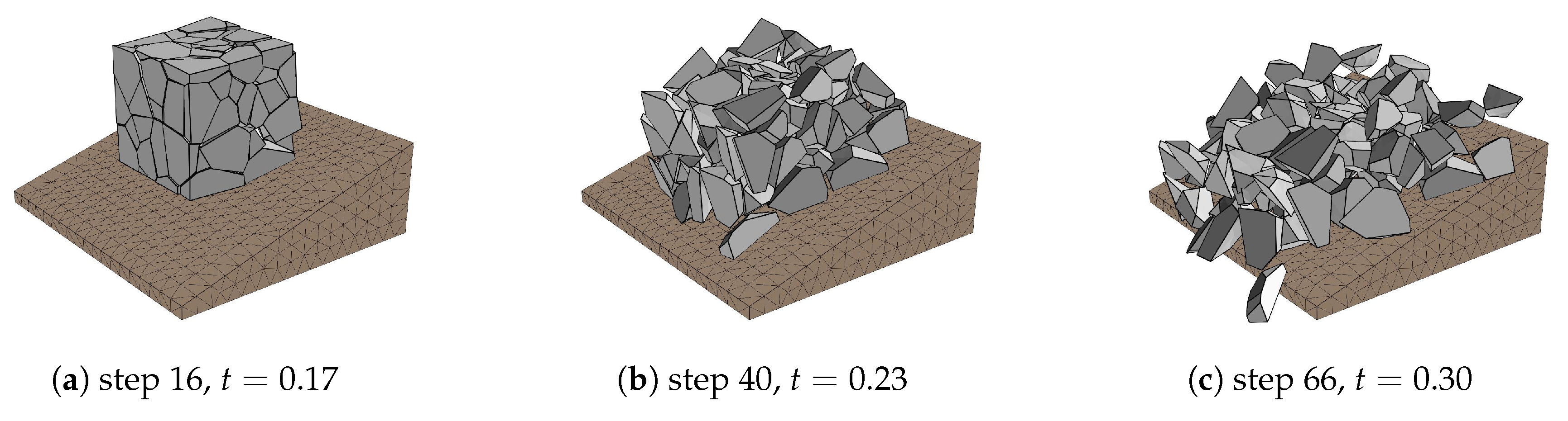
4. Algorithm and Testing

The calculations are implemented in double-precision floating-point arithmetic in C, and the tests are performed with squared distance s and its first and second derivatives. The first step is to determine the partition to which ${\mathbf{p}}_c$ belongs (Figure 2). This step coincides with the original point-triangle algorithm [1], but subsequent calculations are extended to evaluate $\frac{\partial s}{\partial x_i}$ and $\frac{{\partial }^{2}s}{\partial x_i\partial x_j}$. If ${\mathbf{p}}_c$ belongs to partitions 1, 3, 5, then the point-line algorithm is invoked. For partitions 2, 4, 6, point–point calculations are performed. For partition 0, the point-plane algorithm is used.

For testing, 10 million cases were generated, about $2/3$ of which are random coordinates that come from the uniform distribution in the range $[-1,1]$. The remaining cases come from the finite element simulation of fracture, where the point ${\mathbf{p}}_c$ is often close to one of the triangle’s vertices. Most of the cases that come from the simulation have a low ratio of the distance to the shortest edge of the triangle, in the range between ${10}^{-8}$ and ${10}^{-5}$. Such test cases result in a lower accuracy of the final answer than the random arrangements of points.

To evaluate the accuracy of the proposed algorithm, calculations are first performed using arbitrary precision arithmetic with at least 17 digits calculated precisely. These results are denoted $s_p,\frac{\partial s_p}{\partial x_i},\frac{{\partial }^2{s}_p}{\partial x_i\partial x_j}$ and are compared to the results obtained in floating-point arithmetic $s_c,\frac{\partial s_c}{\partial x_i},\frac{{\partial }^2{s}_c}{\partial x_i\partial x_j}$. Relative errors are computed separately for the squared distance, its first derivatives and its second derivatives:

$$E_0=\left|(s_c-s_p)/s_p\right|,$$

(21)

$$E_1=\underset{i}{max}\left|\left(\frac{\partial s_c}{\partial x_i}-\frac{\partial s_p}{\partial x_i}\right)/\frac{\partial s_p}{\partial x_i}\right|,$$

(22)

$$E_2=\underset{i,j}{max}\left|\left(\frac{{\partial }^2{s}_c}{\partial x_i\partial x_j}-\frac{{\partial }^2{s}_p}{\partial x_i\partial x_j}\right)/\frac{{\partial }^2{s}_p}{\partial x_i\partial x_j}\right|.$$

(23)

$E_0$ is the relative error of the squared distance and is used as a baseline to compare with the relative errors of the first and second derivatives $E_1$ and $E_2$. Ideally, the values of $E_0$, $E_1$ and $E_2$ would have the same order of magnitude. However, due to the large number of algebraic operations, the accuracy of the calculation of the second derivative is lower. The values $E_0$, $E_1$ and $E_2$ cover a wide range of values. In about half of the cases, the precision for calculating second derivatives is better than ${10}^{-13}$. However, the practical interest lies in investigating the worst cases because one incorrect calculation could affect a whole scientific study.

Discussion

The highest errors among all test cases are shown in Table 1. The values come from separate test cases: $E_{0_{max}}$ is the maximum error for s, $E_{1_{max}}$ is the maximum error for $\frac{\partial s_c}{\partial x_i}$ and $E_{2_{max}}$ is the maximum error for $\frac{{\partial }^2{s}_c}{\partial x_i\partial x_j}$. $E_{2_{max}}$ is higher than $E_{0_{max}}$ by two orders of magnitude, which is a good result, considering that it is the least accurate of 10 million tests. The tests show that the precision is adequate for all cases, including the ones form the collision simulation.

Table 1. Relative errors for squared distance and its first and second derivatives. The maximum values from 10 million test cases are shown.

Error Measure	Value
$E_{0_{max}}$	$3.78\times {10}^{-5}$
$E_{1_{max}}$	$2.75\times {10}^{-5}$
$E_{2_{max}}$	$1.27\times {10}^{-3}$

Cases with the lowest accuracy usually correspond to the variables whose absolute values are very small, and computer simulations are often robust against such cases. For example, results of the grain interaction simulation where the current algorithm is applied are shown on Figure 4. The simulation advances with large time steps even when multiple fragments interact with each other.

Figure 4. Simulation of falling and colliding grains performed with implicit finite element method.

The ratio between the distance and the largest edge of the triangle is one of the factors that affect the precision. When this ratio drops below ${10}^{-10}$, the accuracy of the result is likely to deteriorate. The problem of the round-off error is common in numerical analysis and should be addressed properly. If the influence of the round-off error is suspected when applying this algorithm, additional testing should be performed. In some cases, calculations can be performed with arbitrary-precision arithmetic to yield accurate results.

5. Conclusions

The presented algorithm has O(1) time and space complexity. Only static memory allocation takes place. The algorithm has several branches that evaluate algebraic expressions sequentially, with each branch completing in constant time. The main contribution of the authors is the derivation of the exact formulae for the gradient and the Hessian of the distance function. Additionally, testing of the reference implementation was performed to ensure that adequate precision is met. The proposed algorithm may be used in applications where point-triangle distance derivatives are required. The potential future work may include precision testing for more complex cases. The C code is available as open-source [6] and may be modified by the research community as needed.

References

- Eberly, D. Distance between Point and Triangle in 3D. 1999. Available online: https://www.geometrictools.com/Documentation/DistancePoint3Triangle3.pdf.pdf (accessed on 9 July 2018).
- Laursen, T.A. Computational Contact and Impact Mechanics: Fundamentals of Modeling Interfacial Phenomena in Nonlinear Finite Element Analysis; Springer Science & Business Media: Heidelberg/Berlin, Germany, 2013. [Google Scholar]
- Pfaff, T.; Narain, R.; De Joya, J.M.; O’Brien, J.F. Adaptive tearing and cracking of thin sheets. ACM Trans. Graph. 2014, 33, 110. [Google Scholar] [CrossRef]
- Fisher, S.; Lin, M.C. Fast penetration depth estimation for elastic bodies using deformed distance fields. In Proceedings of the Intelligent Robots and Systems, Maui, HI, USA, 29 October–3 November 2001; Volume 1, pp. 330–336. [Google Scholar]
- Weisstein, E.W. Point-Line Distance–3-Dimensional. MathWorld–A Wolfram Web Resource. Available online: http://mathworld.wolfram.com/Point-LineDistance3-Dimensional.html (accessed on 10 July 2018).
- Gribanov, I. Distance Derivatives, GitHub Repository. Available online: https://github.com/Spear520/dist/ (accessed on 10 July 2018).
© 2018 by the authors. Licensee MDPI, Basel, Switzerland. This article is an open access article distributed under the terms and conditions of the Creative Commons Attribution (CC BY) license (http://creativecommons.org/licenses/by/4.0/).