A Class of Algorithms for Continuous Wavelet Transform Based on the Circulant Matrix

Abstract

The Continuous Wavelet Transform (CWT) is an important mathematical tool in signal processing, which is a linear time-invariant operator with causality and stability for a fixed scale and real-life application. A novel and simple proof of the FFT-based fast method of linear convolution is presented by exploiting the structures of circulant matrix. After introducing Equivalent Condition of Time-domain and Frequency-domain Algorithms of CWT, a class of algorithms for continuous wavelet transform are proposed and analyzed in this paper, which can cover the algorithms in JLAB and WaveLab, as well as the other existing methods such as the $cwt$ function in the toolbox of MATLAB. In this framework, two theoretical issues for the computation of CWT are analyzed. Firstly, edge effect is easily handled by using Equivalent Condition of Time-domain and Frequency-domain Algorithms of CWT and higher precision is expected. Secondly, due to the fact that linear convolution expands the support of the signal, which parts of the linear convolution are just the coefficients of CWT is analyzed by exploring the relationship of the filters of Frequency-domain and Time-domain algorithms, and some generalizations are given. Numerical experiments are presented to further demonstrate our analyses.

1. Introduction

In recent years, different Time-frequency representations, such as, empirical mode decomposition [1], wavelet transform [2] and its variants, empirical wavelet transform [3,4], synchrosqueezed wavelet transforms [5], have been used for analyzing nonlinear and non-stationary signals. To name only a few, the method of fused empirical mode decomposition and wavelets is applied to detection-location of damage in a truss-type structure [6]; Wavelet transform is used for the pattern recognition for diagnosis, condition monitoring and fault detection [7,8,9]. It is also used to design an algorithm for Brain-computer interfacing [10], to detect the exact onset of chipping of the cutting tool from the workpiece profile [11], to determine the length of piles [12]; Synchrosqueezed wavelet transform is used for global and local health condition assessment of structures [13], for modal parameters identification of smart civil structures [14].

This paper gives priority to the computation of continuous wavelet transform (CWT) for Morlet-type wavelets. However, for this type of wavelets, it is not possible to use a multiresolution framework for the computation of CWT [15]. Michael Unser [16] used Exponentials or B-spline window to approximate Gabor window, which can achieve $\mathcal{O}\left(N\right)$ complexity per scale. Another kind of method for the computation of CWT with Morlet-type wavelets concerns directly discretizing the integral expression of Wavelet transform. These methods allow us to use arbitrary values for the scale variable, and require the explicit expression of wavelet function and cannot deal with those wavelets without analytic expressions such as Daubechies wavelets [17]. This kind of method include Time-domain methods [17] and Frequency-domain methods [18].

Frequency-domain methods for CWT are also widely used in the freewares such as JLAB (available online http://www.jmlilly.net), Wavelab (available online http://www-stat.stanford.edu/$\sim$wavelab), which can achieve satisfactory precision while the edge effect, defined in [18], may occur and the complexity of those methods is $\mathcal{O}(Nlog(N\left)\right)$ where N is the length of the signal.

The function $cwt$ in wavelet toolbox of MATLAB, which has poorer precision than Frequency-domain methods mentioned above, is a representation of the Time-domain method [17]. For the details of the comparison of the different methods, we refer to [17].

The computation of linear convolution can be realized by using the circular convolution, while the computation of circular convolution can be computed by using the FFT-based fast method [19]. In this paper, a novel and simple method is given to prove the FFT-based fast method of linear convolution by exploiting the structures of circulant matrix. After introducing Equivalent Condition of Time-domain and Frequency-domain Algorithms of CWT, a class of algorithms for continuous wavelet transform are proposed and analyzed, which can cover the algorithms in JLAB and WaveLab, as well as the other existing methods such as the $cwt$ function in the toolbox of MATLAB. In this framework, two theoretical issues for the computation of CWT are analyzed.

Firstly, by using Equivalent Condition of Time-domain and Frequency-domain Algorithms of CWT to design Frequency-domain Algorithm, the edge effect, defined in [18], can be avoided. To be specific, in [18], the time series is padded with sufficient zeroes to bring the total length N up to the next-higher power of two, thus limiting the edge effects and speeding up the Fourier transform. In fact, the same number of zeros is padded for all scales in [18], which may cause some troubles, for example, increasing the amount of data to process, and consequently the computational complexity. In this article, the time series (the data) is padded with $2aT$ zeros while a is the scale. These two zero padding methods are compared in Remark 2 of this paper.

Secondly, due to the fact that linear convolution expands the support of the signal, which parts of the linear convolution are just the coefficients of CWT is analyzed by exploring the relationship of the filters of Frequency-domain and Time-domain algorithms (see Theorem 4), and some generalizations are given (see Theorem 5).

This paper is organized as follows. Section 2 gives some definitions and theorems concerning circulant matrix and linear convolution. Section 3 analyzes algorithms of continuous wavelet transform. Section 4 presents numerical experiments to demonstrate our results and finally, we end this paper with conclusions and discussions in Section 5.

2. Primary Definitions and Theorems

Definition 1.

Circulant matrix: An $N\times N$ circulant matrix $\mathbf{C}$ takes the form [20,21]

$$\mathbf{C}=\left[\begin{array}{ccccc}{c}_0& c_{N-1}& \cdots & c_2& c_1\\ c_1& c_0& c_{N-1}& c_2\\ ⋮& c_1& c_0& \ddots & ⋮\\ c_{N-2}& \ddots & \ddots & c_{N-1}\\ c_{N-1}& c_{N-2}& \cdots & c_1& c_0\end{array}\right]$$

(1)

A circulant matrix is fully specified by one vector, c, which appears as the first column of $\mathbf{C}$.

Definition 2.

Discrete Fourier transform(DFT): The sequence of N complex numbers ${[x_0,x_1,\cdots ,x_{N-1}]}^{\mathrm{T}}$ is transformed into an N-periodic sequence of complex numbers [22]

$$X_k=\sum _{n=0}^{N-1}{x}_n{\omega }_k^{-n},k=0,1,\cdots ,N-1,$$

(2)

where $i=\sqrt{-1}$, ${\omega }_k=e^{\frac{2\pi ki}{N}}$ is the N-th root of unity.

Equation (2) can be written as

$$\left(\begin{array}{c}{X}_0\\ X_1\\ ⋮\\ X_{N-1}\end{array}\right)={\mathbf{F}}_{\mathbf{N}}\left(\begin{array}{c}{x}_0\\ x_1\\ ⋮\\ x_{N-1}\end{array}\right)$$

(3)

where ${\mathbf{F}}_{\mathbf{N}}$ is a $N\times N$ matrix, defined as

$${\mathbf{F}}_{\mathbf{N}}(k,j)={\omega }_{k-1}^{-(j-1)},k,j=1,2,\cdots ,N.$$

(4)

It is easy to verify that

$${{\mathbf{F}}_{\mathbf{N}}}^{-1}=\frac{1}{N}{{\mathbf{F}}_{\mathbf{N}}}^{\ast }$$

(5)

where “$\ast$” means conjugate transposition. Then, the inverse discrete Fourier transform (IDFT) is given as

$$\left(\begin{array}{c}{x}_0\\ x_1\\ ⋮\\ x_{N-1}\end{array}\right)=\frac{1}{N}{{\mathbf{F}}_{\mathbf{N}}}^{\ast }\left(\begin{array}{c}{X}_0\\ X_1\\ ⋮\\ X_{N-1}\end{array}\right)$$

(6)

Theorem 1.

References [20,21] The matrix $\mathbf{C}$ defined in (1) can be diagonalized by the DFT matrix ${\mathbf{F}}_{\mathbf{N}}$, namely,

$$\mathbf{C}={{\mathbf{F}}_{\mathbf{N}}}^{-1}diag\left({\mathbf{F}}_{\mathbf{N}}c\right){\mathbf{F}}_{\mathbf{N}}$$

(7)

where c is the first column of $\mathbf{C}$, i.e., $c={\left[\begin{array}{cccc}{c}_0& c_1& \cdots & c_{N-1}\end{array}\right]}^{\mathrm{T}}$.

Proof. 

It is easy to verify that the normalized eigenvectors of $\mathbf{C}$ are given by

$$v_j=\frac{1}{\sqrt{N}}{(1,{\omega }_j,{\omega }_j^2,\cdots ,{\omega }_j^{N-1})}^{\mathrm{T}},j=0,1,\cdots ,N-1,$$

(8)

where ${\omega }_j=e^{\frac{2\pi ij}{N}}$ with $i=\sqrt{-1}$ is the N-th root of unity. The corresponding eigenvalues are then given by

$$\begin{array}{ccc}\hfill {\lambda }_j& =& c_0+c_{N-1}{\omega }_j+c_{N-2}{\omega }_j^2+\cdots +c_1{\omega }_j^{N-1}\hfill \\ & =& c_0{\omega }_j^{-0}+c_{N-1}{\omega }_j^N{\omega }_j^{-(N-1)}+\hfill \\ & & c_{N-2}{\omega }_j^N{\omega }_j^{-(N-2)}+\cdots +c_1{\omega }_j^N{\omega }_j^{-1}\hfill \\ & =& \sum _{k=0}^{N-1}{c}_k{\omega }_j^{-k},j=0,1,\cdots ,N-1.\hfill \end{array}$$

(9)

From (2), (3) and (9), we have

$$\left(\begin{array}{c}{\lambda }_0\\ ⋮\\ {\lambda }_{N-1}\end{array}\right)={\mathbf{F}}_{\mathbf{N}}\left(\begin{array}{c}{c}_0\\ ⋮\\ c_{N-1}\end{array}\right)={\mathbf{F}}_{\mathbf{N}}c$$

(10)

Using ${\left\{v_j\right\}}_{j=0}^{N-1}$ defined in Equation (8) as column vectors to form a $N\times N$ matrix ${\mathbf{U}}_{\mathbf{N}}$

$${\mathbf{U}}_{\mathbf{N}}=[v_0,v_1,\cdots ,v_{N-1}],$$

(11)

then we have

$$\mathbf{C}={\mathbf{U}}_{\mathbf{N}}\left(\begin{array}{ccc}{\lambda }_0& & \\ & \ddots & \\ & & {\lambda }_{N-1}\end{array}\right){{\mathbf{U}}_{\mathbf{N}}}^{\ast }.$$

(12)

Furthermore, we have ${{\mathbf{U}}_{\mathbf{N}}}^{\ast }=\frac{1}{\sqrt{N}}{\mathbf{F}}_{\mathbf{N}},{\mathbf{U}}_{\mathbf{N}}=\sqrt{N}{{\mathbf{F}}_{\mathbf{N}}}^{-1}$ from (4), (5) and (11). Then we have

$$\mathbf{C}={{\mathbf{F}}_{\mathbf{N}}}^{-1}diag\left({\mathbf{F}}_{\mathbf{N}}c\right){\mathbf{F}}_{\mathbf{N}}$$

(13)

 ☐

Definition 3.

Linear convolution [23]: A time-invariant linear operator L can be represented as a linear convolution. To be specific, we denote by $\delta \left[n\right]$ the discrete Dirac

$$\delta \left[n\right]=\left\{\begin{array}{cc}1\hfill & ifn=0\hfill \\ 0\hfill & ifn\ne 0\hfill \end{array}\right..$$

Any signal $f\left[n\right]$ can be decomposed as a sum of shifted Diracs:

$$f\left[n\right]=\sum _{p=-\infty }^{+\infty }f\left[p\right]\delta [n-p].$$

Let $L\delta \left[n\right]=h\left[n\right]$ be the discrete impulse response. Linearity and time invariance implies that

$$g\left[n\right]=Lf\left[n\right]=\sum _{p=-\infty }^{\infty }f\left[p\right]h[n-p]:\stackrel{\mathrm{def}}{=}f★h\left[n\right],$$

(14)

where “$★$” represents linear convolution.

Definition 4.

Causality and Stability [23]: A discrete filter L is causal if $Lf\left[p\right]$ depends only on the values of $f\left[n\right]$ for $n\le p$. The convolution formula (14) implies that $h\left[n\right]=0$ if $n<0$.

A discrete filter L is stable if any bounded input signal $f\left[n\right]$ produces a bounded output signal $Lf\left[n\right]$. One can verify that the filter is stable if and only if $h\in l^1\left(\mathbb{Z}\right)$.

Proposition 1.

Assume that the length of f and h are finite. To be specific, If $f={[f_0,f_1,\cdots ,f_{n-\beta -1}]}^{\mathrm{T}}$, and $h={[h_0,h_1,\cdots ,h_{\beta }]}^{\mathrm{T}}$, then the linear convolution of f and h defined in (14) can be written as

$$g=f★h=\mathbf{H}f$$

(15)

where $\mathbf{H}\in R^{n\times (n-\beta )}$, and

$$\mathbf{H}=\left[\begin{array}{ccccc}{h}_0& & & & \\ h_1& h_0& & & \\ ⋮& & \ddots & & \\ h_{\beta }& & & \ddots & \\ & \ddots & & & h_0\\ & & \ddots & & h_1\\ & & & \ddots & ⋮\\ & & & & h_{\beta }\end{array}\right].$$

(16)

Proof. 

We refer the reader to [19] for details. ☐

Suppose we wish to compute the polynomial product $c\left(x\right)=a\left(x\right)·b\left(x\right)$, the ordinary product expression for the coefficients of $c\left(x\right)$ involves a linear convolution.

Definition 5.

Circular convolution [19]: The circular convolution of a signal ${\left\{x\left[k\right]\right\}}_{k=0}^{N-1}$ with a signal ${\left\{c\left[k\right]\right\}}_{k=0}^{N-1}$ is defined as a matrix vector multiplication as follows.

$$y:\stackrel{\mathrm{def}}{=}x⊛c=\mathbf{C}·\left[\begin{array}{c}x\left[0\right]\\ x\left[1\right]\\ ⋮\\ x[N-1]\end{array}\right]$$

(17)

where $\mathbf{C}$ is defined in Equation (1), and “$⊛$” represents circular convolution.

Proposition 2.

The computation of circular convolution can be realized by using FFT-based fast method. In other word, Equation (17) can be written as

$$y={{\mathbf{F}}_{\mathbf{N}}}^{-1}diag\left({\mathbf{F}}_{\mathbf{N}}c\right){\mathbf{F}}_{\mathbf{N}}x.$$

(18)

Proof. 

The matrix involved in (17) is a circulant matrix, thus (18) is obtained by using Theorem 1. ☐

The equivalent condition of circular convolution and linear convolution will be given in the following theorem.

Theorem 2.

Assume $f={[f_0,f_1,\cdots ,f_{n-\beta -1}]}^{\mathrm{T}}$, $h={[h_0,h_1,\cdots ,h_{\beta }]}^{\mathrm{T}}$, $\tilde{f}={[f_0,f_1,\cdots ,f_{n-\beta -1},\stackrel{\beta }{\underbrace{0,\cdots ,0}}]}^{\mathrm{T}}$, $\tilde{h}={[h_0,h_1,\cdots ,h_{\beta },\stackrel{n-\beta -1}{\underbrace{0,\cdots ,0}}]}^{\mathrm{T}}$, then linear convolution $g=f★h$ of f and h defined in (14) can be computed as circular convolution $\tilde{f}⊛\tilde{h}$ of $\tilde{f}$ and $\tilde{h}$, namely,

$$g=f★h=\tilde{f}⊛\tilde{h}={{\mathbf{F}}_{\mathbf{N}}}^{-1}({\mathbf{F}}_{\mathbf{N}}\tilde{h}.\ast {\mathbf{F}}_{\mathbf{N}}\tilde{f}).$$

(19)

where ${\mathbf{F}}_{\mathbf{N}}$, ${{\mathbf{F}}_{\mathbf{N}}}^{-1}$ are defined by (4), (5) respectively; “$.\ast$”means componentwise product of two vectors.

Proof. 

From Proposition (1), we get $g=\mathbf{H}f$ , where $\mathbf{H}\in R^{n\times (n-\beta )}$ is defined in (16). Now extend $\mathbf{H}$ to a circulant matrix [21]

$$\mathbf{C}=[\mathbf{H},\widehat{\mathbf{H}}]=\left[\begin{array}{cccccccc}{h}_0& & & & & h_{\beta }& & h_1\\ h_1& h_0& & & & & \ddots & ⋮\\ ⋮& & \ddots & & & & & h_{\beta }\\ h_{\beta }& & & \ddots & & & & \\ & \ddots & & & h_0& & & \\ & & \ddots & & h_1& h_0& & \\ & & & \ddots & ⋮& ⋮& \ddots & \\ & & & & h_{\beta }& h_{\beta -1}& \cdots & h_0\end{array}\right],$$

(20)

thus the first column of $\mathbf{C}$ is $\tilde{h}$. Therefore,

$$g=\mathbf{H}f=[\mathbf{H},\widehat{\mathbf{H}}]\tilde{f}=\mathbf{C}\tilde{f}=\tilde{f}⊛\tilde{h}={\mathbf{F}}_{{\mathbf{N}}^{-1}}({\mathbf{F}}_{\mathbf{N}}\tilde{h}.\ast {\mathbf{F}}_{\mathbf{N}}\tilde{f})$$

by using Definition 5 and Proposition 2. ☐

From Theorem 2, the algorithm of linear convolution of $g=f★h$ is given as follows (See Algorithm 1).

Algorithm 1: FFT-based fast method for linear convolution.

Input:  the signal, $f\left[k\right],k=0,1,\cdots ,n-\beta -1$  the signal, $h\left[k\right],k=0,1,\cdots ,\beta$  Output:  the linear convolution of f and h, $g\left[k\right],k=0,1,\cdots ,n-1$  1. Set $n=length\left(f\right)+length\left(h\right)-1;$  2. Appending an array of zeros to the end of h to obtain $\tilde{h}$ so that the length of $\tilde{h}$ is n.  3. Appending an array of zeros to the end of f to obtain $\tilde{f}$ so that the length of $\tilde{f}$ is n  4. $g=ifft(fft(\tilde{h}).\ast fft(\tilde{f}))$

Additionally, the asymptotic time complexity is $\mathcal{O}\left(nlo{g}_2\left(n\right)\right)$ for Algorithm 1. Note the condition $n=length\left(f\right)+length\left(h\right)-1$ plays a pivotal role in the equivalence of linear convolution and circular convolution. This condition will also be used in the following part of this paper.

Definition 6.

Equivalent Condition of Linear Convolution and Circular Convolution: Let $f,h,\tilde{f},\tilde{h}$ be defined in Theorem 2. The condition $length(\tilde{h})=length(\tilde{f})=length(f)+length(h)-1$ is called Equivalent Condition of Linear Convolution and Circular Convolution.

3. A Class of Algorithms for Continuous Wavelet Transform

3.1. Time-Domain Algorithm for CWT

Definition 7.

Continuous wavelet transform: The continuous wavelet transform of a function $f\left(t\right)$ at a scale $a\in R^{+}$ and translational value $b\in R$ is expressed by the following integral [17]

$$W_f(a,b):\stackrel{\mathrm{def}}{=}{\int }_{-\infty }^{+\infty }f\left(t\right)\frac{1}{a}\overline{\psi }(\frac{t-b}{a})\mathrm{d}t$$

(21)

where $\psi \left(t\right)$ is a continuous function called the mother wavelet and the overline represents the operation of complex conjugate.

For real-life applications, the length of $f\left(t\right)$ is finite and the support of $\psi \left(t\right)$ is compact. Without loss of generality, assume the sampling rates of the signal and the wavelet are equal to 1, then Equation (21) can be written as

$$W_f^a[m]=\sum _{k=-\infty }^{+\infty }f(k)\frac{1}{a}\overline{\psi }(\frac{k-m}{a}),wherem\in \mathbb{Z}.$$

(22)

Assume the sampled signal is ${\left\{f\left[i\right]\right\}}_{i=0}^{N-1}$ and the support of the mother wavelet $\psi \left(t\right)$ is $[-T,T]$. If define

$${\tilde{\psi }}_a(t):\stackrel{\mathrm{def}}{=}\frac{1}{a}\overline{\psi }(\frac{aT-t}{a})$$

(23)

then the support of ${\tilde{\psi }}_a\left(t\right)$ is $[0,2aT]$. Now, we can get the following result.

Theorem 3.

Assume the length of $f\left(t\right)$ is finite and the support of $\psi \left(t\right)$ is compact, and the sampling rates of the signal and the wavelet are equal to 1, then CWT of ${\left\{f\left[i\right]\right\}}_{i=0}^{N-1}$ can be written as

$$\begin{array}{c}\hfill W_f^a\left[m\right]=\sum _{k=0}^{N-1}f\left(k\right){\tilde{\psi }}_a(m+aT-k)=f★{\tilde{\psi }}_a[m+aT],wherem=0,1,\cdots ,N-1,\end{array}$$

(24)

where we assume $aT$ is an integer for the convenience of analysis. Furthermore, the corresponding filter is causal and stable.

Proof. 

By using Proposition 1 and Equations (23) and (24) is deduced from (22). Furthermore, define

$$h_a\left[i\right]={\tilde{\psi }}_a\left(i\right),i\in \mathbb{Z}$$

(25)

then the discrete filter ${\left\{h_a\left[i\right]\right\}}_{i\in \mathbb{Z}}$ is causal and stable since $h_a\left[i\right]={\tilde{\psi }}_a\left(i\right)=0$ if $i<0$ and $h_a\in l^2\left(\mathbb{Z}\right)$. Furthermore, Equation (24) can be written as

$$W_f^a\left[m\right]=f★h_a[m+aT],wherem=0,1,\cdots ,N-1.$$

(26)

 ☐

In brief, ${\{W_f^a\left[i\right]\}}_{i=0}^{N-1}$ are just the ${\{f★h_a\left[i\right]\}}_{i=aT}^{aT+N-1}$ while ${\{f★h_a\left[i\right]\}}_{i=0}^{2aT+N-1}$ can be implemented with linear convolution [17]. From Algorithm 1, we can get the algorithm of CWT (see Algorithm 2).

Algorithm 2: Time-domain fast algorithm for CWT.

Input:  the signal, $f\left[n\right],n=0,1,\cdots ,N-1$  mother wavelet, $\psi \left(t\right)$  scale, a  T, where $[-T,T]$ is the support of $\psi \left(t\right)$.  Output:wavelet coefficients, $W_f^a\left[i\right],i=0,1,\cdots ,N-1$  1. Let $\tilde{f}={[f_0,f_1,\cdots ,f_{N-1},\stackrel{2aT}{\underbrace{0,\cdots ,0}}]}^{\mathrm{T}};$  2. Let ${\tilde{\psi }}_a(t)=\frac{1}{a}\overline{\psi }(\frac{aT-t}{a})$, where the overline represents the operation of complex conjugate;  3. Let $h_a[n]={\tilde{\psi }}_a(n),n=0,1,\cdots ,2aT$;  4. Let ${\tilde{h}}_a={[h_a[0],h_a[1],\cdots ,h_a[2aT],\stackrel{N-1}{\underbrace{0,\cdots ,0}}]}^{\mathrm{T}};$  5. $te{m}_a[i]=ifft(fft(\tilde{f}).\ast fft({\tilde{h}}_a)),i=0,1,\cdots ,2aT+N-1$;  6. $W_f^a[i]=te{m}_a[aT+i],i=0,1,\cdots ,N-1$.

3.2. Frequency-Domain Algorithm for CWT

The algorithm can be further optimized by taking advantage of the analytic expression of $\widehat{\psi }\left(\omega \right)$, the Fourier transform of the mother wavelet $\psi \left(t\right)$. In fact, the wavelet transform defined in (21) can also be written as a frequency integration by applying the Fourier Parseval formula [23].

$$W_f(a,b)=\frac{1}{2\pi }{\int }_{-\infty }^{+\infty }\widehat{f}\left(\omega \right)\overline{\widehat{\psi }}\left(a\omega \right)e^{ib\omega }\mathrm{d}\omega$$

(27)

Assume the sampled signal is ${\left\{f\left[n\right]\right\}}_{n=0}^{N-1}$. Discretizing (27) and considering the periodic property of discrete Fourier transform yields

$$\begin{array}{ccc}\hfill W_f^a[n]& =& \frac{1}{M}\sum _{k=-\frac{M}{2}+1}^{\frac{M}{2}}\widehat{f}(\frac{2\pi }{M}k)\overline{\widehat{\psi }}(\frac{2\pi }{M}ka)e^{i\frac{2\pi }{M}kn}\hfill \\ & =& \frac{1}{M}\sum _{k=0}^{M-1}\widehat{f}(\frac{2\pi }{M}k)\overline{\widehat{\psi }}(\frac{2\pi }{M}ka)e^{i\frac{2\pi }{M}kn},\hfill \\ & where& n=0,1,\cdots ,M-1.\hfill \end{array}$$

(28)

It is seen by comparing (28) and (18) that (28) represents a circular convolution. By considering Equivalent Condition of Linear Convolution and Circular Convolution, It is reasonable to let

$$M=2aT+N.$$

(29)

In this case, the values of ${\{\widehat{f}(\frac{2\pi }{M}k)\}}_{k=0}^{M-1}$ can be computed as the discrete Fourier transform of $\tilde{f}={[f_0,f_1,\cdots ,f_{N-1},\stackrel{M-N}{\underbrace{0,\cdots ,0}}]}^{\mathrm{T}}$. As for the computation of ${\{\overline{\widehat{\psi }}(\frac{2\pi }{M}ka)\}}_{k=0}^{M-1}$, we can make use of the analytic expression of $\widehat{\psi }(\omega )$. For example, the Morlet wavelet is defined as [24]

$$\psi \left(t\right):\stackrel{\mathrm{def}}{=}\sqrt{\frac{2}{\pi {\sigma }^2}}{e}^{-\frac{t^2}{2{\sigma }^2}}{e}^{i\eta t},$$

(30)

then

$$\overline{\widehat{\psi }}\left(\omega \right)=\widehat{\psi }\left(\omega \right)=2e^{-\frac{{\sigma }^2{(\omega -\eta )}^2}{2}},$$

(31)

where ${\sigma }^2$ is shape parameter, and $\eta$ is center frequency. Furthermore, the Morlet wavelet is approximately analytic and therefore $\overline{\widehat{\psi }}\left(\frac{2\pi }{M}ka\right)\approx 0$ for $k<0$. So

$$\overline{\widehat{\psi }}(\frac{2\pi }{M}ka)\approx 0,fork>\frac{M}{2},$$

(32)

by the periodic property of discrete Fourier transform. Equation (32) will be used to design algorithm of CWT (see the 4th–6th steps of Algorithms 3).

Definition 8.

Equivalent Condition of Time-domain and Frequency-domain Algorithms of CWT: $M=2aT+N$ in Equation (29) is called Equivalent Condition of Time-domain and Frequency-domain Algorithms of CWT.

Remark 1.

In freeware such as Wavelab, the parameter M in Equation (29) takes value N, where N is the length of signal. In this case, ${\{\widehat{f}(\frac{2\pi }{M}k)\}}_{k=0}^{M-1}$ can be obtained as the discrete Fourier transform of the data. Furthermore, the length of the result of $\mathbf{ifft}$ is just N. However, the method will produce artificial periodicity, which is called edge effect by Torrence [18], in the wavelet coefficients if signal is not periodic. In order to limit the edge effect, in [18], the data is padded with sufficient zeros before doing the CWT, then the first N coefficients of the corresponding convolution are just the coefficients of the CWT. Nevertheless, the reason for this is not answered in previous papers in the author’s knowledge. Put another way. Why the last step of Algorithm 3 is dissimilar from the last step of Algorithm 2? The answer will be given in the following Theorem 4.

Lemma 1.

The filter used in Equation (27) is

$${\tilde{\tilde{\psi }}}_a(t)=\frac{1}{a}\overline{\psi }(\frac{-t}{a}).$$

(33)

Proof. 

We refer the reader to [23] for details. ☐

Theorem 4.

The wavelet coefficients of the CWT of ${\left\{f\left[n\right]\right\}}_{n=0}^{N-1}$ is the first N coefficients of (28). While the length of the total coefficients of (28) is M.

Proof. 

The filter used in Theorem 3 is ${\tilde{\psi }}_a$ defined in (23); therefore, ${\tilde{\tilde{\psi }}}_a(t-aT)={\tilde{\psi }}_a\left(t\right)$. Define $L{\tilde{\psi }}_a=f★{\tilde{\psi }}_a$, then $L{\tilde{\tilde{\psi }}}_a=f★{\tilde{\tilde{\psi }}}_a$. Denote $\tilde{\tilde{\psi }}={\tilde{\tilde{\psi }}}_a$, $\tilde{\psi }={\tilde{\psi }}_a$, ${\tilde{\tilde{\psi }}}_{aT}=\tilde{\tilde{\psi }}(t-aT)=\tilde{\psi }$ for the simplicity of notation for this moment. By the property of time-invariant of L,

$$L\tilde{\psi }\left[n\right]=L{\tilde{\tilde{\psi }}}_{aT}\left[n\right]=L\tilde{\tilde{\psi }}[n-aT];$$

therefore

$$L\tilde{\psi }[n+aT]=L\tilde{\tilde{\psi }}\left[n\right].$$

That is to say

$${\{L{\tilde{\psi }}_a[n+aT]\}}_{n=0}^{N-1}={\{L{\tilde{\tilde{\psi }}}_a[n]\}}_{n=0}^{N-1}.$$

From Theorem 3, ${\{L{\tilde{\psi }}_a[n+aT]\}}_{n=0}^{N-1}$ is the wanted wavelet coefficients; therefore ${\{L{\tilde{\tilde{\psi }}}_a[n]\}}_{n=0}^{N-1}={\{f★{\tilde{\tilde{\psi }}}_a[n]\}}_{n=0}^{N-1}$ is the wanted wavelet coefficients. ☐

Theorem 5.

Assume that (Without loss of generality, $aT$ is assumed to be an integer.)

$$\begin{array}{ccc}\hfill L_m\left[n\right]& =& \frac{1}{M}\sum _{k=0}^{M-1}\widehat{f}(\frac{2\pi }{M}k)\overline{\widehat{\psi }}(\frac{2\pi }{M}ka)e^{-i\frac{2\pi }{M}kmaT}{e}^{i\frac{2\pi }{M}kn},\hfill \\ & & n=0,1,\cdots ,M-1;m=0,1,2,\hfill \end{array}$$

(34)

then

$${\{W_f^a\left[n\right]\}}_{n=0}^{N-1}={\left\{L_0\left[n\right]\right\}}_{n=0}^{N-1}={\left\{L_1\left[n\right]\right\}}_{n=aT}^{aT+N-1}={\left\{L_2\left[n\right]\right\}}_{n=M-N}^{M-1}.$$

Proof. 

If $m=0$, Equation (34) is simply Equation (28), the conclusion is deduced from Theorem 4.

Since

$$\begin{array}{ccc}\hfill F[{\tilde{\psi }}_a]\left(\omega \right)& =& {\int }_{-\infty }^{+\infty }\frac{1}{a}\overline{\psi }(\frac{aT-t}{a})e^{-it\omega }\mathrm{d}t\hfill \\ & =& e^{-iaT\omega }\overline{\widehat{\psi }}(a\omega ),\hfill \end{array}$$

(35)

thus $L_1\left[n\right]=f★{\tilde{\psi }}_a$, the conclusion is deduced from Theorem 3. If define ${\psi }_a^{\left(3\right)}=\frac{1}{a}\overline{\psi }(\frac{2aT-t}{a})$, the conclusion for the $m=2$ case can also be proved in the same way. ☐

Now, Frequency-domain algorithm of CWT with Morlet wavelet as the mother wavelet is given as follows.

Algorithm 3: Frequency-domain fast algorithm for CWT (In real application, the case $m=0$ is enough for the calculation of CWT).

Input:  the signal, $f[n],n=0,1,\cdots ,N-1$  scale, a  $\widehat{\psi }(\omega )$, the Fourier transform of the Morlet wavelet $\psi (t)$  T, where $[-T,T]$ is the support of $\psi (t)$.  Output:  wavelet coefficients, $W_f^a[i],i=0,1,\cdots ,N-1$  1. Let $\tilde{f}={[f_0,f_1,\cdots ,f_{N-1},\stackrel{2aT}{\underbrace{0,\cdots ,0}}]}^{\mathrm{T}};$  2. Define ${\phi }_m(\omega )=e^{-imaT\omega }\overline{\widehat{\psi }}(a\omega ),m=0,1,2$, where the overline represents the operation of    complex conjugate;  3. Let $M=2aT+N$;  4. If M is even, Let ${\widehat{\tilde{h}}}_a={[{\phi }_m(\frac{2\pi }{M}·0),{\phi }_m(\frac{2\pi }{M}·1),\cdots ,{\phi }_m(\frac{2\pi }{M}·\frac{M}{2}),\stackrel{\frac{M}{2}-1}{\underbrace{0,\cdots ,0}}]}^{\mathrm{T}};$  5. else ${\widehat{\tilde{h}}}_a={[{\phi }_m(\frac{2\pi }{M}·0),{\phi }_m(\frac{2\pi }{M}·1),\cdots ,{\phi }_m(\frac{2\pi }{M}·\frac{M-1}{2}),\stackrel{\frac{M-1}{2}}{\underbrace{0,\cdots ,0}}]}^{\mathrm{T}};$  6. end if  7. $te{m}_a[i]=ifft(fft(\tilde{f}).\ast ({\widehat{\tilde{h}}}_a)),i=0,1,\cdots ,2aT+N-1$;  8. switch(m)               case 0      $W_f^a[i]=te{m}_a[i],i=0,1,\cdots ,N-1$;               case 1      $W_f^a[i]=te{m}_a[i+aT],i=0,1,\cdots ,N-1$;               case 2      $W_f^a[i]=te{m}_a[i+2aT],i=0,1,\cdots ,N-1$.

Remark 2.

Note that the previous data preparation method takes $M=2^q$, where $q={min}_{n\in Z}\{2^n>N\}$ [17,18]. However, this method may fail for some real life data. We propose $M=N+2aT$, Equivalent Condition of Time-domain and Frequency-domain Algorithms of CWT, then the edge effect, defined in [18], that may occur in JLAB, Wavelab and [25] can be avoided. See Figures 6 and 7 for details.

4. Numerical Experiments

The experiments are conducted on two types of data, one for synthetic data, another for real-life data. Entropy can be used to measure the sparsity of wavelet coefficients [17]. In order to define entropy, $\left\{\right|W_f(a_i,b_j){{|}^2\}}_{i,j}$ are rearranged as ${\left\{c_k\right\}}_{k=1,\dots ,M}$, then are normalized to obtain:

$$d_k=\frac{c_k}{{\sum }_{k=1}^M{c}_k}.$$

(36)

The wavelet entropy is calculated as

$$Entropy=-\sum _{k=1}^M{d}_{k}log{d}_k,$$

(37)

with the convention $0log0=0$ by definition.

Experiments for Data 1: Data 1 is a synthetic signal with length N. The first half contains sinusoidal signal superimposition with three different frequencies, namely $a_{4}sin\left(30\pi t\right)+a_{3}sin\left(60\pi t\right)+a_{1}sin\left(120\pi t\right)$; The latter half contains the 60 Hz sinusoidal signal with amplitude $a_2$, namely $a_{2}sin\left(120\pi t\right)$, where $a_4=1,a_3=1.2,a_1=1.4,a_2=0.6$, and the sampling frequency is 400 Hz. Data 1 with length $N=1024$ is presented in Figure 1a. Figure 1b, the absolute values of CWT coefficients of Figure 1a, computed with the $awt$ function in Wavelab, where the shape parameter ${\sigma }^2=1$ and the center frequency $\eta =8$, manifests edge effects. Figure 1c without edge effects is computed by using the case 0 of Algorithm 3.

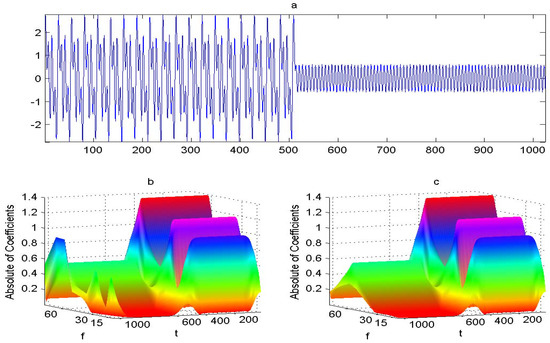
Figure 1. (a) is Data 1 with $N=1024$. (b) the absolute values of CWT coefficients of (a), computed with the $awt$ function in Wavelab, where the shape parameter ${\sigma }^2=1$ and the center frequency $\eta =8$, manifests edge effects. (c) without edge effects is computed with Algorithm 3.

Table 1 gives the computational results of Data 1 with wavelet parameter ${\sigma }^2=1,\eta =8$ by using different methods. “$cwt$” means the $cwt$ function in wavelet toolbox of Matlab. “Zhao’s method” is an improved version of $cwt$ [26]. ”Direct” means the computation method of linear convolution by using Equation (15). If the length of signal is far larger than the length of the filter, an “Overlap-add” procedure for the calculation of linear convolution is faster than Direct method and Algorithm 1 [23]. The “wavelet entropy” shown in Table 1 can measure the sparsity of wavelet coefficients [17]. “Err_i” means the relative error of $a_i$ and the corresponding maximum amplitude of CWT coefficients.

Table 1. Comparisons between the different CWT methods for Data 1.

Algorithm	N	CPU	Entropy	${\mathit{Err}}_1$	${\mathit{Err}}_2$	${\mathit{Err}}_3$	${\mathit{Err}}_4$
cwt	1024	0.2468	8.7125	$3.3605\times {10}^{-2}$	$3.5635\times {10}^{-2}$	−$1.4622\times {10}^{-2}$	−$4.0837\times {10}^{-2}$
	2048	0.2560	9.3815	$3.3605\times {10}^{-2}$	$3.5635\times {10}^{-2}$	−$1.4622\times {10}^{-2}$	−$4.0837\times {10}^{-2}$
Zhao’s	1024	0.0495	8.7068	−$1.0144\times {10}^{-2}$	$3.6888\times {10}^{-3}$	−$1.6761\times {10}^{-2}$	−$2.8041\times {10}^{-2}$
	2048	0.0562	9.3762	−$1.0144\times {10}^{-2}$	$3.6888\times {10}^{-3}$	−$1.6755\times {10}^{-2}$	−$2.8041\times {10}^{-2}$
Direct	1024	0.4724	8.7097	−$2.0333\times {10}^{-4}$	−$1.8504\times {10}^{-15}$	−$1.9882\times {10}^{-4}$	$4.9072\times {10}^{-14}$
	2048	0.8697	9.3784	−$2.0333\times {10}^{-4}$	−$7.0314\times {10}^{-15}$	−$1.9767\times {10}^{-4}$	−$9.6064\times {10}^{-11}$
Overlap-Add	1024	0.0291	8.7083	−$2.0333\times {10}^{-4}$	−$1.8504\times {10}^{-15}$	−$1.9882\times {10}^{-4}$	$4.8517\times {10}^{-14}$
	2048	0.0359	9.3777	−$2.0333\times {10}^{-4}$	−$6.4763\times {10}^{-15}$	−$1.9767\times {10}^{-4}$	−$9.6065\times {10}^{-11}$
Algorithm 2	1024	0.0204	8.7083	−$2.0333\times {10}^{-4}$	−$1.8504\times {10}^{-15}$	−$1.9882\times {10}^{-4}$	$4.8517\times {10}^{-14}$
	2048	0.0291	9.3777	−$2.0333\times {10}^{-4}$	−$6.4763\times {10}^{-15}$	−$1.9767\times {10}^{-4}$	−$9.6065\times {10}^{-11}$
Algorithm 3	1024	0.0155	8.7083	−$2.0333\times {10}^{-4}$	−$2.4055\times {10}^{-15}$	−$1.9882\times {10}^{-4}$	$4.7851\times {10}^{-14}$
	2048	0.0223	9.3777	−$2.0333\times {10}^{-4}$	−$7.0314\times {10}^{-15}$	−$1.9767\times {10}^{-4}$	−$9.6065\times {10}^{-11}$

From Table 1, we know that the precision, wavelet entropy of “Direct”, Algorithms 2 and 3, “Overlap-add” are almost the same and are more optimal to $cwt$ function in toolbox of Matlab. In fact, the precision of two methods in [17], “FFT based method” and the proposed method is almost the same. This phenomenon indicates some equivalence of these two methods. As a matter of fact, these two methods can be categorized as Algorithms 2 and 3 respectively.

Figure 2 is computed by using the case 1 of Algorithm 3. The wavelet coefficients of Figure 2b can exactly characterize the time-frequency local properties of data of Figure 1a. At the same time, Figure 2a,c fail to do so. In fact, it is known from the case 1 of Algorithm 3, the wavelet coefficients should be chosen as the middle part of the coefficients of the convolution. However, the wavelet coefficients of Figure 2a,c are respectively chosen as the first N and the last N part of the coefficients of the convolution.

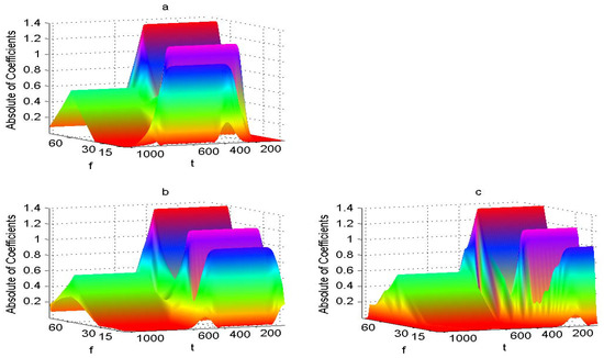
Figure 2. Figure 2 is computed by using the case 1 of Algorithm 3. The wavelet coefficients of (b) can exactly characterize the time-frequency local properties of data of (a). At the same time, (a,c) fail to do so.

Experiments for Data 2: Data 2 is the annual average temperature from 1 January 1951 to 31 December 2010 for No. 50978 weather station, Heilongjiang, China. Figure 3, Figure 4 and Figure 5, computed with different methods of CWT, namely, Algorithm 2, Zhao’s method, $cwt$ function in wavelet toolbox of Matlab, are the contours of the real part of coefficients of CWT for Data 2. The Morlet wavelet parameters are ${\sigma }^2=1,\eta =5$. The coefficients with negative values are plotted with a dotted, blue line, while the coefficients with positive values are plotted with a dashed, red line. It is obvious from these figures that the precision of Algorithm 2 is superior to that of Zhao’s method and $cwt$ function of Matlab.

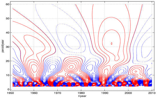
Figure 3. This contour is computed by using Algorithm 2 with the Morlet wavelet parameter ${\sigma }^2=1,\eta =5$ for Data 2.

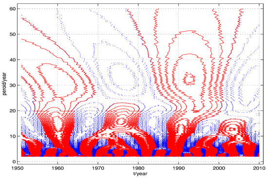
Figure 4. This contour is computed by using Zhao’s method with the Morlet wavelet parameter ${\sigma }^2=1,\eta =5$ for Data 2.

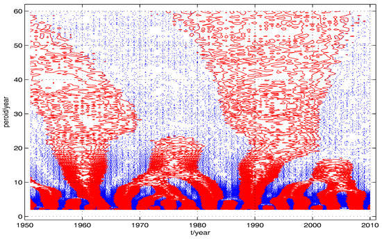
Figure 5. This contour is computed by using $CWT$ function in wavelet toolbox of Matlab with the Morlet wavelet parameter ${\sigma }^2=1,\eta =5$ for Data 2.

It is seen from Table 2 that the wavelet entropy for Algorithm 2 is the smallest of all the methods. Therefore, Algorithm 2 is the most suitable method for this temperature data.

Table 2. The wavelet entropy corresponding to different wavelet transform methods.

${\mathit{\sigma }}_2$	$\mathit{\eta }$	CWT	Zhao’s Method	Algorithm 2	Algorithm 3
1	5	9.5190	9.4150	9.4144	9.4534
1	6	9.5051	9.4044	9.4042	9.4332
1	7	9.4869	9.3897	9.3893	9.4117
1	8	9.4677	9.3713	9.3709	9.3892
1.5	5	9.5012	9.4030	9.4026	9.4304
1.5	6	9.4797	9.3832	9.3831	9.4037
1.5	7	9.4545	9.3601	9.3598	9.3762
1.5	8	9.4323	9.3377	9.3374	9.3513

Figure 6 and Figure 7 are calculated with different data preparation methods. To be specific, Figure 6 is computed with the frequency-domain method of CWT with data preparation method given in previously published papers, namely, $M=2^q,q={min}_{n\in Z}\{2^n>N\}$ while Figure 7 is computed with the case 0 of Algorithm 3 with $M=N+2aT$. Note the different structures of contours in the upper edge of these two figures. The contour is not closed in the upper edge of Figure 6, which means that there will be a valley and a peak in the left and right part of this edge. So the edge effect is obvious in Figure 6.

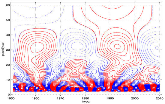
Figure 6. This contour, computed with frequency-domain method of CWT with data preparation method given in previously published papers, namely, $M=2^q,q={min}_{n\in Z}\{2^n>N\}$, manifests edge effect.

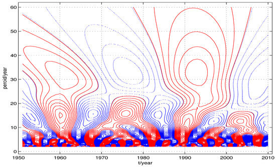
Figure 7. This contour, computed with the case 0 of Algorithm 3 with $M=N+2aT$, manifests no edge effect.

5. Conclusions

The continuous wavelet transform of a signal with finite length for a fixed scale is considered as a linear time-invariant operator. Furthermore, the filter with causal and stability is constructed. The algorithm of linear convolution constitutes a unifying framework to the continuous wavelet transform methods previously published in [17]. The precision of these methods based on this framework is almost the same, no matter what method is used, and higher than other methods that use the approximation of wavelet, for example, the $cwt$ function in wavelet toolbox of Matlab. The edge effect is also easily handled by using Equivalent Condition of Time-domain and Frequency-domain Algorithms of CWT.

The algorithms of CWT consist of two methods, time-domain method and frequency-domain method. For time-domain method, by constructing the causal filter ${\tilde{\psi }}_a\left(t\right)$, we know the wavelet coefficients are just the middle part of the corresponding linear convolution. For frequency-domain method, by exploring the relationship of ${\tilde{\psi }}_a\left(t\right)$ and ${\tilde{\tilde{\psi }}}_a\left(t\right)$, we know the wavelet coefficients are just the first N coefficients of the corresponding convolution. Furthermore, by constructing the different filters, the wavelet coefficients can be the first N coefficients, or the middle N coefficients, or the last N coefficients of the corresponding convolution for frequency-domain method.

There are three methods for the calculation of linear convolution. The first one is to directly implement the definition of linear convolution. The second one is known as the FFT-based method, for example, Algorithm 1. Lastly, if the length of the signal is far larger than the length of the filter, an overlap-add procedure for the calculation of linear convolution is faster than the previous two methods [23]. How to combine the Frequency-domain method and an overlap-add procedure for the computation of CWT is a question for future research.

References

- Huang, N.E.; Shen, Z.; Long, S.R.; Wu, M.C.; Shih, H.H.; Zheng, Q.; Yen, N.C.; Chi, C.T.; Liu, H.H. The empirical mode decomposition and the Hilbert spectrum for nonlinear and non-stationary time series analysis. Proc. Math. Phys. Eng. Sci. 1998, 454, 903–995. [Google Scholar] [CrossRef]
- Daubechies, I.; Heil, C. Ten Lectures on Wavelets. Comput. Phys. 1992, 6, 1671. [Google Scholar] [CrossRef]
- Gilles, J. Empirical Wavelet Transform. IEEE Trans. Signal Process. 2013, 61, 3999–4010. [Google Scholar] [CrossRef]
- Amezquita-Sanchez, J.P.; Adeli, H. A new music-empirical wavelet transform methodology for time frequency analysis of noisy nonlinear and non-stationary signals. Digit. Signal Process. 2015, 45, 55–68. [Google Scholar] [CrossRef]
- Daubechies, I.; Lu, J.; Wu, H.T. Synchrosqueezed wavelet transforms: An empirical mode decomposition-like tool. Appl. Comput. Harmon. Anal. 2011, 30, 243–261. [Google Scholar] [CrossRef]
- Garcia-Perez, A.; Amezquita-Sanche, J.P.; Dominguez-Gonzale, A.; Sedaghat, R.; Osornio-Rio, R.; Romero-Troncos, R.J. Fused empirical mode decomposition and wavelets for locating combined damage in a truss-type structure through vibration analysis. J. Zhejiang Univ. Sci. A 2013, 14, 615–630. [Google Scholar] [CrossRef]
- Boashash, B.; Khan, N.A.; Ben-Jabeur, T. Time frequency features for pattern recognition using high-resolution TFDs: A tutorial review. Digit. Signal Process. 2015, 40, 1–30. [Google Scholar]
- Glowacz, A. DC Motor Fault Analysis with the Use of Acoustic Signals, Coiflet Wavelet Transform, and K-Nearest Neighbor Classifier. Arch. Acoust. 2015, 40, 321–327. [Google Scholar] [CrossRef]
- Chen, J.; Rostami, J.; Tse, P.W.; Wan, X. The Design of a Novel Mother Wavelet that is Tailor-made for Continuous Wavelet Transform in Extracting Defect-Related Features from Reflected Guided Wave Signals. Measurement 2017, 110, 176–191. [Google Scholar] [CrossRef]
- Chamanzar, A.; Shabany, M.; Malekmohammadi, A.; Mohammadinejad, S. Efficient Hardware Implementation of Real-Time Low-Power Movement Intention Detector System Using FFT and Adaptive Wavelet Transform. IEEE Trans. Biomed. Circuits Syst. 2017, 11, 585–596. [Google Scholar] [CrossRef] [PubMed]
- Lee, W.K.; Ratnam, M.M.; Ahmad, Z.A. Detection of chipping in ceramic cutting inserts from workpiece profile during turning using fast Fourier transform (FFT) and continuous wavelet transform (CWT). Precis. Eng. 2017, 47, 406–423. [Google Scholar] [CrossRef]
- Ni, S.H.; Li, J.L.; Yang, Y.Z.; Yang, Z.T. An improved approach to evaluating pile length using complex continuous wavelet transform analysis. Insight Non-Destr. Test. Cond. Monit. 2017, 59, 318–324. [Google Scholar] [CrossRef]
- Rafiei, M.H.; Adeli, H. A novel unsupervised deep learning model for global and local health condition assessment of structures. Eng. Struct. 2018, 156, 598–607. [Google Scholar] [CrossRef]
- Perez-Ramirez, C.A.; Amezquita-Sanchez, J.P.; Adeli, H.; Valtierra-Rodriguez, M.; Camarena-Martinez, D.; Romero-Troncoso, R.J. New methodology for modal parameters identification of smart civil structures using ambient vibrations and synchrosqueezed wavelet transform. Eng. Appl. Artif. Intell. 2016, 48, 1–12. [Google Scholar] [CrossRef]
- Leigh, G.M. Fast FIR Algorithms for the Continuous Wavelet Transform From Constrained Least Squares. IEEE Trans. Signal Process. 2012, 61, 28–37. [Google Scholar] [CrossRef]
- Unser, M. Fast Gabor-like windowed Fourier and continuous wavelet transforms. IEEE Signal Process. Lett. 1994, 1, 76–79. [Google Scholar] [CrossRef]
- Yi, H.; Chen, Z.; Cao, Y. High Precision Computation of Morlet Wavelet Transform for Multi-period Analysis of Climate Data. J. Inf. Comput. Sci. 2014, 11, 6369–6385. [Google Scholar] [CrossRef]
- Torrence, C.; Compo, G.P. A Practical Guide to Wavelet Analysis. Bull. Am. Meteorol. Soc. 1998, 79, 61–78. [Google Scholar] [CrossRef]
- Burrus, C.; Parks, T.W. DFT/FFT and Convolution Algorithms: Theory and Implementation; John Wiley & Sons Inc.: New York, NY, USA, 1991. [Google Scholar]
- Jin, X.Q. Preconditioning Techniques for Toeplitz Systems; Higher Education Press: Beijing, China, 2010. [Google Scholar]
- Nagy, J.G.; Plemmons, R.J.; Torgersen, T.C. Iterative image restoration using approximate inverse preconditioning. IEEE Trans. Image Process. 1996, 5, 1151–1162. [Google Scholar] [CrossRef] [PubMed]
- Proakis, J.G.; Manolakis, D.G. Digital Signal Processing: Principles, Algorithms, And Applications; Pearson Education: Delhi, India, 2007; Volume 23, pp. 392–394. [Google Scholar]
- Mallat, S.G. A Wavelet Tour of Signal Processing: The Sparse Way; Academic Press: New York, NY, USA, 2009. [Google Scholar]
- Yi, H.; Shu, H. The improvement of the Morlet wavelet for multi-period analysis of climate data. Comptes Rendus Geosci. 2012, 344, 483–497. [Google Scholar] [CrossRef]
- Jones, D.L.; Baraniuk, R.G. Efficient approximation of continuous wavelet transforms. Electron. Lett. 1991, 27, 748–750. [Google Scholar] [CrossRef]
- Zhao, Y.Y.; Yuan, X.; Wei, Y.H. Realization of Continuous Wavelet Transform of Sequences by MATLAB. J. Sichuan Univ. 2006, 43, 325–329. [Google Scholar]
© 2018 by the authors. Licensee MDPI, Basel, Switzerland. This article is an open access article distributed under the terms and conditions of the Creative Commons Attribution (CC BY) license (http://creativecommons.org/licenses/by/4.0/).