Finite Difference Algorithm on Non-Uniform Meshes for Modeling 2D Magnetotelluric Responses

Abstract

A finite-difference approach with non-uniform meshes was presented for simulating magnetotelluric responses in 2D structures. We presented the calculation formula of this scheme from the boundary value problem of electric field and magnetic field, and compared finite-difference solutions with finite-element numerical results and analytical solutions of a 1D model. First, a homogeneous half-space model was tested and the finite-difference approach can provide very good accuracy for 2D magnetotelluric modeling. Then we compared them to the analytical solutions for the two-layered geo-electric model; the relative errors of the apparent resistivity and the impedance phase were both increased when the frequency was increased. To conclude, we compare our finite-difference simulation results with COMMEMI 2D-0 model with the finite-element solutions. Both results are in close agreement to each other. These comparisons can confirm the validity and reliability of our finite-difference algorithm. Moreover, a future project will extend the 2D structures to 3D, where non-uniform meshes should perform especially well.

1. Introduction

The magnetotelluric method is a passive electromagnetic exploration technique that measures orthogonal components of the electric and magnetic fields on the Earth’s surface [1]. The field source is naturally generated by variations in Earth’s magnetic field, which provide a wide and continuous spectrum of electromagnetic field waves. These fields induce currents into the Earth, which are measured at the surface and contain information about subsurface resistivity structures. With rapid advances in numerical modeling and ill-posed regularized inversion, the magnetotelluric method has become one of the most important tools for geophysical exploring [2,3].

The magnetotelluric numerical modeling aims to solve the boundary value problem derived from frequency-domain Maxwell’s equations and calculate the spatial distribution of electric and magnetic fields in the subsurface for a given conductivity distribution and a range of frequencies. Numerical modeling approaches such as finite difference (FD), finite element (FE), have been developed and applied as the process of forward modeling for 2D magnetotelluric regularized inversion [4,5,6,7,8]. The FD method based upon the differential form of the partial differential equations (PDEs) is to be solved. Each derivative can be replaced with an approximate difference formula and the computational domain is usually divided into rectangular cells. The efficiency and accuracy of the FD method for modeling magnetotelluric responses were proven for the 2D geo-electric model [9,10]. The FE method is another numerical approach that is often used for 2D and 3D magnetotelluric modeling, which involves assumed functional forms for the model and fields in small regions of specified geometry [11,12,13,14]. The FE method is more accurate for modeling a complicated medium, especially for topography, because of the greater flexibility of mesh discretization. Meanwhile, there are some different approaches to the numerical approximation of the 2D magnetotelluric forward problem [15,16,17,18]. There are some comprehensive reviews of these numerical methods and their advantages and disadvantages [19,20]. The references stated here represent a general view on magnetotelluric modeling.

In this paper, a non-uniform mesh approach in the FD numerical method was presented for a general 2D magnetotelluric modeling. The main challenge in applying the method for solving the magnetotelluric boundary value problem is to calculate spatial derivatives. To verify the accuracy of the FD forward algorithm, the resulting numerical was compared to both an analytical solutions and the FE numerical solutions.

2. Governing Equations

2.1. Electromagnetic Equations

Considering a right-handed coordinate system, with z-axis pointing downwards and x-axis along geo-electrical strike, and assuming time dependence as $e^{-\mathrm{i}\omega t}$ and neglecting displacement currents, electromagnetic Maxwell’s equations can be expressed in the frequency domain as [21]

$$\nabla \times E=\mathrm{i}\omega \mu H,$$

(1)

$$\nabla \times H=\sigma E.$$

(2)

where E is electric field and H is magnetic field. $\omega$ is an angular frequency ($\omega =2\pi /T$, T is a period). $\mu$ is the magnetic permeability in free space and $\mu ={\mu }_0=4\pi \times {10}^{-7} \mathrm{H}/\mathrm{m}$. $\sigma$ is the electric conductivity in ($\mathrm{S}/\mathrm{m}$) and is varied only in the direction of the y-axis and z-axis; i.e., $\sigma =\sigma \left(y,z\right)$.

For a 2D conductivity structure assuming the x-axis is the geo-electrical strike direction (i.e., $\partial E/\partial x\equiv 0$ and $\partial H/\partial x\equiv 0$), expanding the curl operators in Equations (1) and (2), the governing Maxwell’s equations are given by

$$\{\begin{array}{l}\frac{\partial E_z}{\partial y}-\frac{\partial E_y}{\partial z}=\mathrm{i}\omega \mu H_x,\\ E_y=\frac{1}{\sigma }\frac{\partial H_x}{\partial z},\\ E_z=-\frac{1}{\sigma }\frac{\partial H_x}{\partial y}.\end{array}\mathrm{TM}\text{-}\mathrm{mode}$$

(3)

and

$$\{\begin{array}{l}\frac{\partial H_z}{\partial y}-\frac{\partial H_y}{\partial z}=\sigma E_x,\\ H_y=\frac{1}{\mathrm{i}\omega \mu }\frac{\partial E_x}{\partial z},\\ H_z=-\frac{1}{\mathrm{i}\omega \mu }\frac{\partial E_x}{\partial y}.\end{array}\mathrm{TE}\text{-}\mathrm{mode}$$

(4)

These two modes are commonly referred to as transverse magnetic (TM) mode and transverse magnetic electric (TE) mode. We calculate the magnetic field $H_x$ (TM-mode) or electric field $E_x$ (TE-mode) parallel to the geo-electrical strike of the conductivity model. According to Equations (3) and (4), the associated partial differential equations can be written as

$$\frac{\partial }{\partial y}(\frac{1}{\sigma }\frac{\partial H_x}{\partial y})+\frac{\partial }{\partial z}(\frac{1}{\sigma }\frac{\partial H_x}{\partial z})+\mathrm{i}\omega \mu H_x=0,$$

(5)

$$\frac{\partial }{\partial y}(\frac{1}{\mathrm{i}\omega \mu }\frac{\partial E_x}{\partial y})+\frac{\partial }{\partial z}(\frac{1}{\mathrm{i}\omega \mu }\frac{\partial E_x}{\partial z})+\sigma E_x=0.$$

(6)

According to these relations, the magnetotelluric impedances for the TM and TE modes are

$$Z_{yx}=Z_{TM}=\frac{E_y}{H_x},Z_{xy}=Z_{TE}=\frac{E_x}{H_y}.$$

(7)

The associated apparent resistivities and impedance phases can be calculated as

$${\rho }_{a,ij}=\frac{1}{\omega \mu }{\left|Z_{ij}\right|}^2,ij=xy,ij=yx,$$

(8)

$${\varphi }_{ij}=\arctan \left[\frac{\mathrm{Im}\left(Z_{ij}\right)}{\mathrm{Re}\left(Z_{ij}\right)}\right].$$

(9)

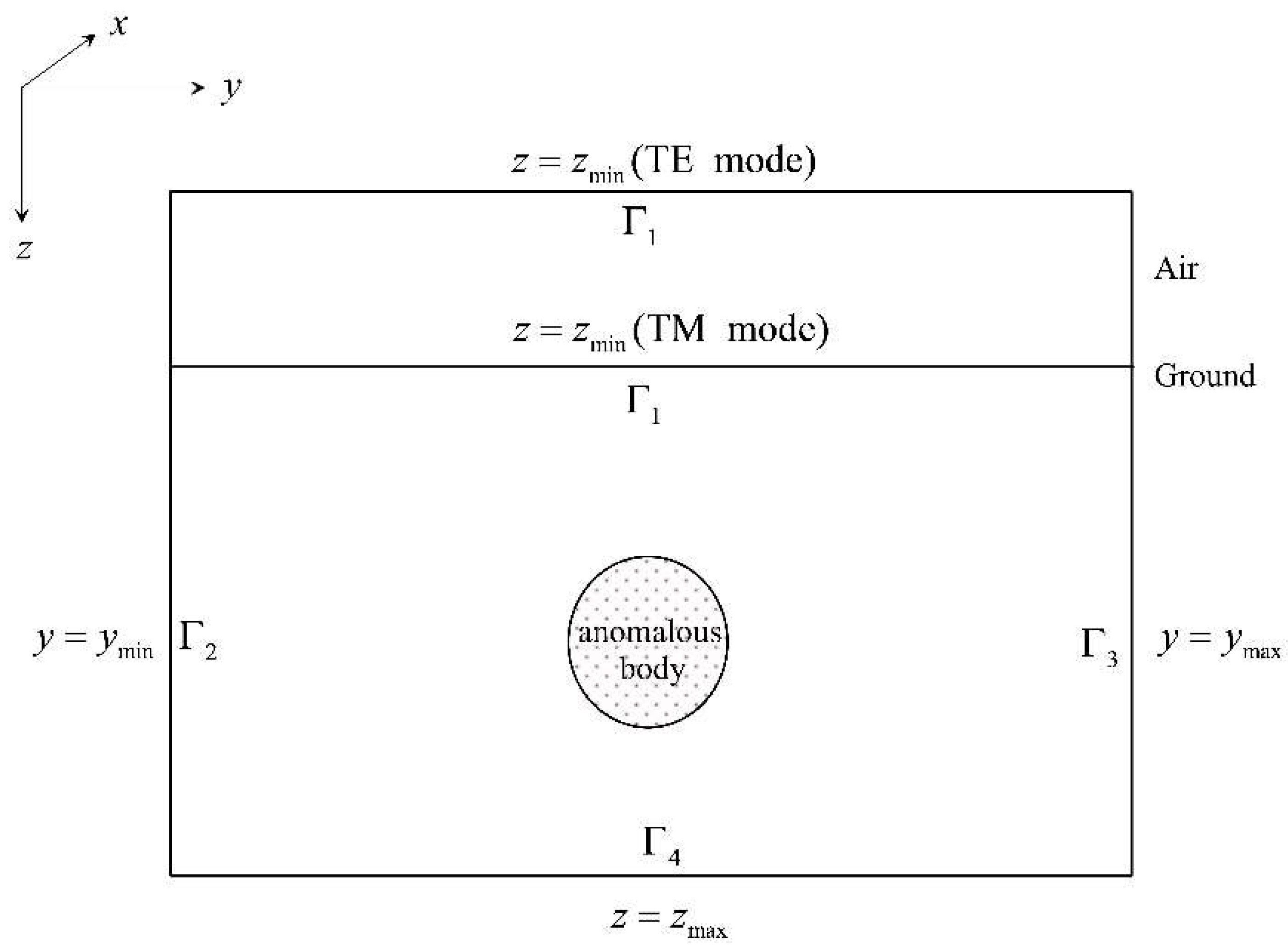
2.2. Boundary Conditions

For the TE-mode, the numerical domain is composed of both the air space and the subsurface earth. For the TM-mode, the magnetic field $H_x$ is nearly unchanged in the air space, so the air space can be eliminated from the computational domain [22]. To complete the boundary problem of the H-polarization, we must supply the boundary conditions for the magnetic field component on the outer boundaries. We restrict the computational domain for Equations (5) and (6) to 2D bounded domain $\mathsf{\Omega }=\left[y_{\min },y_{\max }\right]\times \left[z_{\min },z_{\max }\right]$, as shown in Figure 1. The computational domain is reduced to an isolated rectangular block with suitable boundary conditions, Then, we can divide the boundary of the computational domain $\mathsf{\Omega }$ can be divided into four parts expressed as follows: ${\mathsf{\Gamma }}_1=\left\{\left(y,z\right)|y_{\min }<y<y_{\max },z=z_{\min }\right\}$, ${\mathsf{\Gamma }}_2=\left\{\left(y,z\right)|z_{\min }<z<z_{\max },y=y_{\min }\right\}$, ${\mathsf{\Gamma }}_3=\left\{\left(y,z\right)|z_{\min }<z<z_{\max },y=y_{\max }\right\}$, and ${\mathsf{\Gamma }}_4=\left\{\left(y,z\right)|y_{\min }<y<y_{\max },z=z_{\max }\right\}$. We impose Dirichlet ${\mathsf{\Gamma }}_1$, Neumann ${\mathsf{\Gamma }}_2$, Neumann ${\mathsf{\Gamma }}_3$, and Robin ${\mathsf{\Gamma }}_4$ boundary conditions on the computational domain.

3. Forward Algorithm

3.1. FD Representation for 2D Magnetotelluric Problem

Before we can solve Equations (5) and (6), it is necessary to split the computational area into a mesh with $\left(N_{zb}+N_{za}\right)\times N_y$ cells, where $N_y$ is the number of cells in the horizontal direction and $N_{zb}$ and $N_{za}$ denote the number of cells in the vertical direction for the subsurface and the air, respectively. A resistivity value is assigned to each cell or each node.

The FD approximation is the simplest form of electromagnetic modeling. In order to construct FD scheme for solving Equations (5) and (6), non-uniform meshes shown in Figure 2 are constructed. In the TM-mode, approximation of second-order derivatives for Equation (5) can be expressed as

$$\begin{array}{ll}{\left[\frac{\partial }{\partial y}\left(\sigma \frac{\partial u}{\partial y}\right)\right]}_{i,j}& \approx \frac{1}{\frac{\Delta y_i+\Delta y_{i+1}}{2}}\left[{\left(\sigma \frac{\partial u}{\partial y}\right)}_{i+1,j}-{\left(\sigma \frac{\partial u}{\partial y}\right)}_{i,j}\right]\\ & \approx \frac{\frac{{\sigma }_{i,j}+{\sigma }_{i+1,j}}{2}\frac{u_{i+1,j}-u_{i,j}}{\frac{\Delta y_i+\Delta y_{i+1}}{2}}-\frac{{\sigma }_{i-1,j}+{\sigma }_{i,j}}{2}\frac{u_{i,j}-u_{i-1,j}}{\frac{\Delta y_{i-1}+\Delta y_i}{2}}}{\frac{\Delta y_i+\Delta y_{i+1}}{2}}\\ & =\frac{2\left({\sigma }_{i,j}+{\sigma }_{i+1,j}\right)\left(u_{i+1,j}-u_{i,j}\right)}{{\left(\Delta y_i+\Delta y_{i+1}\right)}^2}-\frac{2\left({\sigma }_{i-1,j}+{\sigma }_{i,j}\right)\left(u_{i,j}-u_{i-1,j}\right)}{\left(\Delta y_{i-1}+\Delta y_i\right)\left(\Delta y_i+\Delta y_{i+1}\right)}\end{array}$$

(10)

and

$${\left[\frac{\partial }{\partial y}\left(\sigma \frac{\partial u}{\partial y}\right)\right]}_{i,j}\approx \frac{2\left({\sigma }_{i,j}+{\sigma }_{i,j+1}\right)\left(u_{i,j+1}-u_{i,j}\right)}{{\left(\Delta z_j+\Delta z_{j+1}\right)}^2}-\frac{2\left({\sigma }_{i,j-1}+{\sigma }_{i,j}\right)\left(u_{i,j}-u_{i,j-1}\right)}{\left(\Delta z_{j-1}+\Delta z_j\right)\left(\Delta z_j+\Delta z_{j+1}\right)}$$

(11)

Substituting Equations (10) and (11) into Equation (5), the difference equation for TM-mode can be written as

$$\begin{array}{l}\frac{2\left({\sigma }_{i,j}+{\sigma }_{i+1,j}\right)\left(u_{i+1,j}-u_{i,j}\right)}{{\left(\Delta y_i+\Delta y_{i+1}\right)}^2}-\frac{2\left({\sigma }_{i-1,j}+{\sigma }_{i,j}\right)\left(u_{i,j}-u_{i-1,j}\right)}{\left(\Delta y_{i-1}+\Delta y_i\right)\left(\Delta y_i+\Delta y_{i+1}\right)}+\\ \frac{2\left({\sigma }_{i,j}+{\sigma }_{i,j+1}\right)\left(u_{i,j+1}-u_{i,j}\right)}{{\left(\Delta z_j+\Delta z_{j+1}\right)}^2}-\frac{2\left({\sigma }_{i,j-1}+{\sigma }_{i,j}\right)\left(u_{i,j}-u_{i,j-1}\right)}{\left(\Delta z_{j-1}+\Delta z_j\right)\left(\Delta z_j+\Delta z_{j+1}\right)}+\mathrm{i}\omega \mu u_{i,j}=0\end{array}$$

(12)

In the TE-mode, the difference equation resulting from approximation of Equation (6) is:

$$\begin{array}{ll}{\left[\frac{\partial }{\partial y}\left(\frac{\partial u}{\partial y}\right)\right]}_{i,j}& \approx \frac{1}{\frac{\Delta y_i+\Delta y_{i+1}}{2}}\left[{\left(\frac{\partial u}{\partial y}\right)}_{i+1,j}-{\left(\frac{\partial u}{\partial y}\right)}_{i,j}\right]\\ & \approx \frac{\frac{u_{i+1,j}-u_{i,j}}{\frac{\Delta y_i+\Delta y_{i+1}}{2}}-\frac{u_{i,j}-u_{i-1,j}}{\frac{\Delta y_{i-1}+\Delta y_i}{2}}}{\frac{\Delta y_i+\Delta y_{i+1}}{2}}\end{array}$$

(13)

and

$${\left[\frac{\partial }{\partial z}\left(\frac{\partial u}{\partial z}\right)\right]}_{i,j}\approx \frac{\frac{u_{i,j+1}-u_{i,j}}{\frac{\Delta z_j+\Delta z_{j+1}}{2}}-\frac{u_{i,j}-u_{i,j-1}}{\frac{\Delta z_{j-1}+\Delta z_j}{2}}}{\frac{\Delta z_j+\Delta z_{z+1}}{2}}$$

(14)

Therefore, substituting Equations (13) and (14) into Equation (6), the difference equation for TE-mode can be written as

$$\frac{\frac{u_{i+1,j}-u_{i,j}}{\frac{\Delta y_i+\Delta y_{i+1}}{2}}-\frac{u_{i,j}-u_{i-1,j}}{\frac{\Delta y_{i-1}+\Delta y_i}{2}}}{\frac{\Delta y_i+\Delta y_{i+1}}{2}}+\frac{\frac{u_{i,j+1}-u_{i,j}}{\frac{\Delta z_j+\Delta z_{j+1}}{2}}-\frac{u_{i,j}-u_{i,j-1}}{\frac{\Delta z_{j-1}+\Delta z_j}{2}}}{\frac{\Delta z_j+\Delta z_{z+1}}{2}}+\mathrm{i}\omega \mu {\sigma }_{i,j}{u}_{i,j}=0$$

(15)

The solution vector u, which represents the components $H_x$ or $E_x$ for the different mesh nodes, is rewritten by

$$u=\left(\begin{array}{c}{u}_1=u_{1,1}\\ u_2=u_{1,2}\\ ⋮\\ u_{\left(i-1\right)\times \left(Ny+1\right)+j}=u_{i,j}\\ ⋮\\ u_{Nz\times \left(Ny+1\right)+Ny}=u_{Nz+1,Ny}\\ u_{\left(Nz+1\right)\times \left(Ny+1\right)}=u_{Nz+1,Ny+1}\end{array}\right),$$

(16)

Considering boundary conditions of the 2D magnetotelluric forward problem, the resulting linear system of equations in the form

$$Ku=s.$$

(17)

gives a numerical solution of Equations (5) and (6). Where K is the system matrix containing electrical parameters $\sigma$, and the right-side column vector s contains information related to boundary conditions. Equation (17) can be solved by the direct solver for a sparse matrix in MATLAB. Finally, the magnetotelluric responses including impedance, apparent resistivity and phase at each site for each frequency are calculated by Equations (7)–(9).

The subroutines described here for calculating magnetotelluric responses, given in Appendix A and Appendix B, were developed in MATLAB.

3.2. Benchmark with Homogeneous Half-Space

To test the accuracy of our FD algorithm, a homogeneous half-space model is illustrated for TM-mode. The size of computational domain was designed as 20 km × 5 km. The model was homogeneous with a conductivity of 0.1 S/m. We supposed that there is one magnetotelluric site located on the surface (z = 0 km). The magnetotelluric responses of the magnetic field H_x are computed in the frequency range 0.001 to 1000 Hz. The given domain was discretized into many meshes and nodes with non-uniform approach. According to the information of mesh generation, the number of nodes in y-axis and z-axis are set as 51 and 41, respectively. The total numbers of nodes generated were 2091.

The numerical results of the homogeneous half-space are shown in Figure 3. It is obvious that the magnetic field H_x including its real part and imaginary part computed by the FD method with non-uniform meshes are good agree with the analytical solution. The numerical results indicate that our FD approach can provide very good accuracy for 2D magnetotelluric modeling.

4. Numerical Results

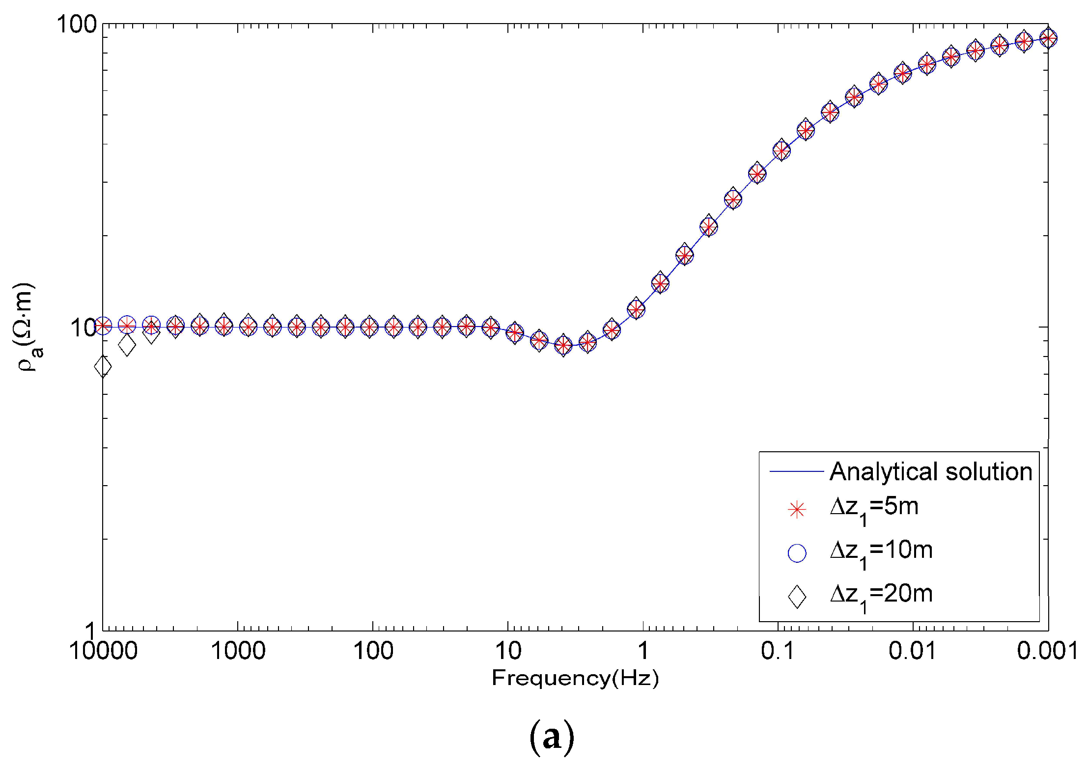
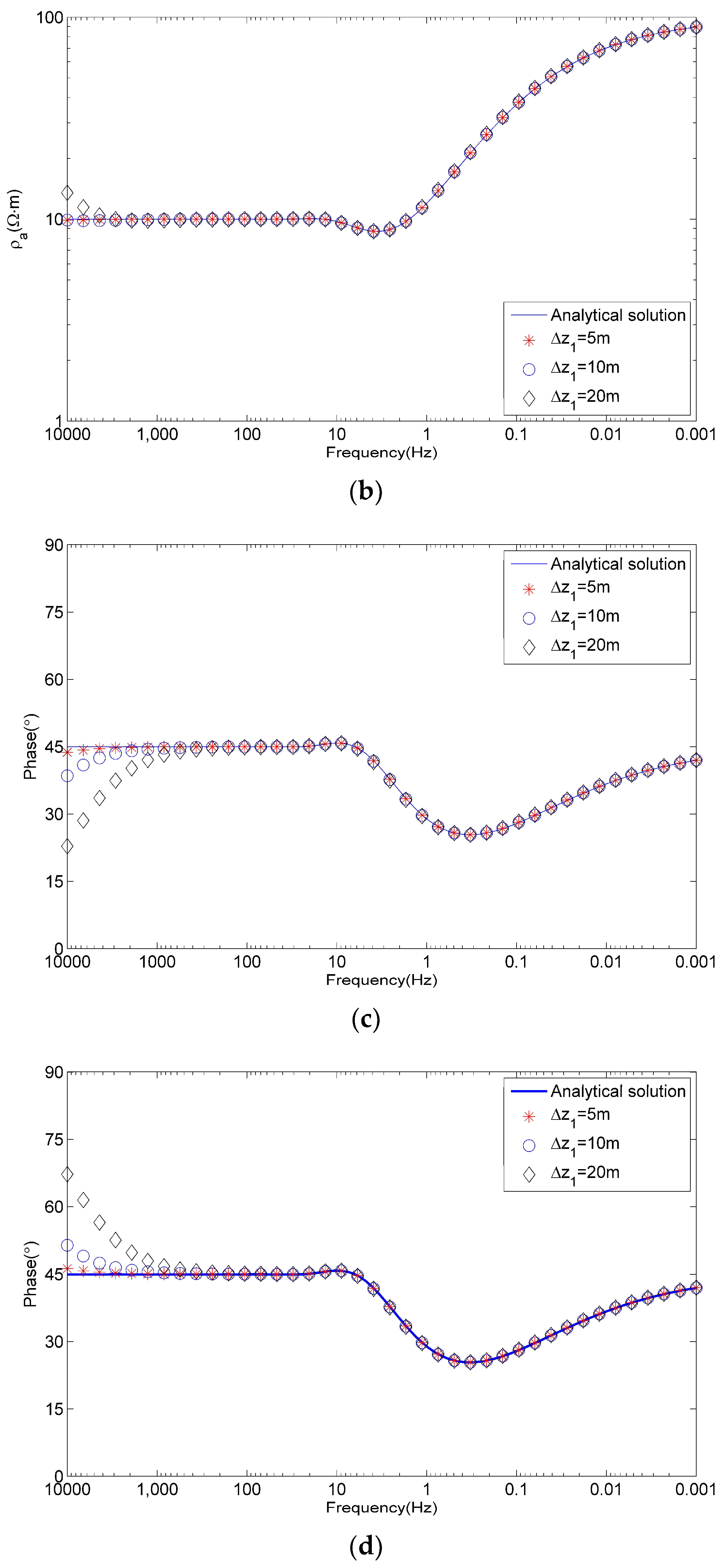
4.1. Comparison of FD Results and Analytical Solutions

The two-layered model is used as a test example for the comparison of FD numerical solution and analytical solution. It is supposed that the 1D geo-electric model includes two resistivity layers. The thickness of the top layer is 1 km, and its resistivity value is assumed to be 10 ohm-m. For the bottom layer, its thickness and resistivity value are assumed to be 1 km and 100 ohm-m. The computational size of the model is set as 20 km × 2 km.

The results of the two-layered model are shown in Figure 4. It is obvious that relative errors of the apparent resistivities and the impedance phases were both increased when the frequency was increased, with the maximum error at the longest frequency 1000 Hz and the minimum at the shortest frequency 0.001 Hz. At the highest frequency, the vertical grid spacing size at earth’s surface must be small enough so that the linear approximation of the electric field is reasonably close to the exponential decay of the electromagnetic fields. Through the numerical examples, the first vertical mesh size should be suggested approximately 1/3 of the shortest skin depth of the top layer.

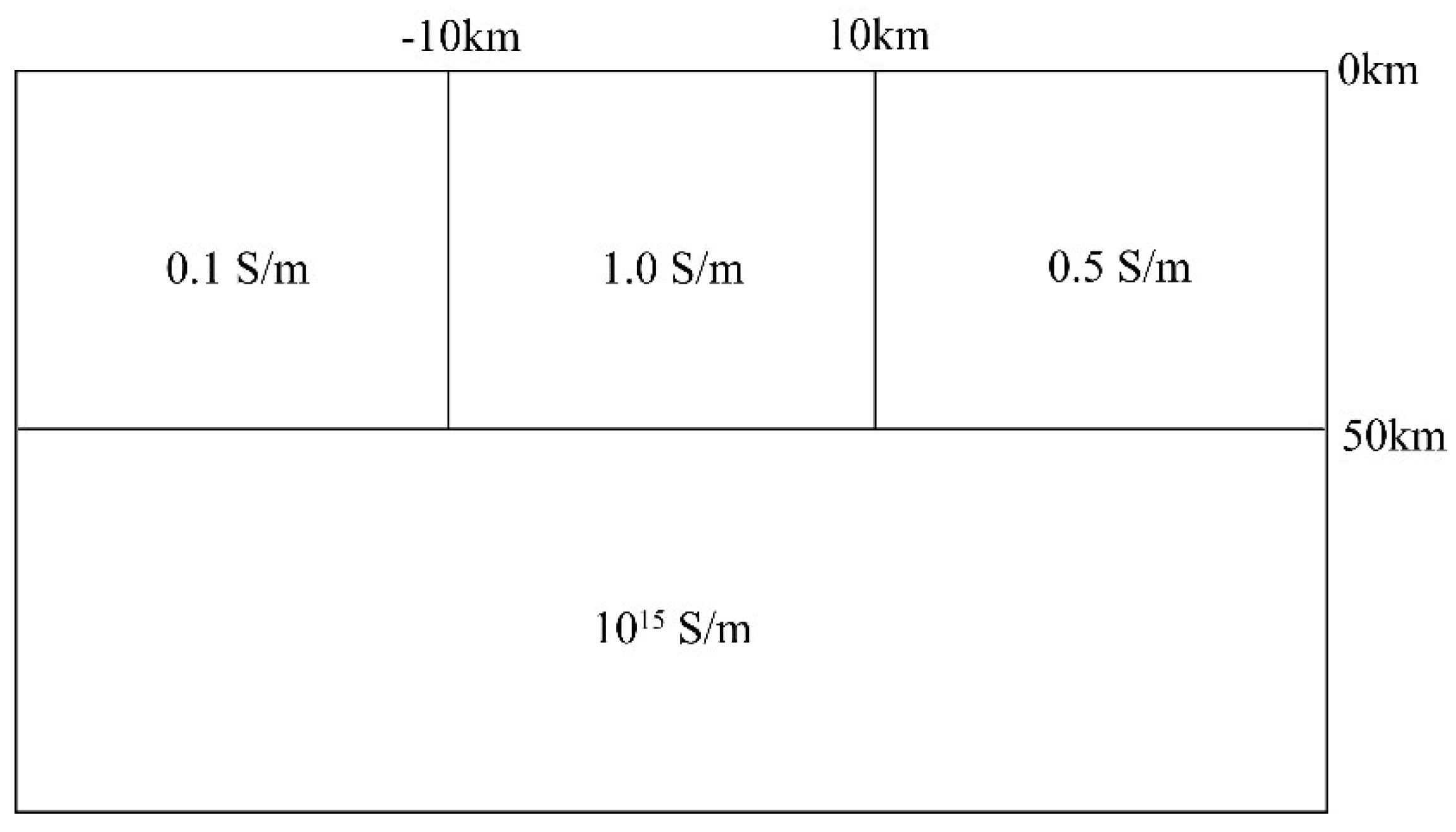
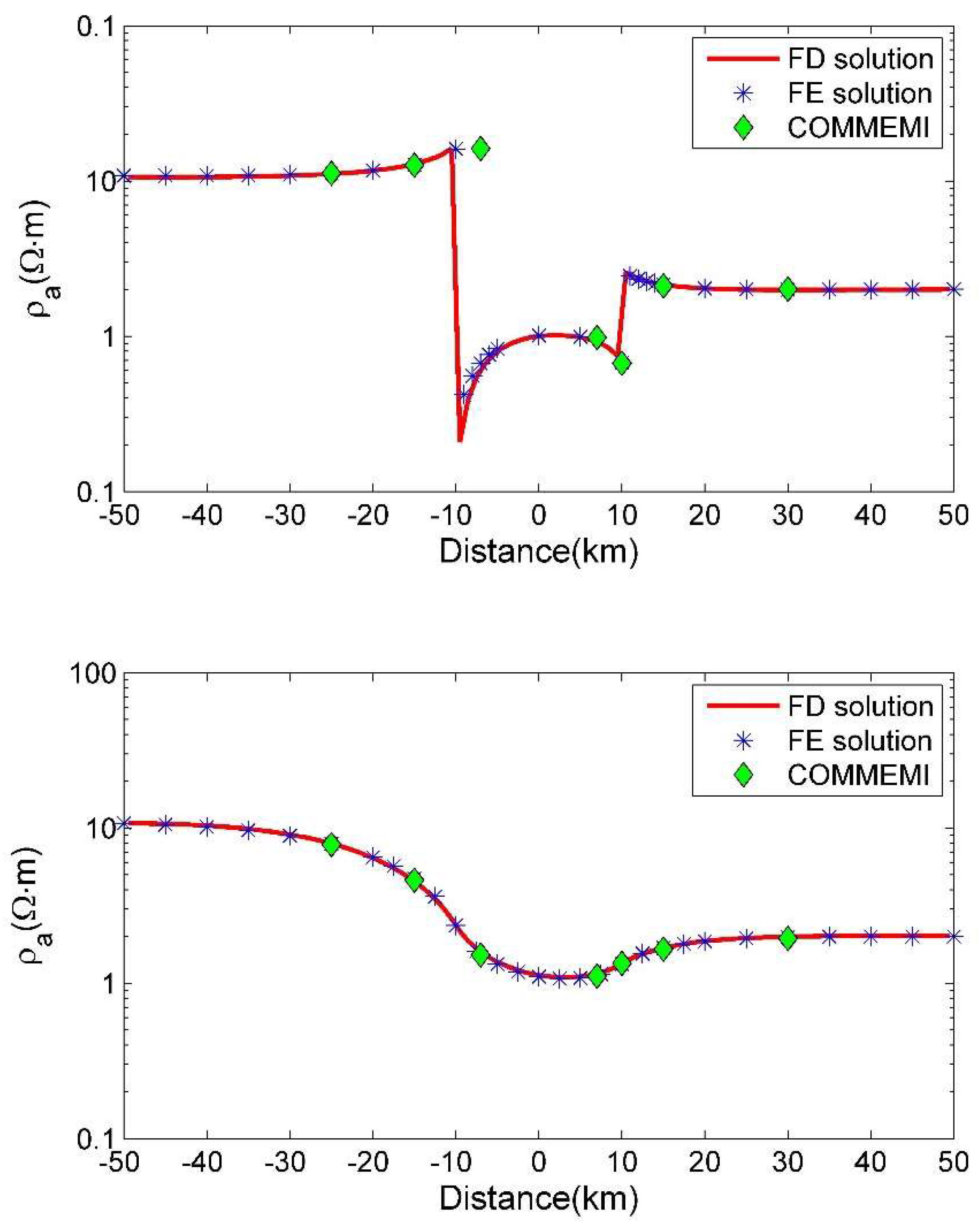
4.2. Comparison of FD Results and FE Solutions

In this section, the reliability of the non-uniform meshes FD algorithm is confirmed by the COMMEMI 2D-0 testing model. The COMMEMI 2D-0 model, proposed by Zhdanov et al. for comparing of numerical modeling methods for electromagnetic induction [19], is illustrated in Figure 5. It consists of three segments of different conductivities with horizontal contrasts of 1:10 and 2:1, lying on a perfectly conducting basement.

With a testing period of 30 s, the simulated apparent resistivities by the presented FD approach are compared with the FE solution [7] and the averaged volume integral results from the COMMEMI project [19]. The computational size of magnetotelluric domain was designed as 100 km × 100 km. Using the technique of the non-uniform meshes, we set discrete elements in given domain as 100 × 80 (i.e., N_y = 100 and N_z = 80), and extended 50 km to air space for TE-mode. Figure 6 shows the results of the FD computations along a profile.

One can see (Figure 6) that the results calculated by the FD method and the FE method are in close agreement to each other. It shows that the apparent resistivities have no significant difference. Compared to the FE solution, the average relative error for the apparent resistivity is 0.05, which are in the acceptance limits. Meanwhile, our FD numerical results were quite comparable those of the COMMEMI 2D-0 projects.

5. Conclusions

The finite difference method with non-uniform meshes has been adapted to simulate the 2D magnetotelluric responses. We presented the calculation formula of this approach from the boundary value problem of electromagnetic fields. In the first investigation, the benchmark of a finite-difference algorithm was tested by a homogeneous half-space model and the approach of non-uniform meshes can provide very good accuracy for 2D magnetotelluric modeling. Compared to the analytical solutions for a 1D geo-electric model, the relative errors of the apparent resistivity and the impedance phase were both increased when the frequency was increased. Meanwhile, the relative errors were reduced when the mesh size was reduced. The reason can be attributed to the accuracy of the FD calculation for the apparent resistivity and the impedance phase depends on the vertical grid spacing size of the near-surface. Furthermore, we presented the COMMEMI 2D-0 model in comparison to results derived by the FE calculation. Both results are in close agreement to each other. These comparisons demonstrate that our FD algorithm can be valid and reliable.

References

- Cagniard, L. Basic theory of the magneto-telluric method of geophysical prospecting. Geophysics 1953, 18, 605–645. [Google Scholar] [CrossRef]
- Lee, T.J.; Han, N.; Song, Y. Magnetotelluric survey applied to geothermal exploration: An example at Seokmo Island, Korea. Explor. Geophys. 2010, 41, 61–68. [Google Scholar] [CrossRef]
- Barcelona, H.; Favetto, A.; Peri, V.G.; Pomposiello, C.; Ungarelli, C. The potential of audiomagnetotellurics in the study of geothermal fields: A case study form the northern segment of the La Candelaria Range, northwestern Argentina. J. Appl. Geophys. 2013, 88, 83–93. [Google Scholar] [CrossRef]
- DeGroot-HedlinN, C.; Constable, S. Occam’s inversion to generate smooth, two-dimensional models from magnetotelluric data. Geophysics 1990, 55, 1613–1624. [Google Scholar] [CrossRef]
- Rodi, W.; Mackie, R.L. Nonlinear conjugate gradient algorithm for 2-D magnetotelluric inversion. Geophysics 2001, 66, 174–187. [Google Scholar] [CrossRef]
- Siripunvaraporn, W.; Egbert, G.D. Data space conjugate gradient inversion for 2-D magnetotelluric data. Geophys. J. Int. 2007, 170, 986–994. [Google Scholar] [CrossRef]
- Lee, S.K.; Kim, H.J.; Song, Y.; Lee, C.K. MT2Dinvmatlab—A program in MATLAB and FORTRAN for two-dimensional magnetotelluric inversion. Comput. Geosci. 2009, 35, 1722–1734. [Google Scholar] [CrossRef]
- Kelbert, A.; Meqbel, N.; Egbert, G.D.; Tandon, K. ModEM: A modular system for inversion of electromagnetic geophysical data. Comput. Geosci. 2014, 66, 40–53. [Google Scholar] [CrossRef]
- Pek, J.; Verner, T. Finite-difference modelling of magnetotelluric fields in two-dimensional anisotropic media. Geophys. J. Int. 1997, 128, 505–521. [Google Scholar] [CrossRef]
- Kalscheuer, T.; Juhojuntti, N.; Vaittinen, K. Two-dimensional magnetotelluric modelling of Ore deposits: Improvements in model constraints by inclusion of borehole measurements. Surv. Geophys. 2018, 39, 467–507. [Google Scholar] [CrossRef]
- Wannamaker, P.E.; Stodt, J.A.; Rijo, L. Two-dimensional topographic responses in magnetotellurics modeled using finite elements. Geophysics 1986, 51, 2131–2144. [Google Scholar] [CrossRef]
- Franke, A.; Börner, R.U.; Spitzer, K. Adaptive unstructured grid finite element simulation of two-dimensional magnetotelluric fields for arbitrary surface and seafloor topography. Geophys. J. Int. 2007, 171, 71–86. [Google Scholar] [CrossRef]
- Key, K.; Weiss, C. Adaptive finite-element modeling using unstructured grids: The 2D magnetotelluric example. Geophysics 2007, 71, 291–299. [Google Scholar] [CrossRef]
- Sarakorn, W. 2-D magnetotelluric modeling using finite element method incorporating unstructured quadrilateral elements. J. Appl. Geophys. 2017, 139, 16–24. [Google Scholar] [CrossRef]
- Wittke, J.; Tezkan, B. Meshfree magnetotelluric modelling. Geophys. J. Int. 2014, 198, 1255–1268. [Google Scholar] [CrossRef]
- Du, H.K.; Ren, Z.Y.; Tang, J.T. A finite-volume approach for 2D magnetotellurics modeling with arbitrary topographies. Stud. Geophys. Geod. 2016, 60, 332–347. [Google Scholar] [CrossRef]
- Bihlo, A.; Farquharson, C.G.; Haynes, R.D.; Loredo-Osti, J.C. Probabilistic domain decomposition for the solution of the two-dimensional magnetotelluric problem. Comput. Geosci. 2017, 21, 117–129. [Google Scholar] [CrossRef]
- Sarakorn, W.; Vachiratienchai, C. Hybrid finite difference-finite element method to incorporate topography and bathymetry for two-dimensional magnetotelluric modeling. Earth Planets Space 2018, 70, 70–103. [Google Scholar] [CrossRef]
- Zhdanov, M.S.; Varentsov, I.M.; Weaver, J.T.; Golubev, N.G.; Krylov, V.A. Methods for modelling electromagnetic fields results from COMMEMI—The international project on the comparison of modelling methods for electromagnetic induction. J. Appl. Geophys. 1997, 37, 133–271. [Google Scholar] [CrossRef]
- Varilsüha, D.; Candansayar, M.E. 3D magnetotelluric modeling by using finite-difference method: Comparison study of different forward modeling approaches. Geophysics 2018, 83, 51–60. [Google Scholar] [CrossRef]
- Guo, Z.Q.; Egbert, G.D.; Wei, W.B. Modular implementation of magnetotelluric 2D forward modeling with general anisotropy. Comput. Geosci. 2018, 118, 27–38. [Google Scholar] [CrossRef]
- Aprea, C.; Booker, J.; Smith, J. The forward problem of electromagnetic induction: Accurate finite-difference approximations for two-dimensional discrete boundaries with arbitrary geometry. Geophys. J. Int. 1997, 129, 29–40. [Google Scholar] [CrossRef]
© 2018 by the authors. Licensee MDPI, Basel, Switzerland. This article is an open access article distributed under the terms and conditions of the Creative Commons Attribution (CC BY) license (http://creativecommons.org/licenses/by/4.0/).
Share and Cite
Tong, X.; Guo, Y.; Xie, W. Finite Difference Algorithm on Non-Uniform Meshes for Modeling 2D Magnetotelluric Responses. Algorithms 2018, 11, 203. https://doi.org/10.3390/a11120203
Tong X, Guo Y, Xie W. Finite Difference Algorithm on Non-Uniform Meshes for Modeling 2D Magnetotelluric Responses. Algorithms. 2018; 11(12):203. https://doi.org/10.3390/a11120203
Chicago/Turabian StyleTong, Xiaozhong, Yujun Guo, and Wei Xie. 2018. "Finite Difference Algorithm on Non-Uniform Meshes for Modeling 2D Magnetotelluric Responses" Algorithms 11, no. 12: 203. https://doi.org/10.3390/a11120203
APA StyleTong, X., Guo, Y., & Xie, W. (2018). Finite Difference Algorithm on Non-Uniform Meshes for Modeling 2D Magnetotelluric Responses. Algorithms, 11(12), 203. https://doi.org/10.3390/a11120203