Understanding and Enhancement of Internal Clustering Validation Indexes for Categorical Data

Abstract

Clustering is one of the main tasks of machine learning. Internal clustering validation indexes (CVIs) are used to measure the quality of several clustered partitions to determine the local optimal clustering results in an unsupervised manner, and can act as the objective function of clustering algorithms. In this paper, we first studied several well-known internal CVIs for categorical data clustering, and proved the ineffectiveness of evaluating the partitions of different numbers of clusters without any inter-cluster separation measures or assumptions; the accurateness of separation, along with its coordination with the intra-cluster compactness measures, can notably affect performance. Then, aiming to enhance the internal clustering validation measurement, we proposed a new internal CVI—clustering utility based on the averaged information gain of isolating each cluster (CUBAGE)—which measures both the compactness and the separation of the partition. The experimental results supported our findings with regard to the existing internal CVIs, and showed that the proposed CUBAGE outperforms other internal CVIs with or without a pre-known number of clusters.

1. Introduction

Clustering analysis is the unsupervised process of partitioning a group of data objects into clusters, with the objective to grouping objects of high similarity into the same cluster, while separating dissimilar objects into different clusters. Clustering is a main task of data analysis, and it has been studied extensively in the fields of data mining and machine learning [1,2]. Clustering techniques can be roughly distinguished as hard and soft clustering, this study is limited to the hard clustering analysis, in which each object belongs to one and only one cluster.

The results of clustering—partitions—vary with parameter settings, clustering methods, and the criteria of similarity (or dissimilarity) [3]. The mechanisms of the clustering method, such as random initialization, can cause inconsistencies in clustering results as well. How do we determine the final result from multiple possible partitions? As shown in Figure 1, the standard solution is to conduct several clustering processes with different schemes respectively, then select the partition of the highest quality [1,4,5]. The key is to define and measure the ‘quality of partitions’ by clustering validation indexes (CVIs) in the third step in Figure 1.

By whether to use external information, we can summarize the CVIs into two categories, i.e., external and internal CVIs. External CVIs use external information to evaluate the quality of the clustering results. For instance, if the prior knowledge, such as the true partition (or the partition designated by experts) exists, external CVIs can be used to evaluate the conformity of the clustered partition and the prior partition [6,7,8]. Such prior knowledge is absent in the unsupervised scenario, which makes the external CVIs inapplicable.

On the other hand, Internal CVIs require no such prior knowledge, and have extensive practical applications in information retrieval, text and image analysis, biological engineering, and other domains of data mining [9,10,11,12,13,14,15,16]. The quality of clustering results is usually inspected internally from two aspects—the intra-cluster compactness, and the inter-cluster separation (also known as isolation) [5,17,18,19,20,21,22,23]. The compactness reflects the degree of similarity of the objects in the same cluster, while the separation reflects how the objects in one cluster are dissimilar to others.

Meanwhile, the internal CVIs for numerical data, such as the Dunn index [24], the I index [25], the Silhouette index [26], and the Calinski-Harabasz index [27], use intuitive geometric information to evaluate the partitions, which makes them unsuitable for categorical data clustering. Considering the increasing amount of categorical data in practical applications and the challenging issues that have not been adequately addressed in the literature, further research on internal CVIs for categorical data is in need [9,14,15,28,29].

Therefore, in this paper, we limit our scope to provide insight and enhancement of the internal CVIs for categorical data:

• Do internal CVIs for categorical data show monotonicity with respect to the number of clusters? One should avoid the monotonicity in validation measurement to prevent the bias towards partitions with more clusters, which would leave the performance of the evaluation to the boundary of the number of clusters in the candidate partitions.
• Do internal CVIs for categorical data which use no separation measures really ignore the separation? A partition of good compactness is not necessarily a good partition, since the objects in one cluster may be similar to the objects in other clusters as well. Some internal CVIs for categorical data use no separation measures based on the attribute distribution between clusters, and have been proven to be effective when the number of clusters is constant in reference [9]. However, if the impact of separation on the clustering validation is ignored, the compactness measure alone may not be effective in evaluating partitions of different sizes due to the first issue.
• What can we offer to enhance performance? After research on the above issues, we wish to offer an alternative internal CVI that has improved performance on categorical data clustering validation measurement.

To better understand the internal CVIs for categorical data, we investigate five well-known internal CVIs for categorical data clustering validation evaluation, i.e., the information entropy function (E) [30], the k-modes objective function (F) [31], the category utility function (CU) [32], the objective function of clustering with slope (Clope_r) [33], and the objective function of categorical data clustering with subjective factors (R) [34]. We attempt to reveal the nature of the five internal CVIs by investigating the compactness measures and the separation measures, and discuss whether assumptions of separation exist and can be substituted for the separation measures. Meanwhile, we theoretically analyze whether the compactness measures for categorical data show monotonicity in certain circumstances, and the role of separation measures (assumptions) in neutralizing the monotonicity.

Then, to enhance the internal measurement, we propose a new internal CVI that has improved performance, namely, the clustering utility based on the averaged information gain of isolating each cluster (CUBAGE). CUBAGE uses the proposed averaged information gain of isolating each cluster (AGE) to measure the separation, and the reciprocal entropy of the dataset conditioned on the partition to measure the compactness.

The paper is organized into six sections. Section 2 is the related work. Section 3 provides in-depth analysis and discussions of five CVIs on the first two issues. In Section 4, we present the proposed internal CVI. Section 5 presents our experimental results and detailed discussion. Finally, we state our conclusions in Section 6.

2. Related Work

In this section, we first clarify our notations throughout this paper, then introduce some widely-used internal CVIs for categorical data. Additionally, we provide a brief comparison of internal and external CVIs.

2.1. Notations

Unless stated otherwise, we used the following notations in this paper. U = {X₁, …, X_n} is a set of n objects, each object is described by the same m independent attributes A₁, …, A_m. The value of attribute A_j (j = 1, …, m) can be taken only from domain D(A_j) = {a_j⁽¹⁾, …, a_j^(dj)}, where d_j is the number of possible values of the attribute. p(a_j⁽ⁱ⁾) is the probability of attribute A_j taking the value a_j⁽ⁱ⁾ (i = 1, …, d_j).

C ≠ Φ is a set of objects (or, a cluster), a partition P = {C₁, …, C_k} is the clustering result of U into k clusters, with the property that C₁ ∪ C₂ ∪ … ∪ C_k = U, and C_l ∩ C_l’ = Φ (l ≠ l’; l, l’ = 1, …, k). For any given C_l, the conditional probability of attribute A_j taking value a_j⁽ⁱ⁾ in cluster C_l is p(a_j⁽ⁱ⁾|C_l). D(A_j|C_l) is the domain of attribute A_j in cluster C_l, obviously, D(A_j|C_l) ⊆ D(A_j).

2.2. Internal Clustering Validation Indexes

1. The information entropy function (E).

The information entropy of a random variable indicates the information and uncertainty that the variable has [35]. Considering attribute A as a random categorical variable, the entropy H(A) is defined as follows:

$$H(A)=-{\displaystyle \sum _i^{d}p(a^{(i)})\log (p(a^{(i)}))}.$$

(1)

Given a set of independent variables V = {A₁, …, A_m}, the entropy H(V) is:

$$H(V)={\displaystyle \sum _j^{m}H(A_j)}=-{\displaystyle \sum _j^m{\displaystyle \sum _i^{d_j}p(a_j{}^{(i)})\log (p(a_j{}^{(i)}))}}.$$

(2)

A lower H(V) indicates less uncertainty of V.

Given a partition P = {C₁, …, C_k}, the entropy of V conditioned on P, i.e., H(V|P), is considered as the ‘whole entropy of the partition’ [30]:

$$\begin{array}{cc}\hfill E(P)=H(V|P)& =-{\displaystyle \sum _{j=1}^m{\displaystyle \sum _{l=1}^{k}p(C_l){\displaystyle \sum _{i=1}^{d_j}p(a_j{}^{(i)}|C_l)\log (p(a_j{}^{(i)}|C_l))}}}\hfill \\ & =-{\displaystyle \sum _{j=1}^m{\displaystyle \sum _{l=1}^k{\displaystyle \sum _{i=1}^{d_j}p(a_j{}^{(i)},C_l)\log (p(a_j{}^{(i)}|C_l))}}},\hfill \end{array}$$

(3)

where p(a_j⁽ⁱ⁾|C_l) is the conditional probability of the value a_j⁽ⁱ⁾, given cluster C_l. Notice that the probability of C_l is p(C_l) = |C_l|/n.

E(P) attempts to represent the total entropy of the partition, which can be construed as the degree of disorder, by summing the weighted entropy of each cluster. To minimize the function E(P) is to find a partition in which the values of attributes describing the objects in the same clusters are centralized, which indicates that the objects are more similar in each cluster.

2. The k-modes objective function (F).

Similar to the k-means clustering algorithm [36], k-modes compares each object in the same cluster with the cluster center, and sums the dissimilarities [31]. Since it is improper to take the means of categorical values as the cluster center, k-modes use the modes of values of each attribute. The dissimilarity between the object and the center is defined as:

$$d(X_{li},Z_l)={\displaystyle \sum _{j=1}^m\delta (x_{lij},z_{lj})},$$

(4)

where X_li is the ith object in cluster C_l, x_lij is the value of attribute A_j describing object X_i, Z_l is the center of cluster C_l, z_lj is the value of attribute A_j describing center Z_l, and:

$$\delta (x_{lij},z_{lj})=\{\begin{array}{c}\begin{array}{cc}1,& x_{lij}=z_{lj},\end{array}\\ \begin{array}{cc}0,& x_{lij}\ne z_{lj}.\end{array}\end{array}$$

(5)

Therefore, the k-modes objective function is:

$$F(P)={\displaystyle \sum _{l=1}^k{d}_{cluster}(C_l)}={\displaystyle \sum _{l=1}^k{\displaystyle \sum _{i=1}^{\left|C_l\right|}d(X_{li},Z_l)}}.$$

(6)

where d_cluster(C_l) is the sum of the dissimilarity between each object in cluster C_l and its center:

$$d_{cluster}(C_l)={\displaystyle \sum _{i=1}^{\left|C_l\right|}d(X_{li},Z_l)}=\left|C_l\right|\cdot {\displaystyle \sum _{j=1}^m[(1-{\max }_{i=1}^{d_j}p(a_j{}^{(i)}|C_l)]}.$$

(7)

F(P) describes the overall dissimilarities between objects and centers; a lower F(P) indicates that partition P has a higher quality.

3. The category utility function (CU).

For the objects in the same cluster, CU measures the possibility of these objects taking the same attribute values [32]:

$$\begin{array}{cc}\hfill CU(P)& ={\displaystyle \sum _{l=1}^{k}p(C_l){\displaystyle \sum _{j=1}^m{\displaystyle \sum _{i=1}^{d_j}[p{(a_j{}^{(i)}|C_l)}^2-p{(a_j{}^{(i)})}^2}}}]\hfill \\ & ={\displaystyle \sum _{l=1}^{k}p(C_l){\displaystyle \sum _{j=1}^m{\displaystyle \sum _{i=1}^{d_j}[p{(a_j{}^{(i)}|C_l)}^2}}}]-{\displaystyle \sum _{l=1}^k{\displaystyle \sum _{j=1}^m{\displaystyle \sum _{i=1}^{d_j}p{(a_j{}^{(i)})}^2}}}.\hfill \end{array}$$

(8)

This process attempts to maximize both the probability that two objects in the same category have attribute values in common by p(a_j⁽ⁱ⁾|C_l)², and the probability that objects from different categories have different attribute values by −p(a_j⁽ⁱ⁾)². However, the last term −p(a_j⁽ⁱ⁾)² is invariable when the dataset is given. Therefore:

$$CU(P)={\displaystyle \sum _{l=1}^{k}p(C_l){\displaystyle \sum _{j=1}^m{\displaystyle \sum _{i=1}^{d_j}[p{(a_j{}^{(i)}|C_l)}^2}}}]-Constant,$$

(9)

where C is a constant. This means that the CU only measures how similar the objects in the same cluster are.

The authors of references [37,38] further averaged the values of the CU(P) measure over clusters, i.e., they used CU(P)/k instead of CU(P) to compare the partitions of different size. In this paper, we refer to the modified function as CU_1/k(P).

4. The CLOPE objective function (Clope_r)

CLOPE is an efficient clustering algorithm for large scaled datasets, and the basic idea of its criterion function is simple and straightforward [33,39]. CLOPE first defined the size and the width of cluster C_l:

$$Size(C_l)={\displaystyle \sum _{j=1}^m{\displaystyle \sum _{i=1}^{d_j}Occ(a_j{}^{(i)},C_l)}},$$

(10)

$$Width(C_l)={\displaystyle \sum _{j=1}^m\left|D(A_j|C_l)\right|},$$

(11)

where Occ(a_j⁽ⁱ⁾|C_l) is the number of occurrences of value a_j⁽ⁱ⁾ in cluster C_l:

$$Occ(a_j{}^{(i)},C_l)=\left|C_l\right|\times p(a_j{}^{(i)}|C_l).$$

(12)

Then, the objective is to maximize the following function:

$$Clope(P)={\displaystyle \sum _{l=1}^{k}p(C_l)\frac{Size(C_l)}{Width{(C_l)}^r}},$$

(13)

where r is the parametric power.

Moreover, as we can show that Size(C_l) = m|Cl|, for the consistency of expression, we rewrite the function as:

$$Clope(P)=m\cdot n\cdot {\displaystyle \sum _{l=1}^{k}p{(C_l)}^2{[{\displaystyle \sum _{j=1}^m\left|D(A_j|C_l)\right|}]}^{-r}}.$$

(14)

In this paper, we refer to the function using the parameter of r as Clope_r(P).

5. The CDCS objective function (R).

The CVIs above only used the intra-cluster information to measure the partition. CDCS use both intra-cluster similarity and inter-cluster similarity, which are [34]:

$$intra(P)=\frac{1}{m}{\displaystyle \sum _{l=1}^{k}p(C_l){\displaystyle \sum _{j=1}^m{[{\max }_{i=1}^{d_j}p(a_j{}^{(i)}|C_l)]}^3}},$$

(15)

$$inter(P)=\frac{1}{n\times (k-1)}{\displaystyle \sum _{t=1}^{k-1}{\displaystyle \sum _{s=1}^{k}Sim{(C_t,C_s)}^{\frac{1}{m}}|C_t\cup C_s|}},$$

(16)

where Sim(C_t, C_s) is the similarity score between two clusters C_t and C_s:

$$Sim(C_t,C_s)={\displaystyle \prod _{j=1}^m\left\{{\displaystyle \sum _{i=1}^{d_j}\min [p(a_j{}^{(i)}|c_t),p(a_j{}^{(i)}|c_s)]+\epsilon }\right\}},$$

(17)

and where ε is a small value preventing Sim(C_t, C_s) = 0.

The objective of CDCS is to maximize the ratio of intra(P) to inter(P). Partitions that have both higher intra-cluster similarity and lower inter-cluster similarity will receive better scores:

$$Ratio(P)=\frac{intra(P)}{inter(P)}.$$

(18)

We refer to this function as R(P) in this paper.

2.3. Comparison of Internal and External Clustering Validation Indexes

Internal CVIs use only internal information to identify commonalities in the data and react based on the presence or absence of such commonalities, to measure the quality of the clustering result [2,9,17,23]. The internal information includes, but is not limited to, the attribute value distribution, similarities of objects or clusters, and the partition size, which are quantities and features inherited from the dataset and the clustering process.

The avoidance of requiring external information makes internal CVIs applicable to the unsupervised scenarios, and can act as the objective functions of the clustering process. For instance, internal CVIs are used as objective functions of COOLCAT clustering [30], k-modes clustering [31], CLOPE clustering [33], and CDCS clustering [34].

External CVIs use external information. In the literature, there are two types of overall expression of the external information: (1) Explicitly expressed as ‘true partition’, ‘class labels’, ‘data division’, and ‘pre-specified/pre-known structure’ [1,4,5,23,40,41,42,43,44,45,46,47,48]; (2) used vague expression, such as ‘prior knowledge’ and ‘ground truth’ [17,49,50]. In the literature adopted the first type of expression, the usage of external CVIs was representatively described as in References [5]:

‘Based on the external criteria we can work in two different ways. Firstly, we can evaluate the resulting clustering structure C, by comparing it to an independent partition of the data P built according to our intuition about the clustering structure of the data set. Secondly, we can compare the proximity matrix P to the partition P.’

The external CVIs used in the references that adopted the second type of expression also required the pre-known partition, although the universal requirement was not explicitly stated. Therefore, the applications of typical external CVIs are quite limited to the scenarios where the true or designated partitions can be compared with, for instance, choosing the optimal clustering algorithm on a specific dataset.

In the experimental section, we use external CVIs as the evaluation metrics to examine the performance of internal CVIs.

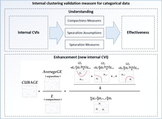
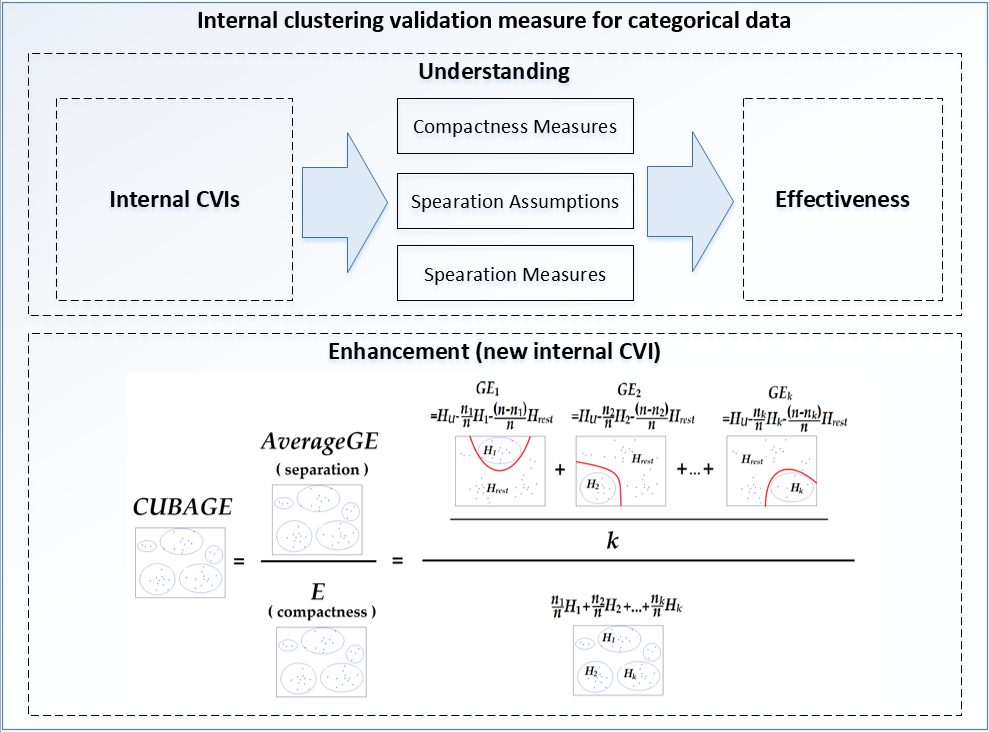
3. Understanding of Internal Clustering Validation Indexes

In this section, we theoretically analyzed the effectiveness of the clustering validity evaluation of the five internal CVIs mentioned above, i.e., the entropy function (E), the k-modes objective function (F), the CLOPE objective function (Clope_r), the averaged category utility function (CU_1/k), and the CDCS objective function (R). We pointed out the compactness measure and the separation measures (assumptions) of them. We also analyzed the ineffectiveness of using compactness alone in clustering validation measurement.

3.1. Generalization and an Example

To better understand the composition of the CVIs, we first generalized them into

Table 1. Summary of the aforementioned clustering validation indexes (CVIs).

CVI	Compactness Core	$\mathbf{Average}\mathbf{Compactness}\left(\overline{\mathit{C}\mathit{o}\mathit{m}}\right)$	Objective
E(P)	$-{\displaystyle \sum _{j=1}^m{\displaystyle \sum _{i=1}^{d_j}p(a_j{}^{(i)}|C_l)\log (p(a_j{}^{(i)}|C_l))}}$	${\displaystyle \sum _{l=1}^{k}p(C_l)}\cdot Core$	$\begin{array}{cc}Minimize& \overline{Com}\end{array}$
F(P)	${\displaystyle \sum _{j=1}^m[(1-{\max }_{i=1}^{d_j}p(a_j{}^{(i)}|C_l)]}$	${\displaystyle \sum _{l=1}^{k}p(C_l)}\cdot Core$	$\begin{array}{cc}Minimize& n\cdot \overline{Com}\end{array}$ *
Cloper(P)	${[{\displaystyle \sum _{j=1}^m\left|D(A_j|C_l)\right|}]}^{-r}$	${\displaystyle \sum _{l=1}^{k}p{(C_l)}^2}\cdot Core$	$\begin{array}{cc}Maximize& n\cdot m\cdot \overline{Com}\end{array}$ *
CU1/k(P)	${\displaystyle \sum _{j=1}^m{\displaystyle \sum _{i=1}^{d_j}p{(a_j{}^{(i)}|C_l)}^2}}-Constant$	${\displaystyle \sum _{l=1}^{k}p(C_l)}\cdot Core$	$\begin{array}{cc}Maximize& k^{-1}\cdot \overline{Com}\end{array}$
R(P)	${\displaystyle \sum _{j=1}^m{[{\max }_{i=1}^{d_j}p(a_j{}^{(i)}|C_l)]}^3}$	${\displaystyle \sum _{l=1}^{k}p(C_l)}\cdot Core$	$\begin{array}{cc}Maximize& m^{-1}\cdot \overline{Com}\cdot inter{(P)}^{-1}\end{array}$ *

* Note that the number attributes m and the number of objects n are invariable to any partition.

. The compactness cores use intra-cluster information to measure the compactness of each cluster based on the consensus that the attribute values in a compact cluster should be concentrated. As shown in Table 1, all five CVIs can evolve the compactness measure with different cores.

We addressed our concerns about the effectiveness of these CIVs with an example.

Table 2. Example of a dataset with five partitions. The number of clusters is 2, 3, 4, 5, and 6, respectively.

Object	A1	A2	A3	Partition 1	Partition 2	Partition 3	Partition 4	Partition 5
X1	a	d	h	1	1	1	1	1
X2	a	e	i	1	1	1	1	1
X3	a	f	h	1	1	1	2	2
X4	b	g	h	1	2	2	3	3
X5	b	g	h	1	2	2	3	4
X6	b	f	h	1	2	3	4	5
X7	c	d	j	2	3	4	5	6

is an example of a dataset and five partitions of it. We evaluated these five partitions with E, F, Clope_1~3, CU_1/k, and R, respectively; the results are shown in

Table 3. Evaluation results of the partitions in Table 2.

CVI	Partition 1	Partition 2	Partition 3	Partition 4	Partition 5
E(P) *	2.120	1.016	0.744	0.396	0.396
F(P) *	8	4	3	2	2
Clope1(P)	2.071	1.750	1.500	1.343	1.057
Clope2(P)	0.289	0.396	0.393	0.402	0.307
Clope3(P)	0.046	0.094	0.113	0.125	0.093
CU1/k(P)	0.255	0.376	0.330	0.302	0.252
R(P)	47.353	29.321	20.652	14.844	8.019

* To optimize E and F is to minimize them, while other functions are to be maximized.

, the optimal scores of each CVI are bolded.

In Table 3, the bolded values are the optimal values measured by each index. As we can see, the opinions of different CVIs did not agree, and as the number of clusters increased, the values of E, F, Clope₁, and R, monotonically decreased. Generally, if the valuation outcome tended to change with the number of clusters monotonically, the evaluation methods may not be suited for comparing partitions of different cluster numbers, since they will bias towards choosing the partition of less or more clusters. We start our discussion on the effectiveness of E and F—the CVIs showed monotonicity, and only use compactness measures.

3.2. Analysis of Indexes E and F

The indexes E and F use compactness measures only, and average the compactness by a weight that was linear to the cluster size p(C_l). We can show that the values of index E and F are monotonic to the number of clusters when clustering hierarchically:

Theorem 1.

Given dataset U, described by a set of independent attributes V = {A₁, …, A_m}, P₁ and P₂ are two partitions of U. If P₁ = {C₁, …, C_k} and P₂ = {C₁, …, C_k-1, C_s1, …, C_st}, where C_k = C_s1 ∪ C_s2 ∪ …∪ C_st, C_sl ≠ Φ, and C_sl ∩ C_sl’ = Φ (l ≠ l’; l, l’ = 1, …, t), then E(P₁) ≥ E(P₂), and the equality holds if and only if p(V|C_s1) = p(V|C_s2) = … = p(V|C_st).

Proof of Theorem 1.

According to Equations (2) and (3), we know that:

$$\{\begin{array}{l}E(P_1)=-{\displaystyle \sum _{j=1}^m{\displaystyle \sum _{l=1}^{k-1}p(C_l){\displaystyle \sum _{i=1}^{d_j}p(a_j{}^{(i)}|C_l)\log (p(a_j{}^{(i)}|C_l))}}}-{\displaystyle \sum _{j=1}^{m}p(C_k){\displaystyle \sum _{i=1}^{d_j}p(a_j{}^{(i)}|C_k)\log (p(a_j{}^{(i)}|C_k))}},\\ E(P_2)=-{\displaystyle \sum _{j=1}^m{\displaystyle \sum _{l=1}^{k-1}p(C_l){\displaystyle \sum _{i=1}^{d_j}p(a_j{}^{(i)}|C_l)\log (p(a_j{}^{(i)}|C_l))}}}-{\displaystyle \sum _{j=1}^m{\displaystyle \sum _{l=1}^{t}p(C_{sl}){\displaystyle \sum _{i=1}^{d_j}p(a_j{}^{(i)}|C_{sl})\log (p(a_j{}^{(i)}|C_{sl}))}}}.\end{array}$$

Then:

$$E(P_1)-E(P_2)={\displaystyle \sum _{j=1}^m[{\displaystyle \sum _{l=1}^{t}p(C_{sl}){\displaystyle \sum _{i=1}^{d_j}p(a_j{}^{(i)}|C_{sl})\log (p(a_j{}^{(i)}|C_{sl}))}}-p(C_k){\displaystyle \sum _{i=1}^{d_j}p(a_j{}^{(i)}|C_k)\log (p(a_j{}^{(i)}|C_k))}]}.$$

(19)

Therefore, the necessary and sufficient condition of E(P₁) ≥ E(P₂) is:

$$-{\displaystyle \sum _{j=1}^{m}p(C_k){\displaystyle \sum _{i=1}^{d_j}p(a_j{}^{(i)}|C_k)\log (p(a_j{}^{(i)}|C_k)}})\ge -{\displaystyle \sum _{j=1}^m{\displaystyle \sum _{l=1}^t\frac{p(C_{sl})}{p(C_k)}{\displaystyle \sum _{i=1}^{d_j}p(a_j{}^{(i)}|C_{sl})\log (p(a_j{}^{(i)}|C_{sl})}}}),$$

(20)

Since C_s1 ∪ C_s2 ∪ … ∪ C_st = C_k, C_sl ≠ Φ, and C_sl ∩ C_sl’ = Φ (l ≠ l’; l, l’ = 1, …, t), we can show that:

$$\begin{array}{cc}{\displaystyle \sum _{l=1}^t\frac{p(C_{sl})}{p(C_k)}}={\displaystyle \sum _{l=1}^{t}p(C_{sl}|C_k)=1,}& l=1,...,t\end{array}.$$

(21)

Meanwhile, due to Bayes’ theorem, we can establish that:

$$\begin{array}{cc}\hfill {\displaystyle \sum _{l=1}^t\frac{p(C_{sl})}{p(C_k)}p(a_j{}^{(i)}|C_{sl})}& ={\displaystyle \sum _{l=1}^t\frac{p(C_{sl})}{p(C_k)}\cdot \frac{p(a_j{}^{(i)})\cdot p(C_{sl}|a_j{}^{(i)})}{p(C_{sl})}}\hfill \\ & ={\displaystyle \sum _{l=1}^t\frac{1}{p(C_k)}\cdot p(a_j{}^{(i)})\cdot p(C_{sl}|a_j{}^{(i)})}\hfill \\ & =\frac{p(C_k|a_j{}^{(i)})}{p(C_k)}\cdot p(a_j{}^{(i)})\hfill \\ & =p(a_j{}^{(i)}|C_k),\hspace{1em}i=1,...,d_j,\hspace{1em}j=1,...,m\hfill \end{array}$$

(22)

Since the attributes are independent, and we know that H(X) is a concave function, we can prove Inequality (20) to be true by Jensen’s inequality [51].

Also, H(X) is not linear. Due to Jensen’s inequality, the equality holds if and only if p(a_j⁽ⁱ⁾|C_s1) = p(a_j⁽ⁱ⁾|C_s2) = … = p(a_j⁽ⁱ⁾|C_st) (j = 1, …, m; i = 1, …, d_j), which is p(V|C_s1) = p(V|C_s2) = … = p(V|C_st). □

Theorem 2.

If the conditions are the same as in Theorem 1, then F(P₁) ≥ F(P₂), and the equality holds if and only if z_1j = z_2j = … = z_tj (j = 1, …, m), where z_lj is the mode of the values of attribute A_j in cluster C_sl (l = 1, …, t).

Proof of Theorem 2.

Similar to the proof of Theorem 1, we can show that:

$$F(P_1)-F(P_2)=d_{cluster}(C_k)-{\displaystyle \sum _{l=1}^t{d}_{cluster}(C_{sl})}={\displaystyle \sum _{j=1}^m{\displaystyle \sum _{i=1}^{\left|C_k\right|}\delta (x_{kij},z_{kj})-}}{\displaystyle \sum _{l=1}^t{\displaystyle \sum _{j=1}^m{\displaystyle \sum _{i=1}^{\left|C_{sl}\right|}\delta (x_{lij},z_{lj})}}}.$$

(23)

Since C_s1 ∪ C_s2 ∪ … ∪ C_st = C_k, C_sl ≠ Φ, and C_sl ∩ C_sl’ = Φ (l ≠ l’; l, l’ = 1, …, t), to any attribute A_j, the occurrence of value a_j⁽ⁱ⁾ in cluster C_k is equal to the sum of the occurrence of the same value in cluster C_s1 to C_st:

$$\begin{array}{cc}\begin{array}{cc}Occ(a_j{}^{(i)},C_k)={\displaystyle \sum _{l=1}^{t}Occ(a_j{}^{(i)},C_{sl})},& j=1,\dots ,m,\end{array}& i=1,...,d_j\end{array}.$$

(24)

Meanwhile, we can rewrite the dissimilarity of any cluster C_q of dataset U as:

$$d_{cluster}(C_q)={\displaystyle \sum _j^m[|C_q|-Occ(z_{qj},C_q)]}.$$

(25)

Applying Equation (25) to Equation (23) yields:

$$F(P_1)-F(P_2)={\displaystyle \sum _j^m[|C_k|-Occ(z_{kj},C_k)]}-{\displaystyle \sum _{l=1}^t{\displaystyle \sum _j^m[|C_{sl}|-Occ(z_{lj},C_{sl})]}}.$$

(26)

By the definition of mode, we know that:

$$Occ(z_{lj},C_{sl})\ge Occ(z_{kj},C_{sl}), j=1,\dots ,m, l=1,...,t.$$

(27)

Then:

$${\displaystyle \sum _{l=1}^t{\displaystyle \sum _j^m[|C_{sl}|-Occ(z_{lj},C_{sl})]}}\le {\displaystyle \sum _{l=1}^t{\displaystyle \sum _j^m[|C_{sl}|-Occ(z_{kj},C_{sl})]}}.$$

(28)

Therefore:

$$F(P_1)-F(P_2)\ge {\displaystyle \sum _j^m[|C_k|-Occ(z_{kj},C_k)]}-{\displaystyle \sum _{l=1}^t{\displaystyle \sum _j^m[|C_{sl}|-Occ(z_{kj},C_{sl})]}}.$$

(29)

By Equation (24), we can show that the right-hand part of Inequality (29) equals 0. Therefore, F(P₁) ≥ F(P₂), and the equality holds if and only if:

$$Occ(z_{lj},C_{sl})=Occ(z_{kj},C_{sl}), j=1,\dots ,m, l=1,...,t.$$

(30)

□

Theorems 1 and 2 show that one cannot determine whether any clusters in the partition should be merged by E or F, since the evaluation results always suggest to divide. Even if the attribute distribution in the candidate clusters are equivalent (in which case they are generally regarded as the most similar clusters), the scores of whether to merge them would be in a tie. This most affects the hierarchical clustering, in which objects are clustered in either agglomerative or divisive manners, and the suggested layer of hierarchy by these CVIs would always be the layer with the most clusters, unless the layer with the second-most clusters has the same evaluation score.

We should point out that, in some researches, the separation coefficient 1/k of index CU_1/k (which will be discussed shortly) was multiplied to the function E(P) directly, which would aggravate the monotonicity, since 1/k is also a monotonically decreasing function with respect to the partition size. Therefore, we will not discuss such a method in this paper.

3.3. Analysis of Indexes CU_1/k, Clope_r, and R

Besides the compactness measure, indexes CU_1/k, Clope_r, and R use separation measures or assumptions as well. CU_1/k(P) is the averaged compactness over k clusters weighted by p(C_l), and CU_1/k(P) is the further averaged CU(P). The role of the multiplicand 1/k is a crude overfitting control, and can be regarded as the assumed separation coefficient with respect to the number of clusters. We can show that the compactness measure in CU_1/k(P) also shows monotonicity in the previous scenario:

Theorem 3.

If the conditions are the same as in Theorem 1, then CU(P₁) ≤ CU(P₂), and the equality holds if and only if p(V|C_s1) = p(V|C_s2) = … = p(V|C_st).

Proof of Theorem 3.

Similar to the proof of Theorem 1, we can show that:

$$CU(P_1)-CU(P_2)={\displaystyle \sum _{j=1}^m[p(C_k){\displaystyle \sum _{i=1}^{d_j}p{(a_j{}^{(i)}|C_k)}^2}-{\displaystyle \sum _{l=1}^{t}p(C_{sl}){\displaystyle \sum _{i=1}^{d_j}p{(a_j{}^{(i)}|C_{sl})}^2)}}]}.$$

(31)

C_k ≠ Φ, so we can rewrite Equation (31) as:

$$\frac{CU(P_1)-CU(P_2)}{p(C_k)}={\displaystyle \sum _{j=1}^m[{\displaystyle \sum _{i=1}^{d_j}p{(a_j{}^{(i)}|C_k)}^2}-{\displaystyle \sum _{l=1}^t\frac{p(C_{sl})}{p(C_k)}{\displaystyle \sum _{i=1}^{d_j}p{(a_j{}^{(i)}|C_{sl})}^2)}}]}.$$

(32)

Therefore, the necessary and sufficient condition of CU(P₁) ≤ CU(P₂) is:

$$p{(a_j{}^{(i)}|C_k)}^2\le {\displaystyle \sum _{l=1}^t\frac{p(C_{sl})}{p(C_k)}p{(a_j{}^{(i)}|C_{sl})}^2,} i=1,...,d_j, j=1,...,m.$$

(33)

We know that y = x² is a convex, and not a linear function. Therefore, Inequality (33) is true, due to Jensen’s inequality with Equations (21) and (22) in the proof of Theorem 1, and the equality holds if and only if p(V|C_s1) = p(V|C_s2) = … = p(V|C_st). □

Therefore, using the category utility function to evaluate partitions of different size without the separation coefficient 1/k is questionable. However, the act of multiplying the compactness with such a coefficient is based on the assumption that the separation of the partition is negatively correlated with the partition size. Such an assumption ignores the attribute value distribution between clusters, and may generate a new bias to the partitions of fewer clusters, since 1/k would be dominant to the result when the change in compactness is relatively gradual.

The compactness core of Clope_r(P) is also monotonic. However, different to other indexes, Clope_r(P) uses the quadratic weight p(C_l)² instead of p(C_l) to average the compactness. In consequence, the partitions in which the objects are more concentrated in fewer clusters would score better with Clope_r(P), which is also an assumption of separation for adjusting the evaluation results. Like the separation coefficient 1/k of CU_1/k(P), such an assumption is irrelevant to the differences in attribute values between clusters. If we remove the assumption, i.e., we use p(C_l) instead of p(C_l)², the averaged compactness would also be monotonic to the partition size in the previous scenario:

Theorem 4.

If the conditions are the same as in Theorem 1, and we have the compactness measure as followed:

$$G(P)=n\cdot m\cdot {\displaystyle \sum _{l=1}^{k}p(C_l)\cdot {[{\displaystyle \sum _{j=1}^m\left|D(A_j|C_l)\right|}]}^{-r}},$$

(34)

where r is a parameter greater than zero, then G(P₁) ≤ G(P₂), and the equality holds if and only if D(A_j|C_k) = D(A_j|C_s1) = D(A_j|C_s2) =… = D(A_j|C_st), (j = 1, …, m).

Proof of Theorem 4.

Similar to the proof of Theorem 1, we can show that:

$$\frac{G(P_1)-G(P_2)}{n\cdot m}={\displaystyle \sum _{j=1}^m\left[p(C_k)\cdot {\left|D(A_j|C_k)\right|}^{-r}-{\displaystyle \sum _{l=1}^{t}p(C_{sl})\cdot {\left|D(A_j|C_{sl})\right|}^{-r}}\right]},$$

(35)

Since C_s1 ∪ C_s2 ∪ … ∪ C_st = C_k, C_sl ≠ Φ, and C_sl ∩ C_sl’ = Φ (l ≠ l’; l, l’ = 1, …, t), to any attribute A_j:

$$\{\begin{array}{l}p(C_k)={\displaystyle \sum _{l=1}^{t}p(C_{sl}),}\\ {\left|D(A_j|C_k)\right|}^{-r}\le {\left|D(A_j|C_{sl})\right|}^{-r},\hspace{1em}r>0,\hspace{1em}j=1,...m,\hspace{1em}l=1,...t.\end{array}$$

(36)

Therefore, the value of Equation (35) is not greater than zero, the equality holds if and only if |D(A_j|C_k)| = |D(A_j|C_s1)| = |D(A_j|C_s2)| = … = |D(A_j|C_st)|, (j = 1, …, m), which is equal to D(A_j|C_k) = D(A_j|C_s1) = D(A_j|C_s2) = … = D(A_j|C_st), (j = 1, …, m). □

To look more deeply, the essential effect of parameter r in Clope_r(P) is the subjectively adjusted trade-off between compactness and separation (assumption). The compactness would be less important in the evaluation as the value of r decreases, and it would be entirely ignored when r = 0 (although it is avoided). As a result, in Table 3, Clope₂(P) and Clope₃(P) choose the partition with more clusters, due to the effect of compactness, and Clope₁(P) chooses the partition of least clusters, due to the effect of the separation assumption. Therefore, setting r is actually setting the preference for compactness or separation, and could be unfounded in the unsupervised scenario.

The compactness measure of index R is also monotonic to the partition size, since maximizing the compactness of R(P) can be easily proven to be equivalent to minimizing the function F(P). The separation measure of R(P) evaluates the inter-cluster similarity Sim(C_t, C_s) pairwise. The compactness and the separation of R(P) only considers the most and least common values, respectively, which might lower the sensitivity to the value distribution. We will test and discuss the effectiveness of such methods in the experimental section.

4. Internal Clustering Validation Index: CUBAGE

As discussed previously, the CVIs cannot effectively evaluate the partitions of different sizes if the separation measures or assumptions are absent, and the crude separation assumptions without respect to the attribute values are rather questionable.

In this section, we first proposed a new method to measure the inter-cluster separation. Then, we present our algorithm to internally measure the clustering validation, namely, the clustering utility based on the averaged information gain of isolating each cluster (CUBAGE).

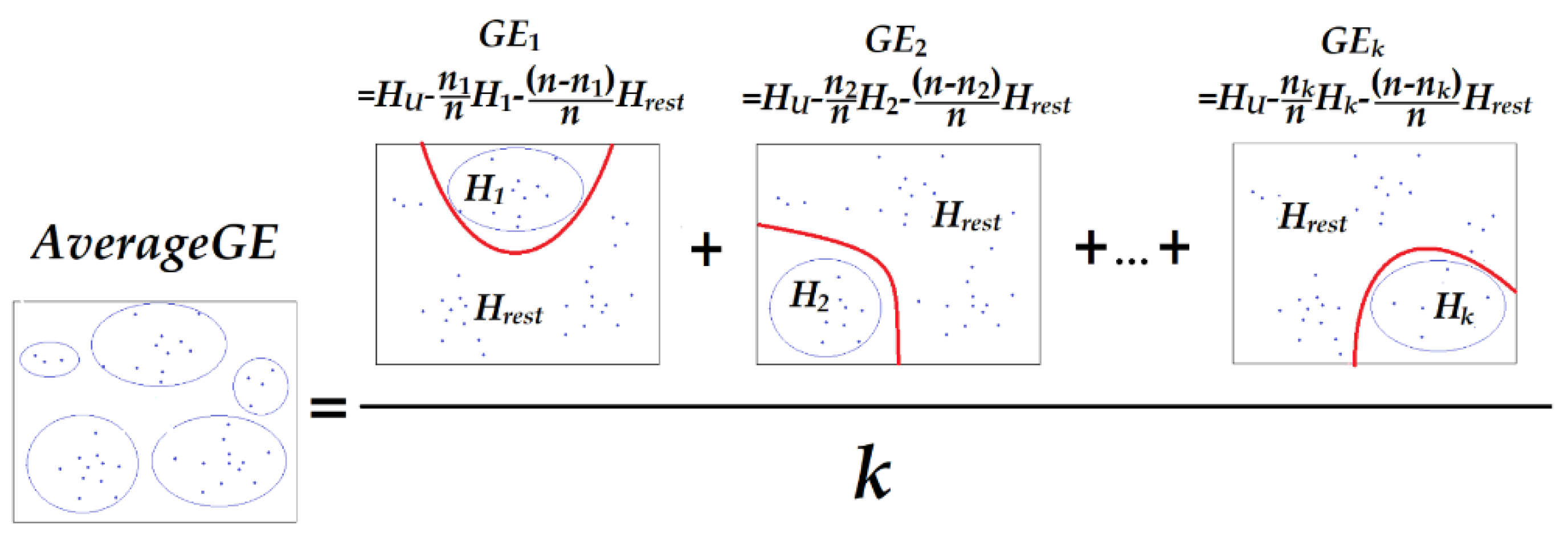
4.1. Inter-Cluster Separation Measure: AGE

Our measure of inter-cluster separation—averaged information gain of isolating each cluster, henceforth AGE—was based on the idea of information gain in information theory. Before presenting AGE, we will review the concept of information gain.

The mutual information is a measure of the shared information of two discrete variables X and Y [52]:

$$I(X;Y)=H(X)-H(X|Y)={\displaystyle \sum _{y\in Y}{\displaystyle \sum _{x\in X}p(x,y)\log (\frac{p(x,y)}{p(x)p(y)})}}.$$

(37)

In machine learning, the mutual information I(X; Y) is the expected information gain; that is, the reduction in the entropy of X that is achieved by learning the state of Y [53]. In general terms, the expected information gain is the change in entropy from a prior state (X) to a state that takes some information (X|Y):

$$IG(X,Y)=H(X)-H(X|Y).$$

(38)

Given a partition P = {C_l} (l = 1, …, k) of dataset U, which is described by V = {A₁, …, A_m}, we define the information gain of separating cluster C_l from other clusters as:

$$GE(C_l)=H(V)-H(V|P_l),$$

(39)

where P_l= {C_l, U − C_l} is the partition that separates C_l from other clusters, and U − C_l is the complementary set of C_l.

GE(C_l) is the information gain of V from the unpartitioned state to the state where the objects are divided into C_l and U − C_l; in other words, the degree of certainty that we can gain by separating the objects in C_l from other objects. Therefore, GE(C_l) equals the dissimilarity between C_l and other clusters (U − C_l); a higher value of GE(C_l) indicates that more separation is achieved by separating C_l with other clusters.

As Figure 2 illustrates, we average the value of GE over all the scenarios of isolating each cluster to measure the overall separation:

$$AGE(P)=\frac{1}{k}{\displaystyle \sum _l^{k}GE(C_l)}=\frac{1}{k}{\displaystyle \sum _l^k[H(V)-H(V|P_l)}].$$

(40)

Explicitly, AGE(P) is calculated as:

$$AGE(P)=\frac{1}{k}{\displaystyle \sum _l^k[H(V)-p(C_l)\cdot H(V_{C_l})-p(U-C_l)\cdot H(V_{U-C_l})]},$$

(41)

where $V_{C_l}$ is the set of attributes describing the objects in C_l, $V_{U-C_l}$ is the set of attributes describing other objects, and:

$$\{\begin{array}{l}H(V)=-{\displaystyle \sum _{j=1}^m{\displaystyle \sum _{i=1}^{d_j}p(a_j{}^{(i)})\log (p(a_j{}^{(i)}))}},\\ H(V_{C_l})=-{\displaystyle \sum _{j=1}^m{\displaystyle \sum _{i=1}^{d_j}p(a_j{}^{(i)}|C_l)\log (p(a_j{}^{(i)}|C_l))}},\\ H(V_{U-C_l})=-{\displaystyle \sum _{j=1}^m{\displaystyle \sum _{i=1}^{d_j}p(a_j{}^{(i)}|U-C_l)\log (p(a_j{}^{(i)}|U-C_l))}}.\end{array}$$

(42)

4.2. Upper and Lower Bounds of AGE

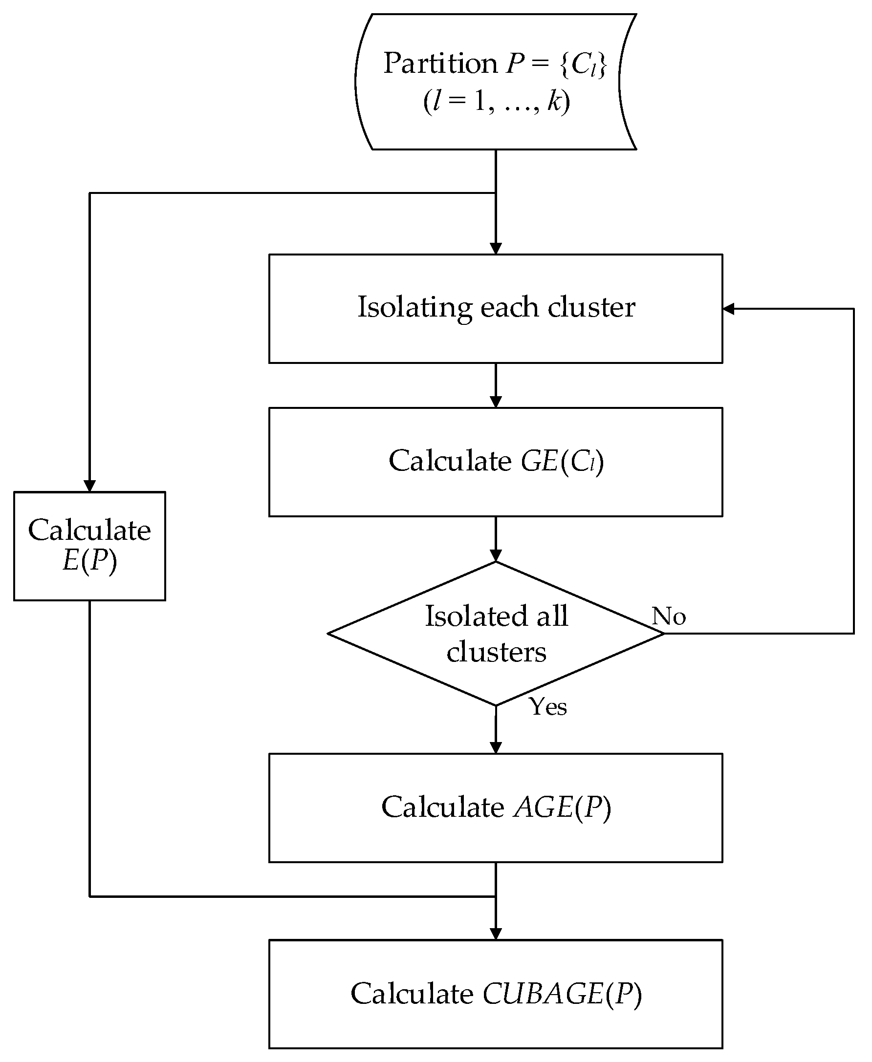
By the property of information gain, the lower bound of AGE(P) is zero:

$$AGE(P)\ge 0.$$

(43)

We will discuss the upper bound respectively:

1. When the number of clusters k ≤ 2:

$$\begin{array}{cc}AGE(P)=\frac{1}{k}{\displaystyle \sum _l^k[H(V)-E(P_l)}]=H(V)-E(P),& k\le 2.\end{array}$$

(44)

This indicates that for a given dataset, maximizing AGE(P) is equivalent to minimizing E(P) when the size of the partition is no greater than 2. This is because that the whole partition is affirmatory when one of the clusters is learned. Moreover, when the objects are not separated at all, i.e., k = 1, the value of AGE(P) is 0;

2. When the number of clusters k > 2, due to Theorem 1, we can establish that:

$$\begin{array}{cc}AGE(P)=\frac{1}{k}{\displaystyle \sum _l^k[H(V)-E(P_l)}]\le \frac{1}{k}{\displaystyle \sum _l^k[H(V)-E(P)}]=H(V)-E(P),& k>2.\end{array}$$

(45)

The equality of Inequality (45) holds if and only if the attribute value distributions in each cluster are all the same, under which circumstances the value of E(P) would be equal to H(V); therefore, AGE(P) = 0.

To sum up, the upper bound of AGE(P) is H(V) − E(P) and the lower bound is 0. The value of the upper bound becomes equal with the lower bound 0 when the objects are not separated at all, or the attribute value distributions in each cluster are all the same; this means that the AGE(P) yields the minimum possible value when the objects are least separated.

4.3. CUBAGE Index

Our internal clustering validation index, CUBAGE, uses AGE(P) as the inter-cluster separation measure, and uses the reciprocal of the conditional entropy, E(P)⁻¹, as the intra-cluster compactness:

$$CUBAGE(P)=Sep(P)*Com(P)=AGE(P)\cdot E{(P)}^{-1}.$$

(46)

This index takes a form of the product of the separation and the compactness. A higher value of CUBAGE(P) indicates a better clustering result. As shown in

Table 4. The AGE (averaged information gain of isolating each cluster) and CUBAGE (clustering utility based on AGE) outcomes of the partitions in Table 2.

CVI	Partition 1	Partition 2	Partition 3	Partition 4	Partition 5
AGE	1.032	1.191	0.912	0.769	0.601
CUBAGE	0.487	1.172	1.226	1.941	1.518

, neither AGE(P) nor CUBAGE(P) showed monotonicity with respect to the partition size.

Additionally, when the size of the partition is no greater than 2, we can establish the following by Equations (44) and (46):

$$\begin{array}{cc}CUBAGE(P)=\frac{\frac{1}{k}{\displaystyle \sum _l^k[H(V)-E(P_l)}]}{E(P)}=\frac{H(V)-E(P)}{E(P)}=\frac{H(V)}{E(P)}-1,& k\le 2.\end{array}$$

(47)

Equation (47) is actually the information gain ratio of the partition. This means that for a given dataset, maximizing CUBAGE(P) is equivalent to minimizing E(P) when the number of clusters is no greater than 2, since the term H(V) is a constant to the dataset.

Given a partition P, the value of CUBAGE(P) can be calculated, as shown in Figure 3. Algorithms 1 and 2 are the pseudocode of CUBAGE.

Algorithm 1 Clustering Utility based on Entropy (CUBAGE)

Input: dataset with n objects: U = (Xi); label of a partition with k clusters; Output: CUBAGE value of the partition; Called Function: entropy calculation function: Entropy(objects); Begin: 1.  Calculate the entropy of the whole dataset, save as HU: HU = Entropy(U); 2.  For each cluster Cl: 3.    Calculate the entropy of objects in Cl, save in vector H:H(l) = Entropy(Cl); 4.    Calculate the entropy of objects in U − Cl, save in vector HC:HC(l) = Entropy(U − Cl); 5.  End for; 6.  Generate weight vector: W = 1/n·[|C1|, | C2|, …, | Cl|]; 7.  Calculate the dot product E = W·H; 8.  Calculate AGE = HU − 1/k·[E + (1 − W)·HC]; Return: 9.  CUBAGE = AGE/E;

The time complexity of CUBAGE(P) is O(kmn), where k is the number of clusters, m is the number of attributes, and n is the total number of objects. Note that there is no extra time cost for computing the compactness E⁻¹(P), since the weighted entropy of each cluster is already calculated during computing the separation AGE(P). The time cost could be lower if the data is sparse. Furthermore, one can easily apply parallel or distributed computing to CUBAGE(P) by the objects or the attributes to reduce the computing time. Therefore, such time complexity makes CUBAGE(P) scalable to large datasets.

Algorithm 2 Entropy calculation function

Input: a set of x objects; Output: Entropy of objects in a single set; Begin: 1.  For each attribute Aj: 2.    Calculate the entropy of the attribute by Equation (1), save in vector HA; 3.  End for; Return: 4.  Entropy = sum(HA);

5. Experiments and Discussion

In this section, we present the results of the comparative experiments to evaluate the effectiveness of CUBAGE, along with the five internal CVIs mentioned above. We used −F(P) and −E(P) instead of F(P) and E(P) to unify the objectives, and maximized each function to search for the local optimal partition.

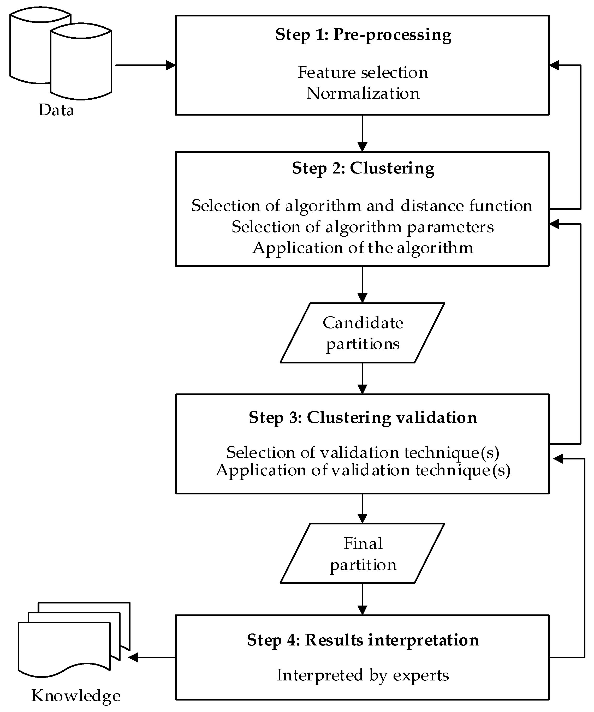
5.1. Experimental Methods

We tested the CVIs on eight datasets from the UCI (University of California, Irvine) Machine Learning Repository (http://archive.ics.uci.edu/mL/index.php), as shown in

Table 5. Datasets from UCI.

Dataset	Objects	Attributes	Classes	Object Distribution
Voting	435	16	2	168, 267
Breast Cancer Wisconsin (Original)	683	9	2	444, 239
Mushroom	5644	22	2	2156, 3488
Soybean (Small)	47	35	4	10, 10, 10, 17
Car Evaluation	1728	6	4	1210, 384, 69, 65
Heart Disease (Cleveland)	297	13	5	54, 35, 35, 13, 160
Dermatology	358	34	6	111, 60, 71, 48, 48, 20
Zoo	101	16	7	41, 20, 5, 13, 4, 8, 10

; records with missing values are removed. To compare the quality of the partitions chosen by the internal CVIs, we used two external CVIs as the benchmark evaluation criteria, respectively:

• The adjusted Rand index (ARI)—the corrected-for-chance version of the Rand index—is based on the numbers of objects in common (or not) between the pre-defined classes and the produced clusters [6]. Given two partitions P = {C₁, …, C_k} and P’ = {C’₁, …, C’_k’} ARI is defined as:

  $$\mathrm{ARI}=\frac{{{\displaystyle \sum }}_{ij}\left(\begin{array}{c}{n}_{ij}\\ 2\end{array}\right)-\left[{{\displaystyle \sum }}_i\left(\begin{array}{c}{b}_i\\ 2\end{array}\right){{\displaystyle \sum }}_j\left(\begin{array}{c}{d}_j\\ 2\end{array}\right)\right]/\left(\begin{array}{c}n\\ 2\end{array}\right)}{\frac{1}{2}\left[{{\displaystyle \sum }}_i\left(\begin{array}{c}{b}_i\\ 2\end{array}\right)+{{\displaystyle \sum }}_j\left(\begin{array}{c}{d}_j\\ 2\end{array}\right)\right]-\left[{{\displaystyle \sum }}_i\left(\begin{array}{c}{b}_i\\ 2\end{array}\right){{\displaystyle \sum }}_j\left(\begin{array}{c}{d}_j\\ 2\end{array}\right)\right]/\left(\begin{array}{c}n\\ 2\end{array}\right)},$$

  (48)

  where n_ij is the number of common objects in C_i and C’_j, n_ij = | C_i ∩ C’_j|, $b_i={\displaystyle \sum }_j{n}_{ij}$, $d_j={\displaystyle \sum }_i{n}_{ij}$.

In a specific dataset, a partition that is more similar to the pre-defined classes would score higher values in ARI. Note that ARI may take negative values.

• The normalized mutual information (NMI) calculates the mutual information of two partitions, and normalizes it with the sum of their entropy [16]:

  $$\mathrm{NMI}=\frac{2{{\displaystyle \sum }}_{i=1}^k{{\displaystyle \sum }}_{j=1}^{k^{\prime }}\frac{n_{ij}}{n}\log \frac{n_{ij}n}{b_i{d}_j}}{-{{\displaystyle \sum }}_{i=1}^k\frac{b_i}{n}\log \frac{b_i}{n}-{{\displaystyle \sum }}_{j=1}^{k^{\prime }}\frac{d_j}{n}\log \frac{d_j}{n}} .$$

  (49)

In a specific dataset, a higher value of NMI indicates that the partition is more proximal to the pre-defined classes.

For example, in one measurement of several partitions, partitions P₁ and P₂ scores best in internal CVIs IV₁ and IV₂, respectively. EV is an external CVI, if EV(P₁) > EV(P₂), we can establish that partition P₁ is more proximal to the pre-defined classes than partition P₂ in the opinion of EV. Therefore, IV₁ performs better than IV₂ in this example.

We first compare the NMI values of the partitions selected by each internal CVIs to find out which internal CVI can select the better partition, i.e., performs better in the opinion of NMI. Then we use ARI to evaluate the internal CVIs in the same manner.

On each dataset, we used the classical agglomerative hierarchical clustering and the k-modes clustering to produce the partitions, and both clustering methods applied the same cluster dissimilarity that was defined in F. The experimental procedures are shown in Figure 4 and Figure 5.

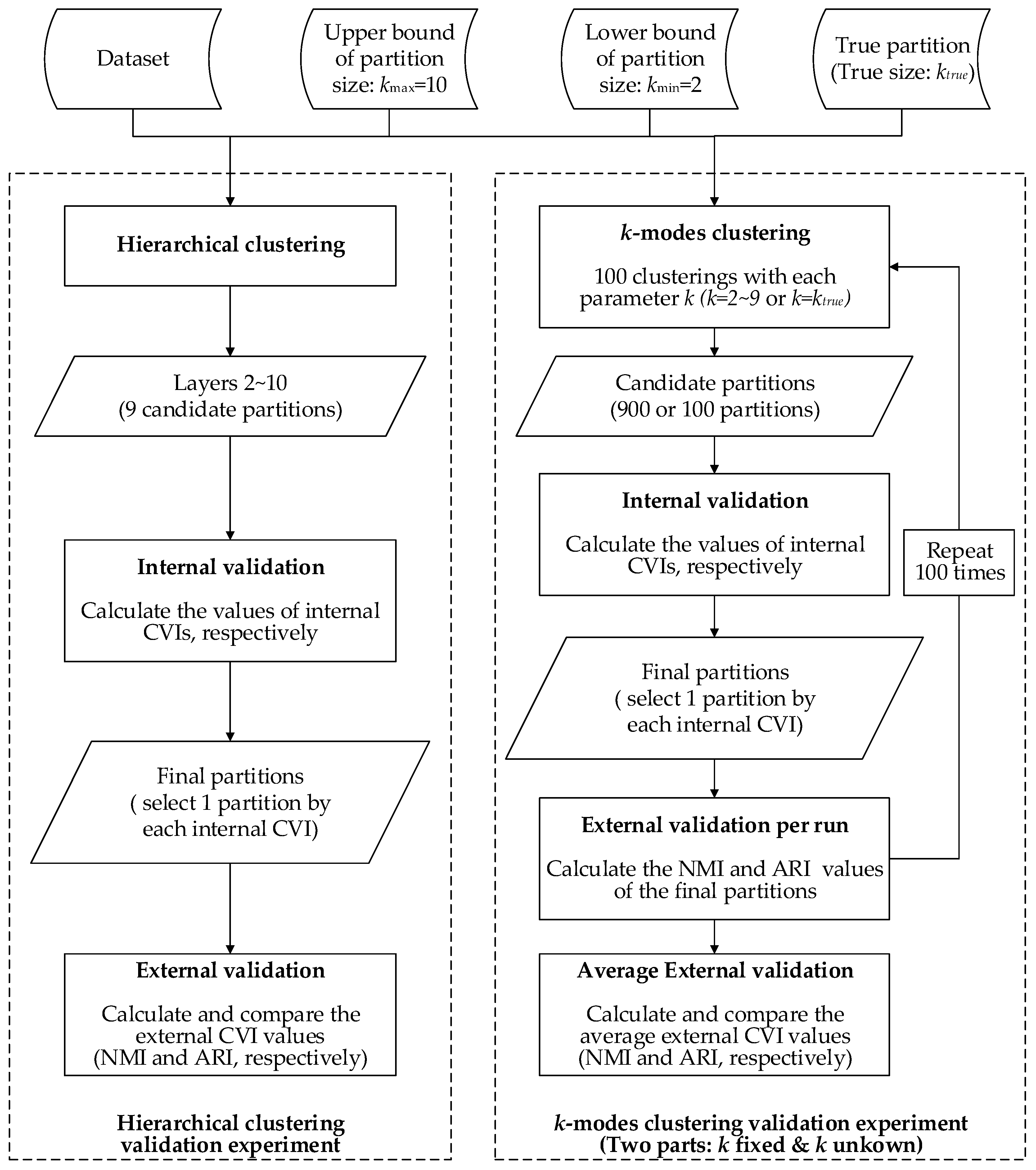
• The agglomerative hierarchical clustering is a ‘bottom-up’ approach; each object is treated as an individual cluster in the beginning. When moving up the hierarchy, pairs of clusters are merged progressively if the dissimilarity of their union is lower than the other pairs in the same layer, until all objects are merged into one cluster eventually. The layers in the hierarchy are different partitions of the dataset. From the generated partitions with the number of clusters ranging from 2–10, we selected one ‘optimal’ partition by each internal CVI, then compared the external CVI values (NMI and ARI, respectively) of the selected partitions.
• The k-modes clustering is a partitioning approach that is similar to the more famous k-means clustering. It starts with k randomly-generated cluster centers (seeds), and each object is assigned to the most appropriate cluster if the dissimilarity of their union is the lowest. In the next iteration, the centers of the clusters are updated by the attribute modes, and the objects are reassigned in the previous manner. The iteration ends if the value of the objective function F stabilizes. The clustering results are inconsistent over different seeds, even if the number of clusters k is fixed. To test the performances when the number of clusters is unknown, we used the internal CVIs to search for the optimal partition from all the partitions produced by k-modes with k ranging from 2–10 (each value of k is conducted 100 times, therefore 900 candidate partitions generated). We further repeated the process 100 times and compared the average external CVI values (ARI and NMI, respectively) of the partitions selected by each internal CVI. Additionally, we tested the internal CVIs with k set to the pre-defined number of clusters to examine the performance when the number of clusters is determined.

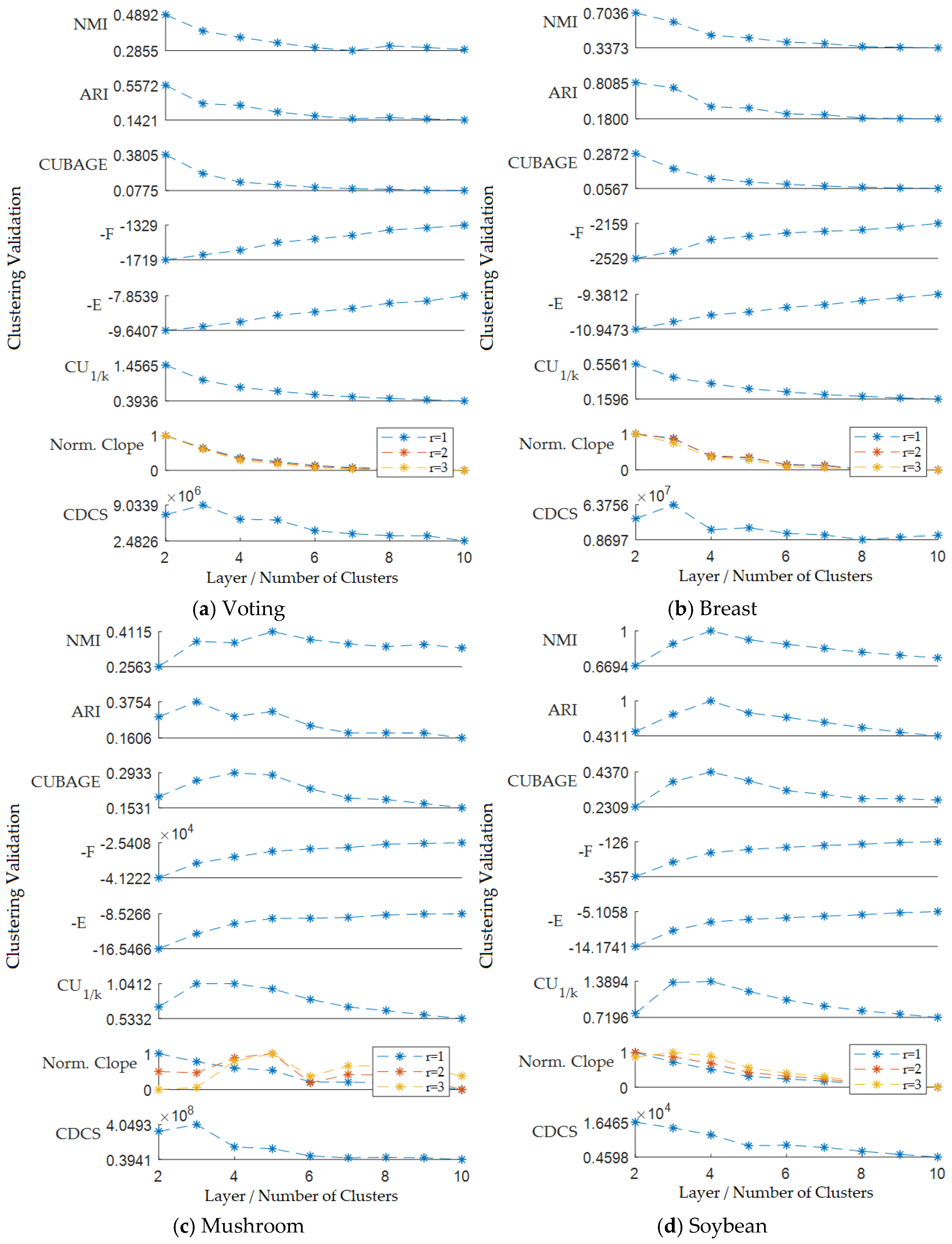
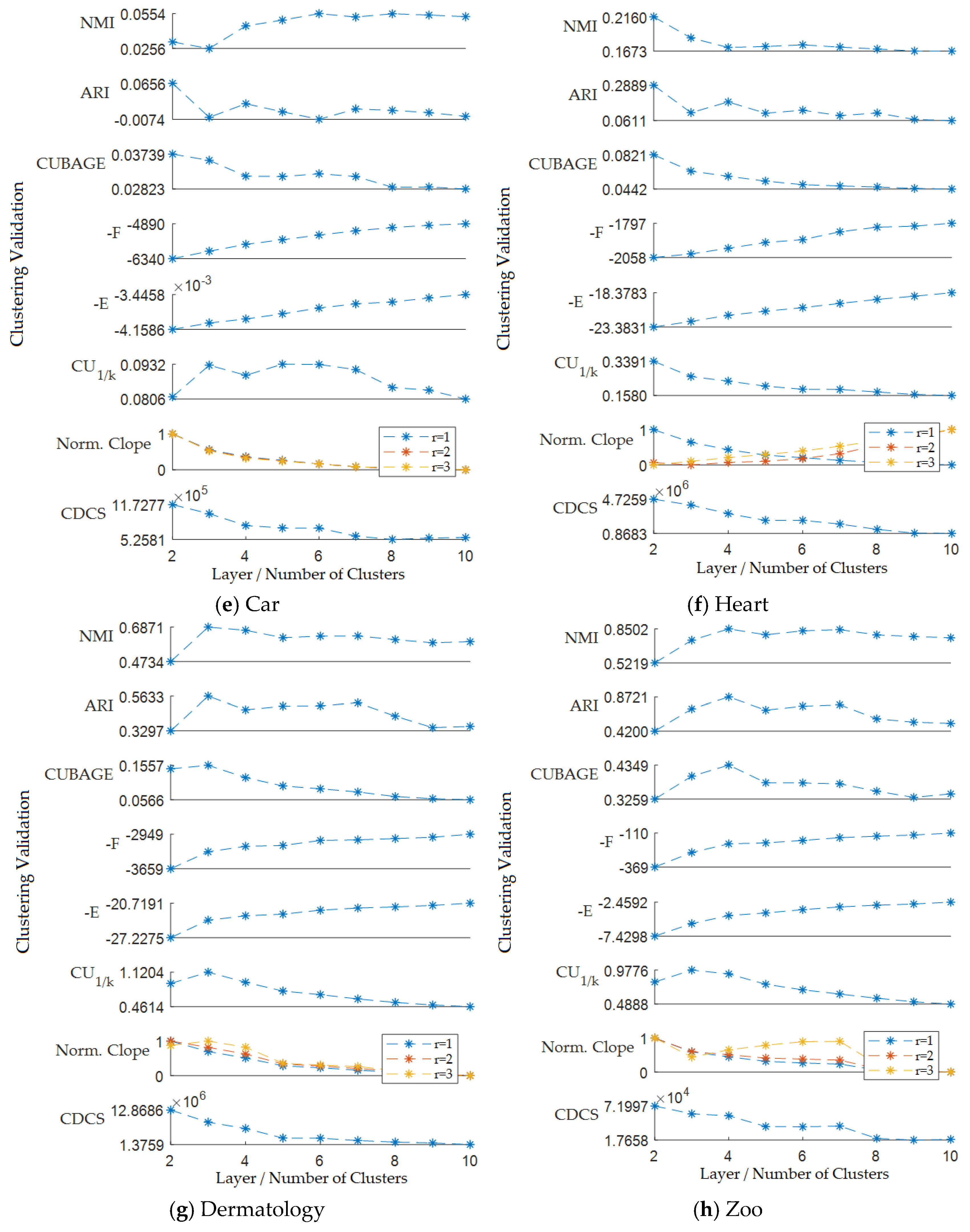
5.2. Results of the Hierarchical Clustering Validation Evaluation

The NMI and ARI scores of the partitions chosen by each internal CVI in the hierarchical clustering are shown in

Table 6. Normalized mutual information (NMI) values of the hierarchical partitions chosen from layers 2–10 by each internal CVI.

Dataset	CUBAGE	−F	−E	CU1/k	Clope1	Clope2	Clope3	R
Voting	(1) 0.489	(7) 0.292	(7) 0.292	(1) 0.489	(1) 0.489	(1) 0.489	(1) 0.489	(6) 0.396
Breast	(1) 0.704	(7) 0.337	(7) 0.337	(1) 0.704	(1) 0.704	(1) 0.704	(1) 0.704	(6) 0.609
Mushroom	(5) 0.362	(6) 0.339	(6) 0.339	(3) 0.368	(8) 0.256	(1) 0.412	(1) 0.412	(3) 0.368
Soybean	(1) 1	(4) 0.745	(4) 0.745	(1) 1	(6) 0.669	(6) 0.669	(3) 0.878	(6) 0.669
Car	(4) 0.031	(1) 0.053	(1) 0.053	(3) 0.05	(4) 0.031	(4) 0.031	(4) 0.031	(4) 0.031
Heart	(1) 0.216	(5) 0.167	(5) 0.167	(1) 0.216	(1) 0.216	(5) 0.167	(5) 0.167	(1) 0.216
Dermatology	(1) 0.687	(4) 0.597	(4) 0.597	(1) 0.687	(6) 0.473	(6) 0.473	(1) 0.687	(6) 0.473
Zoo	(1) 0.85	(2) 0.764	(2) 0.764	(4) 0.741	(5) 0.522	(5) 0.522	(5) 0.522	(5) 0.522
Average NMI *	0.542	0.412	0.412	0.532	0.42	0.433	0.486	0.411
Average Rank *	1.875	4.5	4.5	1.875	4	3.625	2.625	4.625

* Averaged over datasets (average values of each column).

and

Table 7. Adjusted Rand index (ARI) values of the hierarchical partitions chosen from layers 2–10 by each internal CVI.

Dataset	CUBAGE	−F	−E	CU1/k	Clope1	Clope2	Clope3	R
Voting	(1) 0.557	(7) 0.142	(7) 0.142	(1) 0.557	(1) 0.557	(1) 0.557	(1) 0.557	(6) 0.337
Breast	(1) 0.808	(7) 0.18	(7) 0.18	(1) 0.808	(1) 0.808	(1) 0.808	(1) 0.808	(6) 0.72
Mushroom	(5) 0.288	(7) 0.161	(7) 0.161	(1) 0.375	(6) 0.286	(3) 0.318	(3) 0.318	(1) 0.375
Soybean	(1) 1	(7) 0.431	(7) 0.431	(1) 1	(4) 0.501	(4) 0.501	(3) 0.781	(4) 0.501
Car	(1) 0.066	(7) −0.002	(7) −0.002	(6) 0.008	(1) 0.066	(1) 0.066	(1) 0.066	(1) 0.066
Heart	(1) 0.289	(5) 0.061	(5) 0.061	(1) 0.289	(1) 0.289	(5) 0.061	(5) 0.061	(1) 0.289
Dermatology	(1) 0.563	(4) 0.359	(4) 0.359	(1) 0.563	(6) 0.33	(6) 0.33	(1) 0.563	(6) 0.33
Zoo	(1) 0.872	(3) 0.522	(3) 0.522	(2) 0.715	(5) 0.42	(5) 0.42	(5) 0.42	(5) 0.42
Average ARI *	0.555	0.232	0.232	0.539	0.407	0.383	0.447	0.38
Average Rank *	1.5	5.875	5.875	1.75	3.125	3.25	2.5	3.75

* Averaged over datasets (average values of each column).

; the bracketed figures are the performance ranks over indexes. In general, the indexes CUBAGE and CU_1/k performed the best when evaluating the layers of the hierarchical clustering. The results of indexes −F and −E were worse than other indexes in both NMI and ARI. Figure 6 illustrates the changing of validation scores over the layers of the hierarchy; as we can see, the indexes CUBAGE and CU_1/k matched the benchmark evaluation criteria the best.

5.3. Results of the k-Modes Clustering Validation Evaluation

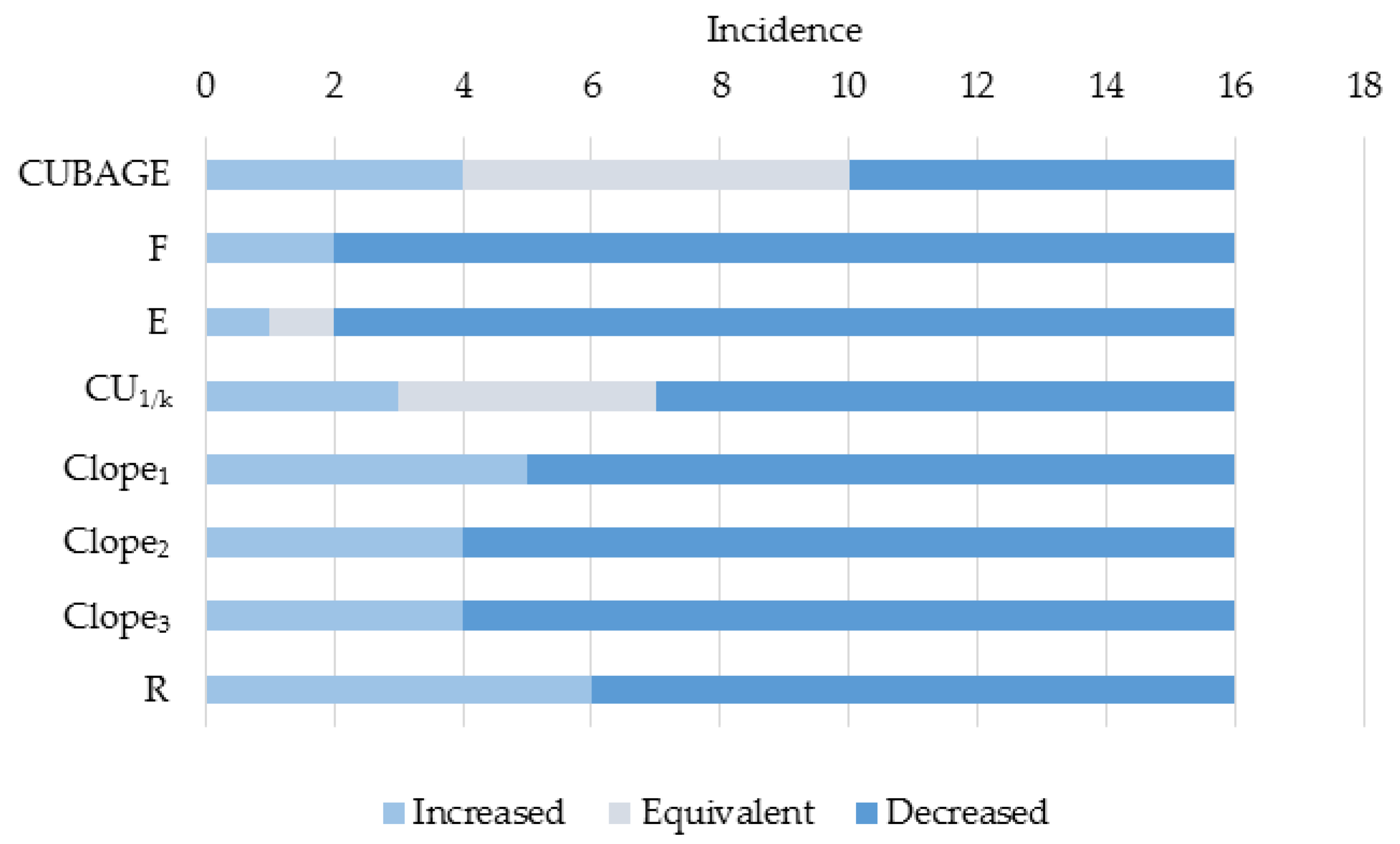
The NMI and ARI scores of the partitions chosen by each internal CVI in the k-modes clustering are shown in

Table 8. Average NMI values of the chosen k-modes partitions over 100 runs (k ranging from 2–10).

Dataset	CUBAGE	−F	−E	CU1/k	Clope1	Clope2	Clope3	R
Voting	(1) 0.443	(8) 0.312	(7) 0.324	(1) 0.443	(3) 0.418	(3) 0.418	(3) 0.418	(6) 0.397
Breast	(1) 0.674	(6) 0.363	(7) 0.358	(1) 0.674	(8) 0.016	(4) 0.48	(5) 0.407	(3) 0.491
Mushroom	(1) 0.458	(5) 0.368	(4) 0.391	(3) 0.394	(8) 0.196	(2) 0.434	(6) 0.365	(7) 0.291
Soybean	(1) 0.838	(4) 0.746	(3) 0.752	(1) 0.838	(8) 0.492	(6) 0.553	(6) 0.553	(5) 0.572
Car	(5) 0.05	(2) 0.065	(1) 0.072	(3) 0.058	(6) 0.026	(6) 0.026	(6) 0.026	(4) 0.054
Heart	(1) 0.206	(3) 0.175	(4) 0.171	(2) 0.205	(8) 0.039	(7) 0.165	(6) 0.165	(5) 0.167
Dermatology	(1) 0.704	(4) 0.647	(3) 0.684	(1) 0.704	(8) 0.313	(6) 0.362	(5) 0.456	(7) 0.321
Zoo	(2) 0.808	(3) 0.795	(4) 0.783	(5) 0.579	(8) 0.479	(7) 0.481	(1) 0.823	(6) 0.572
Average NMI *	0.522	0.434	0.442	0.487	0.247	0.365	0.402	0.358
Average Rank *	1.625	4.375	4.125	2.125	7.125	5.125	4.75	5.375

* Averaged over datasets (average values of each column).

,

Table 9. Average ARI values of the chosen k-modes partitions over 100 runs (k ranging from 2–10).

Dataset	CUBAGE	−F	−E	CU1/k	Clope1	Clope2	Clope3	R
Voting	(1) 0.53	(8) 0.174	(7) 0.191	(1) 0.53	(3) 0.503	(3) 0.503	(3) 0.503	(6) 0.428
Breast	(1) 0.787	(6) 0.217	(7) 0.195	(1) 0.787	(8) −0.001	(4) 0.551	(5) 0.337	(3) 0.639
Mushroom	(1) 0.489	(7) 0.187	(6) 0.228	(3) 0.319	(8) 0.155	(2) 0.447	(5) 0.268	(4) 0.309
Soybean	(1) 0.654	(4) 0.442	(3) 0.461	(1) 0.654	(8) 0.26	(6) 0.297	(6) 0.297	(5) 0.352
Car	(2) 0.023	(4) 0.017	(3) 0.021	(1) 0.025	(6) −0.001	(6) −0.001	(6) −0.001	(5) 0.014
Heart	(2) 0.199	(4) 0.092	(5) 0.079	(3) 0.19	(6) 0.065	(8) 0.055	(7) 0.065	(1) 0.263
Dermatology	(1) 0.552	(3) 0.493	(4) 0.487	(1) 0.552	(7) 0.136	(6) 0.159	(5) 0.21	(8) 0.119
Zoo	(1) 0.817	(3) 0.573	(4) 0.544	(5) 0.448	(7) 0.342	(8) 0.341	(2) 0.769	(6) 0.411
Average ARI *	0.506	0.274	0.276	0.438	0.183	0.294	0.306	0.317
Average Rank *	1.25	4.875	4.875	2	6.625	5.375	4.875	4.75

* Averaged over datasets (average values of each column).

,

Table 10. Average NMI values of the chosen k-modes partitions over 100 runs (k fixed to the actual number of classes).

Dataset	CUBAGE	−F	−E	CU1/k	Clope1	Clope2	Clope3	R
Voting	(1) 0.443	(5) 0.436	(1) 0.443	(1) 0.443	(6) 0.376	(6) 0.376	(6) 0.376	(4) 0.439
Breast	(1) 0.674	(4) 0.635	(1) 0.674	(1) 0.674	(8) 0.015	(7) 0.022	(6) 0.434	(5) 0.445
Mushroom	(1) 0.458	(5) 0.451	(1) 0.458	(1) 0.458	(8) 0.037	(1) 0.458	(6) 0.435	(7) 0.136
Soybean	(1) 1	(4) 0.977	(1) 1	(1) 1	(7) 0.675	(6) 0.692	(5) 0.791	(8) 0.672
Car	(4) 0.048	(1) 0.057	(3) 0.05	(2) 0.055	(7) 0.038	(8) 0.037	(6) 0.042	(5) 0.048
Heart	(2) 0.181	(3) 0.18	(7) 0.171	(5) 0.175	(4) 0.177	(8) 0.167	(6) 0.173	(1) 0.187
Dermatology	(3) 0.742	(4) 0.633	(1) 0.744	(2) 0.742	(7) 0.505	(6) 0.548	(5) 0.582	(8) 0.495
Zoo	(1) 0.852	(4) 0.818	(3) 0.836	(2) 0.838	(5) 0.811	(7) 0.804	(6) 0.809	(8) 0.781
Average NMI *	0.55	0.523	0.547	0.548	0.329	0.388	0.455	0.4
Average Rank *	1.75	3.75	2.25	1.875	6.5	6.125	5.75	5.75

* Averaged over datasets (average values of each column).

and

Table 11. Average ARI values of the chosen k-modes partitions over 100 runs (k fixed to the actual number of classes).

Dataset	CUBAGE	−F	−E	CU1/k	Clope1	Clope2	Clope3	R
Voting	(1) 0.53	(5) 0.511	(1) 0.53	(1) 0.53	(6) 0.451	(6) 0.451	(6) 0.451	(4) 0.53
Breast	(1) 0.787	(4) 0.738	(1) 0.787	(1) 0.787	(7) 0.008	(8) 0.001	(6) 0.488	(5) 0.513
Mushroom	(1) 0.489	(5) 0.486	(1) 0.489	(1) 0.489	(8) −0.015	(1) 0.489	(6) 0.465	(7) 0.023
Soybean	(1) 1	(4) 0.97	(1) 1	(1) 1	(7) 0.474	(6) 0.489	(5) 0.598	(8) 0.469
Car	(1) 0.036	(4) 0.03	(2) 0.034	(3) 0.032	(8) 0.006	(7) 0.009	(5) 0.022	(6) 0.012
Heart	(3) 0.134	(7) 0.107	(5) 0.123	(6) 0.119	(2) 0.22	(4) 0.124	(8) 0.104	(1) 0.277
Dermatology	(1) 0.654	(4) 0.52	(2) 0.63	(3) 0.621	(7) 0.26	(6) 0.298	(5) 0.343	(8) 0.236
Zoo	(3) 0.774	(8) 0.662	(6) 0.713	(7) 0.709	(2) 0.797	(5) 0.751	(4) 0.757	(1) 0.807
Average ARI *	0.551	0.503	0.538	0.536	0.275	0.326	0.403	0.358
Average Rank *	1.5	5.125	2.375	2.875	5.875	5.375	5.625	5

* Averaged over datasets (average values of each column).

.

When k was not determined (Table 8 and Table 9), CUBAGE outperformed the other indexes on most of the datasets, and CU_1/k came second. When k was determined (Table 10 and Table 11), CUBAGE still outperformed others, and indexes −E and −F advanced in performance.

5.4. Discussion

We can see from the overall results that none of the internal CVIs consistently outperformed all of the other CVIs in either of the benchmark evaluation criteria over the eight datasets. This is because that the datasets are of different structures, and that the benchmark criteria NMI and ARI do not always agree with each other, especially when the quality of the partition is relatively low (see Figure 6c,e,f). However, we can observe that index CUBAGE had better overall performance compared to others, from the perspectives of both the average scores and the averaged ranks. A detailed discussion follows:

Index E—the internal CVI without separation measure or assumption—performed well in the k-modes clustering when k was set to the actual number of classes. In the hierarchical clustering experiments, as we proved above, the value of E showed monotonicity with respect to the number of clusters, and the performance decreased notably. A similar performance drop appeared in the k-modes clustering when k was unknown.

Indexes F and R had lower sensitivities to the value distribution, since they only consider the most and/or the least common values in the cluster. The performances of these CVIs were below average in the experiments. The performance drop of F appeared when the number of clusters was unknown, similar to index E. As the compactness measure of F and R are equivalent, by comparing the trends in the hierarchical clustering experiments (Figure 6), we can observe that the compactness measure of R had little effect on the partition evaluation, and the role of the separation was dominant.

Index CU_1/k uses 1/k as the separation coefficient without respect to the value distribution between clusters. In the k-modes clustering experiments, the performance of CU_1/k dropped on most of the occasions when the number of clusters changed from known to unknown, as shown in Figure 7. This indicates that the separation assumption is not universally suitable, although it corrected the monotonicity of the compactness core.

The performance of the index Clope_r is highly dependent on the parameter r. As we discussed, the effect of compactness drops as r decreases. In the hierarchical clustering experiments, the value of Clope₁(P) monotonically decreased as the number of clusters increased under the effect of the separation measure. For the same reason, in the k-modes clustering, Clope₁(P) was outperformed by Clope₂(P) and Clope₃(P). However, Clope₂(P) and Clope₃(P) outperformed each other on different datasets, which indicates that setting r appropriately to compromise the compactness and the separation is difficult. Additionally, the performance drop of Clope_r when the number of clusters changed from known to unknown, as shown in Figure 7, indicates that the separation assumption of index Clope_r is not suitable for most datasets as well.

Such a performance drop happened least with our internal CVI—CUBAGE. The separation measure AGE showed advantageous applicability to the datasets and clustering methods, and coordinated well with the compactness measure E⁻¹. When the number of clusters was unknown, CUBAGE had improved performance compared to index E for introducing inter-cluster information. When the number was pre-known, the partitions chosen by E were identical to those chosen by CUBAGE on the datasets Voting, Breast, and Mushroom (datasets with two classes), which agreed with Equation (47); CUBAGE performed better than E on other datasets when k is fixed as well, which indicates that the separation measure AGE not only contributes to the performance of evaluating partitions of different sizes, it also has a positive impact when evaluating the partitions of the same size. For comparison, R was outperformed by its equivalent compactness measure F when k was fixed, and the separation coefficient of CU_1/k had no impact on the performance, since 1/k is a constant under such circumstances. As a result, CUBAGE performed better than other internal CVIs in general in the conducted experiments.

6. Conclusions and Future Work

This paper studies internal clustering validation measures for categorical data. We analyzed the compactness and separation measures or assumptions of five well-known internal CVIs, and proposed a new index—CUBAGE.

Analysis results showed that the indexes without separation measures based on the attribute distribution do not necessarily ignore the impact of separation, since some indexes (i.e., CU_1/k and Clope_r) adjusted the evaluation results by the separation assumptions with respect to the partition size or the object distribution, although the assumptions may be crude and not universally suitable.

The compactness cores of the indexes are all monotonic with respect to the number of clusters in the hierarchical clustering, which makes them biased toward partitions with more clusters. The separation measures or assumptions corrected such biases by their preferences for the concentrated partitions. Therefore, the coordination of separation and compactness affects the evaluation considerably. For instance, as discussed, the role of parameter r is to adjust the importance of the compactness and the separation of the index Clope_r, which influenced the effectiveness.

The proposed internal CVI—CUBAGE—is based on a new separation measure that uses the averaged information gain of isolating each cluster to measure the overall separation of the partition. Theoretical analysis showed that this separation measure scores the minimum possible value when the objects are least separated. Meanwhile, CUBAGE uses the reciprocal entropy of the dataset conditioned on the partition—which is also the reciprocal of index E—to measure the whole compactness. As the product of the separation and compactness measures, CUBAGE showed better performance in the experiments than other indexes, which indicates that the separation and the compactness measures are accurate, and that they coordinate well on most datasets.

In the future, we will investigate the internal CVIs in an extended range to provide systematic studies on the relation of within-cluster compactness and intracluster-separation. Secondly, the performance on evaluating the partitions of different characteristic patterns can be studied. Additionally, we will analyze the possibility of using CUBAGE as the objective function in the clustering process from the aspects, such as convergence speed.

References

1. Xu, R.; Ii, D.C.W. Survey of clustering algorithms. IEEE Trans. Neural Netw. 2005, 16, 645–678. [Google Scholar] [CrossRef] [PubMed]
2. Jain, A.K.; Dubes, R.C. Algorithms for clustering data. Technometrics 1988, 32, 227–229. [Google Scholar]
3. Cornuéjols, A.; Wemmert, C.; Gançarski, P.; Bennani, Y. Collaborative Clustering: Why, When, What and How. Inf. Fusion 2017, 39. [Google Scholar] [CrossRef]
4. Handl, J.; Knowles, J.; Kell, D.B. Computational cluster validation in post-genomic data analysis. Bioinformatics 2005, 21, 3201–3212. [Google Scholar] [CrossRef] [PubMed] [Green Version]
5. Halkidi, M.; Batistakis, Y.; Vazirgiannis, M. On Clustering Validation Techniques. J. Intell. Inf. Syst. 2001, 17, 107–145. [Google Scholar] [CrossRef]
6. Rand, W.M. Objective Criteria for the Evaluation of Clustering Methods. Publ. Am. Stat. Assoc. 1971, 66, 846–850. [Google Scholar] [CrossRef] [Green Version]
7. Vinh, N.X.; Epps, J.; Bailey, J. Information theoretic measures for clusterings comparison: Is a correction for chance necessary? In Proceedings of the International Conference on Machine Learning, Montreal, QC, Canada, 14–18 June 2009; pp. 1073–1080. [Google Scholar]
8. Rijsbergen, C.J.V. Information Retrieval; Butterworth-Heinemann: Oxford, UK, 1979; p. 777. [Google Scholar]
9. Bai, L.; Liang, J. Cluster validity functions for categorical data: A solution-space perspective. Data Min. Knowl. Discov. 2015, 29, 1560–1597. [Google Scholar] [CrossRef]
10. Li, H.; Zhang, S.; Ding, X.; Zhang, C.; Dale, P. Performance evaluation of cluster validity indices (CVIs) on Multi/Hyperspectral remote sensing datasets. Remote Sens. 2016, 8, 295. [Google Scholar] [CrossRef] [Green Version]
11. Harimurti, R.; Yamasari, Y.; Ekohariadi; Munoto; Asto, B.I.G.P. Predicting student’s psychomotor domain on the vocational senior high school using linear regression. In Proceedings of the 2018 International Conference on Information and Communications Technology (ICOIACT), Yogyakarta, Indonesia, 6–8 March 2018; pp. 448–453. [Google Scholar]
12. Luna-Romera, J.M.; García-Gutiérrez, J.; Martínez-Ballesteros, M.; Santos, J.C.R. An approach to validity indices for clustering techniques in Big Data. Prog. Artific. Intell. 2018, 7, 81–94. [Google Scholar] [CrossRef]
13. Rizzoli, P.; Loder, E.; Joshi, S. Validity of Cluster Diagnosis in an Electronic Health Record. Headache 2016, 56, 1132–1136. [Google Scholar] [CrossRef] [PubMed]
14. Aggarwal, C.C.; Procopiuc, C.; Yu, P.S. Finding localized associations in market basket data. IEEE Trans. Knowl. Data Eng. 2002, 14, 51–62. [Google Scholar] [CrossRef] [Green Version]
15. Barbará, D.; Jajodia, S. Applications of Data Mining in Computer Security; Kluwer Academic Publishers: Boston, MA, USA, 2002. [Google Scholar]
16. Yang, Y. An Evaluation of Statistical Approaches to Text Categorization. Inf. Retr. 1999, 1, 69–90. [Google Scholar] [CrossRef]
17. Liu, Y.; Li, Z.; Xiong, H.; Gao, X.; Wu, J.; Wu, S. Understanding and enhancement of internal clustering validation measures. IEEE Trans. Cybern. 2013, 43, 982–994. [Google Scholar] [PubMed]
18. Kremer, H.; Kranen, P.; Jansen, T.; Seidl, T.; Bifet, A.; Holmes, G.; Pfahringer, B. An effective evaluation measure for clustering on evolving data streams. In Proceedings of the ACM SIGKDD International Conference on Knowledge Discovery and Data Mining, San Diego, CA, USA, 21–24 August 2011; pp. 868–876. [Google Scholar]
19. Song, M.; Zhang, L. Comparison of Cluster Representations from Partial Second- to Full Fourth-Order Cross Moments for Data Stream Clustering. In Proceedings of the Eighth IEEE International Conference on Data Mining, Pisa, Italy, 15–19 December 2009; pp. 560–569. [Google Scholar]
20. Xiong, H.; Wu, J.; Chen, J. K-means clustering versus validation measures: A data distribution perspective. IEEE Trans. Syst. Man Cybern. Part B Cybern. 2009, 39, 318–331. [Google Scholar] [CrossRef] [PubMed]
21. Brun, M.; Chao, S.; Hua, J.; Lowey, J.; Carroll, B.; Suh, E.; Dougherty, E.R. Model-based evaluation of clustering validation measures. Pattern Recognit. 2007, 40, 807–824. [Google Scholar] [CrossRef] [Green Version]
22. Tan, P.N.; Steinbach, M.; Kumar, V. Introduction to Data Mining, 1st ed.; Addison-Wesley Longman Publishing Co., Inc.: Boston, MA, USA, 2005; pp. 86–103. [Google Scholar]
23. Halkidi, M.; Batistakis, Y.; Vazirgiannis, M. Cluster validity methods: Part I. ACM SIGMOD Rec. 2002, 31, 40–45. [Google Scholar] [CrossRef]
24. Zhang, G.X.; Pan, L.Q. A Survey of Membrane Computing as a New Branch of Natural Computing. Chin. J. Comput. 2010, 33, 208–214. [Google Scholar] [CrossRef]
25. Busi, N. Using well-structured transition systems to decide divergence for catalytic P systems. Theor. Comput. Sci. 2007, 372, 125–135. [Google Scholar] [CrossRef]
26. An Approximate Algorithm for NP-Complete Optimization Problems Exploiting P-systems. Available online: http://bioinfo.uib.es/~recerca/BUM/nishida.pdf (accessed on 10 November 2004).
27. Maulik, U.; Bandyopadhyay, S. Performance Evaluation of Some Clustering Algorithms and Validity Indices; IEEE Computer Society: Washington, WA, USA, 2002; pp. 1650–1654. [Google Scholar]
28. Pal, N.R.; Bezdek, J.C. On cluster validity for the fuzzy c-means model. IEEE Trans. Fuzzy Syst. 2002, 3, 370–379. [Google Scholar] [CrossRef]
29. Lei, Y.; Bezdek, J.C.; Romano, S.; Vinh, N.X.; Chan, J.; Bailey, J. Ground truth bias in external cluster validity indices. Pattern Recognit. 2017, 65, 58–70. [Google Scholar] [CrossRef] [Green Version]
30. Barbará, D.; Li, Y.; Couto, J. COOLCAT: An entropy-based algorithm for categorical clustering. In Proceedings of the Eleventh International Conference on Information and Knowledge Management, McLean, VA, USA, 4–9 November 2002; pp. 582–589. [Google Scholar]
31. Huang, Z. A Fast Clustering Algorithm to Cluster Very Large Categorical Data Sets in Data Mining. Res. Issues Data Min. Knowl. Discov. 1997, 1–8. [Google Scholar]
32. Gluck, M. Information, Uncertainty and the Utility of Categories. In Proceedings of the Seventh Annual Conference on Cognitive Science Society, Irvine, CA, USA, 15–17 August 1985; pp. 283–287. [Google Scholar]
33. Yang, Y.; Guan, X.; You, J. CLOPE:a fast and effective clustering algorithm for transactional data. In Proceedings of the Eighth ACM SIGKDD International Conference on Knowledge Discovery and Data Mining, Edmonton, AB, Canada, 23–25 July 2002; pp. 682–687. [Google Scholar]
34. Chang, C.H.; Ding, Z.K. Categorical Data Visualization and Clustering Using Subjective Factors. Data Knowl. Eng. 2005, 53, 243–262. [Google Scholar] [CrossRef]
35. Shannon, C.E. A mathematical theory of communication. Bell Labs Tech. J. 1948, 27, 379–423. [Google Scholar] [CrossRef]
36. Macqueen, J. Some Methods for Classification and Analysis of MultiVariate Observations. In Proceedings of the Berkeley Symposium on Mathematical Statistics and Probability, Berkeley, CA, USA, 21 June–18 July 1965; pp. 281–297. [Google Scholar]
37. Fisher, D.H. Knowledge acquisition via incremental conceptual clustering. Mach. Learn. 1987, 2, 139–172. [Google Scholar] [CrossRef] [Green Version]
38. Witten, I.; Frank, E.; Hall, M.; Hall, M. Data Mining: Practical Machine Learning Tools and Techniques, Third Edition (The Morgan Kaufmann Series in Data Management Systems). ACM SIGMOD Rec. 2011, 31, 76–77. [Google Scholar] [CrossRef]
39. Li, Y.; Le, J.; Wang, M. Improving CLOPE’s profit value and stability with an optimized agglomerative approach. Algorithms 2015, 8, 380–394. [Google Scholar] [CrossRef]
40. Campo, D.N.; Stegmayer, G.; Milone, D.H. A new index for clustering validation with overlapped clusters. Expert Syst. Appl. 2016, 64, 549–556. [Google Scholar] [CrossRef]
41. Dziopa, T. Clustering Validity Indices Evaluation with Regard to Semantic Homogeneity. In Proceedings of the 2016 Federated Conference on Computer Science and Information Systems, Gdansk, Poland, 11–14 September 2016; pp. 3–9. [Google Scholar]
42. Oszust, M.; Kostka, M. Evaluation of Subspace Clustering Using Internal Validity Measures. Adv. Electr. Comput. Eng. 2015, 15, 141–146. [Google Scholar] [CrossRef]
43. Desgraupes, B. Clustering Indices; University of Paris Ouest-Lab Modal’X: Nanterre, France, 2013; p. 34. [Google Scholar]
44. Baarsch, J.; Celebi, M.E. Investigation of internal validity measures for K-means clustering. In Proceedings of the International Multiconference of Engineers and Computer Scientists, HongKong, China, 14–16 March 2012; pp. 14–16. [Google Scholar]
45. Zhao, Q. Cluster Validity in Clustering Methods; University of Eastern Finland: Kuopio, Finland, 2012. [Google Scholar]
46. Rendon, E.; Abundez, I.; Arizmendi, A.; Quiroz, E.M. Internal versus external cluster validation indexes. Int. J. Comput. Commun. 2011, 5, 27–34. [Google Scholar]
47. Ingaramo, D.; Pinto, D.; Rosso, P.; Errecalde, M. Evaluation of internal validity measures in short-text corpora. In Proceedings of the International Conference on Intelligent Text Processing and Computational Linguistics, Haifa, Israel, 17–23 February 2008; pp. 555–567. [Google Scholar]
48. Halkidi, M.; Vazirgiannis, M. Clustering validity assessment: Finding the optimal partitioning of a data set. In Proceedings of the 2001 IEEE International Conference on Data Mining, San Jose, CA, USA, 29 November–2 December 2001; pp. 187–194. [Google Scholar]
49. Jiang, D.; Tang, C.; Zhang, A. Cluster analysis for gene expression data: A survey. IEEE Trans. Knowl. Data Eng. 2004, 16, 1370–1386. [Google Scholar] [CrossRef]
50. Wu, J.; Chen, J.; Xiong, H.; Xie, M. External validation measures for K-means clustering: A data distribution perspective. Expert Syst. Appl. 2009, 36, 6050–6061. [Google Scholar] [CrossRef]
51. Jensen, J.L.W.V. Sur les fonctions convexes et les inégalités entre les valeurs moyennes. Acta Math. 1906, 30, 175–193. [Google Scholar] [CrossRef]
52. Cover, T.M.; Thomas, J.A. Elements of Information Theory; Wiley: New York, NY, USA, 1991; pp. 155–183. [Google Scholar]
53. Quinlan, J.R. Induction of Decision Trees. Mach. Learn. 1986, 1, 81–106. [Google Scholar] [CrossRef]
Figure 1. Clustering procedure consists of four steps with a feedback pathway.
Algorithms 11 00177 g001
Figure 2. This figure illustrates how the information gain of separating each clusters GEl are calculated and averaged to represent the whole separation of the partition. In the figure, HU is the entropy of unpartitioned dataset U (n objects), Hl is the entropy of cluster l (nl objects), and Hrest is the entropy of the rest of the objects.
Algorithms 11 00177 g002
Figure 3. Flowchart of CUBAGE.
Algorithms 11 00177 g003
Figure 4. Procedures of the hierarchical and k-modes clustering validation experiments.
Algorithms 11 00177 g004
Figure 5. Determining the external index value of the partition selected by an internal index, where IV and EV are the values of the internal and the external index, respectively.
Algorithms 11 00177 g005
Figure 6. The validation scores of each layer of the hierarchy on different datasets. On axis OX are the layers, i.e., partitions of different size; on axis OY are the values of the validation (quality) of each partition measured by different CVIs. Note that the values of Cloper(P) with the parameter r = 1~3 have been normalized for convenience of comparison.
Algorithms 11 00177 g006aAlgorithms 11 00177 g006b
Figure 7. The number of incidences of increased, equivalent, and decreased performances in both NMI and ARI when the number of clusters changes from pre-known to unknown in the k-modes clustering.
Algorithms 11 00177 g007