Inapproximability of Rank, Clique, Boolean, and Maximum Induced Matching-Widths under Small Set Expansion Hypothesis

Abstract

Wu et al. (2014) showed that under the small set expansion hypothesis (SSEH) there is no polynomial time approximation algorithm with any constant approximation factor for several graph width parameters, including tree-width, path-width, and cut-width (Wu et al. 2014). In this paper, we extend this line of research by exploring other graph width parameters: We obtain similar approximation hardness results under the SSEH for rank-width and maximum induced matching-width, while at the same time we show the approximation hardness of carving-width, clique-width, NLC-width, and boolean-width. We also give a simpler proof of the approximation hardness of tree-width, path-width, and cut-widththan that of Wu et al.

1. Introduction

There are many graph width parameters, such as cut, path, tree, band, branch, carving, clique, NLC, rank, boolean, maximum induced matching-widths, and the approximability and inapproximability of some of these width parameters have been investigated extensively. For example, regarding the approximability of tree-width $tw$, it is known that there are polynomial time approximation algorithms with ratio $O(\sqrt{logtw(G)})$ [1]. Regarding inapproximability, tree-width cannot be approximated within any additive constant c unless P = NP [2]. Regarding rank-width $rw$, for every fixed k, there is a polynomial time algorithm that reports $rw(G)>k$, or outputs a rank decomposition of width at most $3k-1$ [3]. Recently, it has been shown that maximum induced matching-width cannot be approximated within any constant factor in polynomial time unless NP = ZPP [4]. For several graph parameters, there are still large gaps between approximability and inapproximability results: it is a major concern as to whether there are constant factor approximation algorithms for those graph width parameters. Indeed, it is a long-standing open problem as to whether tree-width can be approximated within a constant factor.

Raghavendra and Steurer introduced a complexity assumption referred to as the small set expansion hypothesis (SSEH) that is deeply related to the unique games conjecture (UGC) [5], and since then several inapproximability results under SSEH have been reported. For example, in [6] Raghavendra et al. showed that under SSEH there are no constant factor approximation algorithms for the balanced separator and minimum linear arrangement problems (a similar result was already known for the balanced separator problem under UGC [7]). Recently, Manurangsi showed inapproximability results for maximum biclique problems, minimum k-cut, and densest at-least-k-subgraph [8]. In [9], Wu et al. (2014) showed under SSEH that there are no constant factor approximation algorithms for cut, path, tree-widths, minimum fill-in (it has recently been shown that minimum fill-in has no polynomial time approximation scheme unless P = NP and that assuming ETH, there is some positive $\epsilon$ such that no algorithm can find a (1 + $\epsilon$) approximation in time $2^{O(n^{1-\delta })}$ for any positive constant $\delta$ [10]), one-shot black pebbling costs, and other problems. Those were the first results showing the hardness of constant factor approximation for these graph parameters. However, the hardness result of tree-width in [9] does not necessarily mean that the long-standing open problem of tree-width is solved, because there is no consensus on the correctness of UGC and SSEH at this time [11] and it was shown in [12] that both unique games and small set expansion admit a subexponential time approximation algorithm. Regardless of the veracity of these two assumptions, the results in [6,9] stimulate the study of approximation hardness for graph parameters, and it is widely acknowledged that UGC and SSEH have played important roles in the study of approximation algorithms.

The above width parameters have widespread applications from both theoretical and practical viewpoints (e.g., [13]). Efficiently computing these width parameters becomes especially relevant when considering the fact that many NP-hard problems admit efficient graph algorithms for instances whose width parameters have a small value. The reader is invited to refer to the literature on fixed parameter tractability for further information (e.g., Downey and Fellow [14], Cygan et al. [15], Flum and Grohe [16]). Inspired by [9], in this paper, we extend the research in [9] to other graph parameters. That is, we demonstrate in a unified manner that under SSEH there are no constant factor polynomial time approximation algorithms for cut, path, tree, branch, carving, NLC, rank, clique, boolean, and maximum induced matching-widths (see Figure 1 in Section 4).

2. Definitions and Known Results

2.1. Graphs, Expansion, Matrices

In this subsection, we recall some definitions and notation of graphs, expansion, and matrices. Let G be a simple graph. We use operators V and E to refer to the vertex and edge sets of G as $V(G)$ and $E(G)$, respectively. We will frequently write $G=(V,E)$ instead of $G=(V(G),E(G))$. For a subset X of $V(G)$ ($E(G)$, resp.), $\overline{X}$ denotes $V(G)\backslash X$ ($E(G)\backslash X$, resp.). Let X and Y be subsets of V. $N(X)$ denotes the neighbors of X (i.e., $N(X)=\{u\in \overline{X}\mid \exists v\in X$ s.t. $\{u,v\}\in E\}$). $E(X,Y)$ denotes $\left\{\right\{u,v\}\in E:u\in X,v\in Y\}$. For each $v\in V$, $d_G(v)$ (or simply $d(v)$) denotes the degree of v in G. $\Delta (G)$ denotes the maximum degree of G. $G\left[X\right]$ denotes the induced subgraph of G induced by X. The vertex boundary width of order i of G, denoted by $b_v(i,G)$, is defined as $b_v(i,G):={min}_{S\subseteq V,\left|S\right|=i}\left|N(S)\right|$. Similarly, the edge boundary width of order i, denoted by $b_e(i,G)$, is defined as $b_e(i,G):={min}_{S\subseteq V,\left|S\right|=i}\left|E(S,\overline{S})\right|$.

Let S be a subset of V. The edge expansion $\Phi (S)$ is defined as ${\Phi }_G(S)=\frac{|E(S,\overline{S})|}{min\{\mathsf{vol}(S),\mathsf{vol}(\overline{S})\}}$, where $\mathsf{vol}(S)={\sum }_{v\in S}d(v)$. Moreover, $\mu (S)$ denotes $\frac{\mathsf{vol}(S)}{\mathsf{vol}(V)}$. Since, in this paper, we mainly consider d-regular graphs, $\mathsf{vol}(S)$ and $\mu (S)$ can be regarded as $d\left|S\right|$ and $\frac{\left|S\right|}{\left|V\right|}$, respectively.

Let M be the adjacency matrix of G. For $X,Y\subseteq V$ such that $X\cap Y=\varnothing$, $M[X,Y]$ means a matrix satisfying the following. The rows and columns are labeled by X and Y, respectively, and each entry $(x,y)$ with $x\in X$ and $y\in Y$ is 1 if $\{x,y\}\in E(G)$, 0 otherwise. We denote the rank over $GF(2)$ of $M[X,Y]$ as $\mathit{rank}(M[X,Y])$. For the rank over $GF(2)$, the following is known.

Lemma 1

(Lemma 4.3 in [17]). Let A be a matrix over $GF(2)$ such that A has at least p non-zero entries and each row and each column in A has at most q non-zero entries. Then, $\mathit{rank}(A)\ge \frac{p}{q^2}$ holds.

2.2. Graph Width Parameters

In this subsection, we briefly review the definitions of graph width parameters. We only give the definitions of graph width parameters that will be needed in our proofs. Definitions of the other graph width parameters can be found as follows: For the definitions of path-width, tree-width, branch-width, and band-width, see e.g., [18]. For the definitions of carving-width, clique-width, and boolean-width, see e.g., [19,20,21], respectively. Note that the decision problems related to graph width parameters considered in this paper are all minimization problems.

As some of graph width parameters are based on decomposition trees, let us first review the notion of a decomposition tree. Given a tree T, let us denote the set of leaves of T by $L(T)$. For an edge e in T, ${(T\backslash e)}_1$ and ${(T\backslash e)}_2$ denote the two subtrees obtained from T by removing e. Given a graph $G=(V,E)$ and a tree T such that $|L(T)|=\left|V\right|$, let $f_T$ be a bijection from $L(T)$ to V. For each edge e in T, we denote the subset of V mapped by $f_T$ from the leaves in ${(T\backslash e)}_i$ as ${(V\backslash e)}_i$ for $i\in \{1,2\}$. That is, ${(V\backslash e)}_i=\{f_T(v):v\in L({(T\backslash e)}_i)\}$. Note that ${(V\backslash e)}_i$ obviously depends on T and $f_T$. In this paper, we will refer to a pair $(T,f_T)$ satisfying the following conditions as a decomposition tree of $G=(V,E)$:

• T is a subcubic tree with $\left|V\right|$ leaves, where a tree is subcubic if every vertex in T has degree 1 or 3;
• $f_T$ is a bijection from $L(T)$ of T to V.

We denote the set of tree decompositions of G by ${\mathcal{D}}_G$.

Cut-width: 

For a graph $G=(V,E)$, let $\pi :V\to \{1,\dots ,|V\left|\right\}$ be an ordering of V. Let $S_{\pi }(i):=$$\{{\pi }^{-1}(1),$${\pi }^{-1}(2),$$\dots ,$${\pi }^{-1}(i)\}$, ${\partial }_e(\pi ,i):=E(S_{\pi }(i),\overline{S_{\pi }(i)})$. Then, ${\displaystyle cutw(G):=\underset{\pi }{min}\underset{1\le i\le n}{max}\left|{\partial }_e(\pi ,i)\right|}$.

Rank-width: 

For a graph $G=(V,E)$, let T be a subcubic tree and $f_T$ be a bijection from $L(T)$ to V. Then, ${\displaystyle rw(G):=\underset{(T,f_T)\in {\mathcal{D}}_G}{min}\underset{e\in E(T)}{max}rank\left(M\left[{(V\backslash e)}_1,{(V\backslash e)}_2\right]\right)}$.

Maximum induced matching-width 

For a graph $G=(V,E)$ and a subset A of V, we denote the size of a maximum induced matching in the bipartite graph $(A,\overline{A};E(A,\overline{A}))$ by $mim(A)$. Then, ${\displaystyle mimw(G):=\underset{(T,f_T)\in {\mathcal{D}}_G}{min}\underset{e\in E(T)}{max}mim({(V\backslash e)}_1))}$.

3. SSE Hypothesis

In this section, we briefly review the small set expansion hypothesis (SSEH), which is deeply related to the unique games conjecture (UGC). Research on the unique games conjecture and semidefinite programming has led to significant progress in the field of approximation algorithms in the past decade. In [9], Wu et al. provided the following very useful strong form of SSEH.

SSE hypothesis (strong form) [Conjecture 2.23 and Remark 2.25 in [9]] There is a constant c such that for every integer $q>1$ and arbitrarily small $\epsilon >0$, the following problem is NP-hard:

Problem 1.

Given a regular graph $G=(V,E)$, distinguish between the following two cases:

Yes 

There exist q disjoint sets $S_1,\dots ,S_q\subseteq V$ such that ${\Phi }_G(S_i)\le 2\epsilon$ and $|S_i|=\frac{\left|V\right|}{q}$ holds for all $1\le i\le q$,

No 

For every $\frac{\left|V\right|}{10}\le \left|S\right|\le \frac{9\left|V\right|}{10}$, ${\Phi }_G(S)\ge c\sqrt{\epsilon }$ holds.

4. Method for Showing Inapproximability

In this section, we explain the useful method which is used implicitly in [9] to prove the inapproximability of width parameters in a unified setting. Through the remainder of this section, $gw$ denotes a graph width parameter such that determining $gw$ is a minimization problem and P denotes any polynomial time computable parameter of G, typically $\left|V\right|$ or $\left|E\right|$. That is, the graph parameters $gw$ and P are functions from graphs to the natural numbers such that isomorphic graphs are mapped to the same number.

To show the approximation hardness of $gw$, it is sufficient to prove that there are constants $c_Y$ and $c_N$ such that for any graph G,

• $gw(G)\le c_Y\epsilon P$ holds if G is a YES instance in Problem 1 (i.e., completeness), and
• $gw(G)\ge c_N\sqrt{\epsilon }P$ holds if G is a NO instance in Problem 1 (i.e., soundness),

where $\epsilon$ is the same as in Problem 1. We will refer to such $c_Y\epsilon P$ ($c_N\sqrt{\epsilon }P$, resp.) as upper threshold (lower threshold, resp.).

Suppose that $gw(G)$ can be approximated within a constant factor in polynomial time. That is, there is a constant $\rho >0$ for which there is an approximation algorithm A such that for any graph G, A outputs a value $A(G)$ satisfying $gw(G)\le A(G)\le \rho ·gw(G)$. Then, take $\epsilon$ such that $\frac{1}{\rho }>\frac{c_Y\sqrt{\epsilon }}{c_N}$. That is, $\epsilon <{\left(\frac{c_N}{c_Y}·\frac{1}{\rho }\right)}^2$. Then, the following Algorithm 1, which uses the approximation algorithm A as a subroutine, solves Problem 1.

Algorithm 1 DeciInstByAlg$A(G)$

Input: a graph G Output: YES/NO

The correctness of Algorithm 1 can be explained as follows. In the case of “$A(G)<c_N\sqrt{\epsilon }P$”, from $gw(G)\le A(G)<c_N\sqrt{\epsilon }P$, we can guarantee that G is not a NO instance by the soundness condition. In the case of “$A(G)\ge c_N\sqrt{\epsilon }P$”, from $gw(G)\ge \frac{A(G)}{\rho }\ge \frac{c_N\sqrt{\epsilon }}{\rho }P>c_N\sqrt{\epsilon }·\frac{c_Y\sqrt{\epsilon }}{c_N}P\ge c_Y\epsilon P$, we can conclude that G is not a YES instance by the completeness condition.

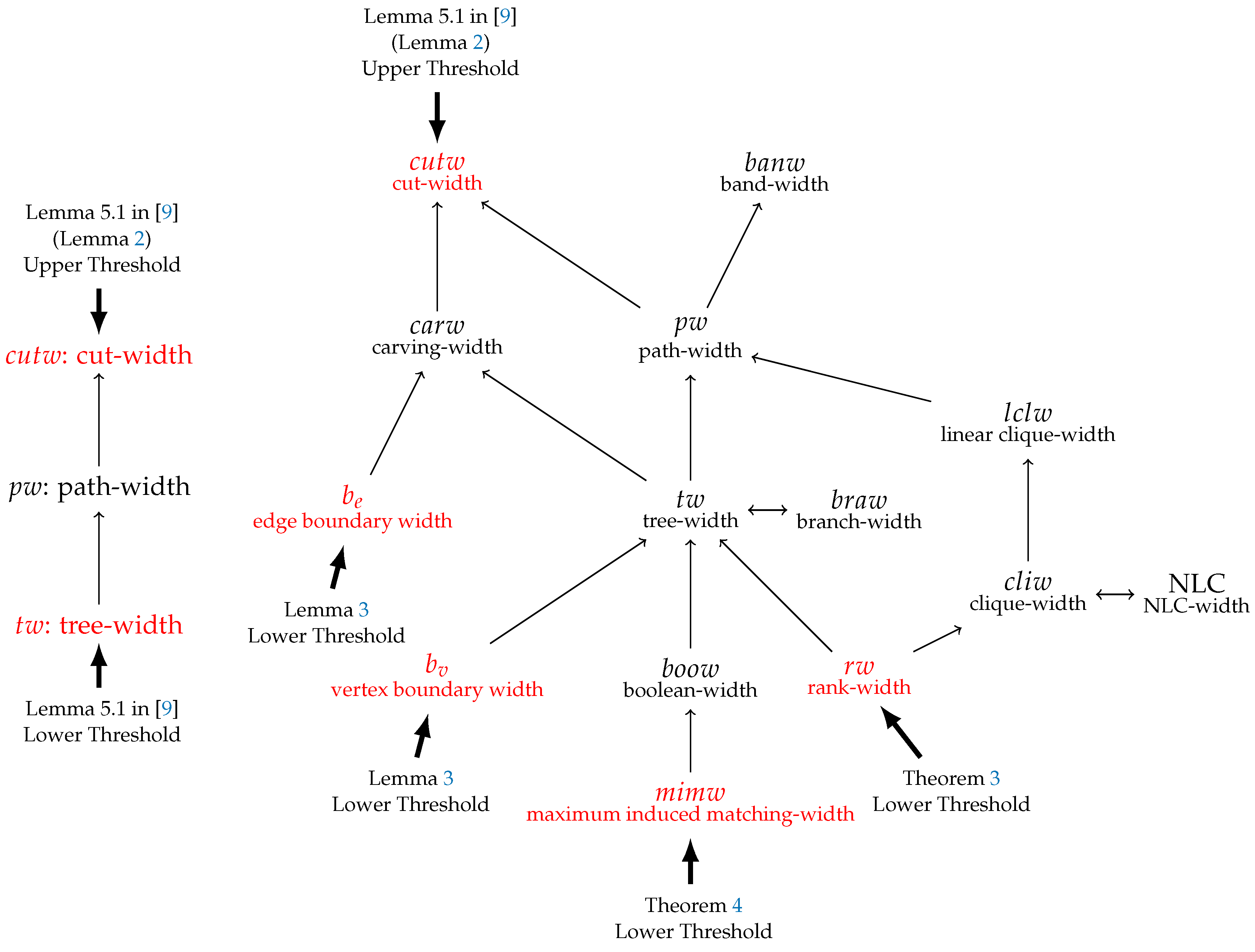
It is worth mentioning that for graph width parameters $g{w}_i$ ($1\le i\le 3$) such that $g{w}_1(G)⪯g{w}_2(G)⪯g{w}_3(G)$ for any graph G, the approximation hardness of $g{w}_i$ ($1\le i\le 3$) can be shown by just showing both the completeness for $g{w}_3$ and soundness for $g{w}_1$, where $g{w}_i(G)⪯g{w}_{i+1}(G)$ means that there exists a constant c such that $g{w}_i(G)\le c·g{w}_{i+1}(G)$ for any G. Figure 1 illustrates the unified setting: two width parameters $g{w}_u$ and $g{w}_l$ such that $g{w}_u$ is arranged above $g{w}_l$ are linked by a line if $g{w}_l⪯g{w}_u$ holds. In the figure, $lclw$ means linear clique-width, and the left (right, resp.) side illustrates a scheme of proofs for the inapproximability in [9] (this paper, resp.). The relations among width parameters illustrated in Figure 1 can be confirmed from the inequalities in Appendix A.

5. Hardness Results Derived from Inapproximability of Tree-Width

In this section, we exhibit approximation hardness results for several graph width parameters which can be derived from the approximation hardness of tree-width together with known results.

Theorem 1.

Assume that tree-width cannot be approximated within any constant factor in polynomial time. Then, {branch, carving, clique}-widths cannot be approximated within any constant factor either.

Proof. 

The approximation hardness of branch-width follows from the fact that $braw(G)-1\le tw(G)\le \lfloor \frac{3}{2}\times braw(G)\rfloor -1$ [18].

For carving-width, it is known that from a graph G we can construct a graph $G^{\prime }$ in polynomial time such that $tw(G)\le tw(G^{\prime })\le tw(G)+1$ and $\Delta (G^{\prime })\le 3$ [22]. It is also known that $\frac{carw(G)}{\Delta (G)}\le tw(G)\le 2\times carw(G)$ [23,24,25]. By combining both results, we can conclude that if carving-width can be approximated within a constant factor, then tree-width can be approximated within a constant factor as well.

The hardness of clique-width can be shown by the fact that $\frac{tw(G)+1}{4}\le cliw(L(G))\le 2tw(G)+2$ [26], where $L(G)$ means the line graph of G. □

6. Results

6.1. Simpler Proof of the Inapproximability of {Cut, Path, Tree}-Widths

As mentioned in Section 1, in [9], Wu et al. demonstrated that under SSEH there are no constant factor approximation algorithms for cut-width, path-width, and tree-width. In this subsection, we show the same result in a different way from that of Wu et al. The difference is as follows. Recall first the relations $cutw(G)\ge pw(G)\ge tw(G)$. To show the approximation, hardness, completeness, and soundness should be proved (see Section 4). To prove completeness, Wu et al. gave an upper threshold of cut-width, and we just use their upper threshold, so there is no difference in this part. To prove soundness, they gave a lower threshold of tree-width. To obtain the lower threshold, they used the lower bound of “1/2-vertex separator”, which is a well-known lower bound of tree-width. Instead of the 1/2-vertex separator, we employ the vertex boundary width, which is also known as a lower bound of tree-width. The most obvious difference is that they used an auxiliary graph $G^{\prime }$ produced from an input graph G to show a lower bound of 1/2-vertex separator of $G^{\prime }$, while in our case, we do not need an auxiliary graph. In this sense, our proof is simpler than that of Wu et al. (2014). To be self-contained, we review the proof of the completeness of Theorem 4.1 in [9].

Lemma 2

(Completeness of Theorem 4.1 in [9]). Let $q=\frac{1}{\epsilon }$. Let $G=(V,E)$ be d-regular and a YES instance in Problem 1, where d is an universal constant. Then, $cutw(G)\le c_c\epsilon \left|E\right|$ holds for some universal constant $c_c$.

Proof. 

Since G is a YES instance, we have

$$|E(S_i,V\backslash S_i)|={\Phi }_G(S_i)\times d\left|S_i\right|={\Phi }_G(S_i)\times d\frac{\left|V\right|}{q}={\Phi }_G(S_i)\times \frac{2\left|E\right|}{q}\le \frac{4\epsilon \left|E\right|}{q}.$$

Hence, the number of edges whose endpoints do not belong to the same partition $S_i$ is upper-bounded as follows:

$$\frac{1}{2}\sum _{i=1}^q|E(S_i,V\backslash S_i)|\le \frac{1}{2}\sum _{i=1}^q\frac{4\epsilon \left|E\right|}{q}\le 2\epsilon \left|E\right|.$$

From $\frac{1}{q}=\epsilon$, we have $|S_i|=\epsilon |V|$. Hence, $|E(S_i,S_i)|$ is at most $\frac{d|S_i|}{2}=\frac{d\epsilon \left|V\right|}{2}=\epsilon \left|E\right|$. Thus, by considering an ordering in which u comes before v for any vertices of $u\in S_i$ and $v\in S_j$ with $i<j$, we have $cutw(G)\le 3\epsilon \left|E\right|$ (i.e., $c_c=3$).

We now show the soundness in Lemma 3.

Lemma 3.

Let $G=(V,E)$ be a NO instance stated in Problem 1. Then, for all $\frac{\left|V\right|}{4}\le i\le \frac{\left|V\right|}{2}$,

• ${min}_i{b}_e(i,G)\ge \frac{c}{2}\sqrt{\epsilon }\left|E\right|$, and
• ${min}_i{b}_v(i,G)\ge \frac{c}{2d}\sqrt{ϵ}\left|E\right|$

hold, where c is the constant in the NO instance in Problem 1.

Proof. 

For each $\frac{\left|V\right|}{4}\le i\le \frac{\left|V\right|}{2}$, let $S^i$ be a set such that $b_e(i,G)=\left|E(S^i,\overline{S^i})\right|$ and $|S^i|=i$. Then, for each i, we have $b_e(i,G)=|E(S^i,\overline{S^i})|={\Phi }_G(S^i)\times d|S^i|\ge c\sqrt{ϵ}\times d\times i\ge c\sqrt{ϵ}\times d\times \frac{\left|V\right|}{4}=\frac{c}{2}\sqrt{ϵ}\times \left|E\right|$.

Let $S^i$ be a set such that $b_v(i,G)=\left|N(S^i)\right|$ and $|S^i|=i$. From the above and the fact that $|E(S,\overline{S})|\le |N(S)|\times d$, we have

$$\begin{array}{ccc}\hfill \underset{\frac{\left|V\right|}{4}\le i\le \frac{\left|V\right|}{2}}{min}{b}_v(i,G)& =& \underset{\frac{\left|V\right|}{4}\le i\le \frac{\left|V\right|}{2}}{min}\left|N(S^i)\right|\ge \underset{\frac{\left|V\right|}{4}\le i\le \frac{\left|V\right|}{2}}{min}\frac{|E(S^i,\overline{S^i})|}{d}\hfill \\ & \ge & \frac{1}{d}\times \underset{\frac{\left|V\right|}{4}\le i\le \frac{\left|V\right|}{2}}{min}|E(S^i,\overline{S^i})|\ge \frac{1}{d}\times \frac{c}{2}\sqrt{ϵ}\left|E\right|.\hfill \end{array}$$

Theorem 2.

Under SSEH, it is NP-hard to approximate $\{cutw,pw,tw,carw\}$-widths of a graph to within a constant factor in polynomial time.

Proof. 

Combining Lemmas 2 and 3 and the relations: for each $1\le j\le \left|V\right|$,

• ${min}_{j/2\le i\le j}{b}_v(i,G)-1\le tw(G)\le pw(G)\le min\{cutw(G),banw(G)\}$ [27],
• ${min}_{j/2\le i\le j}{b}_v(i,G)\le {min}_{j/2\le i\le j}{b}_e(i,G)\le carw(G)\le cutw(G)$ [28],

we have the theorem. □

6.2. Inapproximability of Rank, Clique, Boolean, and Mim-Widths

Theorem 3.

Under SSEH, it is NP-hard to approximate $rank$ and $clique$-widths of a graph to within a constant factor in polynomial time.

Proof. 

Let $G=(V,E)$ be a YES instance stated in Problem 1, and M an adjacency matrix of G. Then, from the fact that $rw(G)\le tw(G)+1\le pw(G)+1$ [29] and Lemma 2, we have $rw(G)\le 2\times pw(G)\le c\times \epsilon \left|E\right|$ for some constant c, from which follows the completeness.

Now, let $G=(V,E)$ be a NO instance stated in Problem 1. Hence, for any $S\subseteq V$ such that $\frac{\left|V\right|}{10}\le \left|S\right|\le \frac{9\left|V\right|}{10}$, ${\Phi }_G(S)\ge c\sqrt{ϵ}$ holds, where c is the constant in the NO instance in Problem 1. To prove the soundness, we will show that $rw(G)\ge c^{\prime }\sqrt{ϵ}\left|E\right|$ for some constant $c^{\prime }$. Let $(T,f_T)$ be an optimal decomposition tree of G, (i.e., ${\displaystyle \underset{e\in E(T)}{max}\mathit{rank}(M[{(V\backslash e)}_1,{(V\backslash e)}_2])=rw(G)}$). Since T is a subcubic tree, T has an edge e such that $min\left\{\right|{(V\backslash e)}_1|$, ${|(V\backslash e)}_2\left|\right\}$$\ge \frac{\left|V\right|-1}{3}$. For graphs with $\left|V\right|\ge 10$, we have $\frac{\left|V\right|-1}{3}\ge 0.9·\frac{\left|V\right|}{3}$. Denote ${(V\backslash e)}_1$ by A and ${(V\backslash e)}_2$ by B. As $rw(G)\ge \mathit{rank}(M[A,B])$, it is sufficient to show that $\mathit{rank}(M[A,B])\ge c^{\prime }\sqrt{ϵ}\left|E\right|$ for some $c^{\prime }$.

Since $min\{\mathsf{vol}(A),\mathsf{vol}(B)\}=d\times min\left\{\right|A|,|B\left|\right\}\ge d\times \frac{\left|V\right|-1}{3}\ge 0.9\times d\times \frac{\left|V\right|}{3}$ holds. Thus, $|E(A,\overline{A})|=min\{\mathsf{vol}(A),\mathsf{vol}(B)\}\times {\Phi }_G(A)\ge 0.9d\frac{\left|V\right|}{3}\times c\sqrt{\epsilon }=0.9\times \frac{2\left|E\right|}{3}\times c\sqrt{\epsilon }$. Since the number of nonzero elements (i.e., 1’s) of M equals $|E(A,B)|$, the number of nonzero elements is at least $c\sqrt{\epsilon }\times 0.9\times \frac{2\left|E\right|}{3}$. Meanwhile, the number of nonzero elements in each row and/or column of M is at most d, because G is d-regular. Hence, by Lemma 1, we have $\mathit{rank}(M[A,B])\ge \frac{2c}{3d^2}\times 0.9\times \sqrt{ϵ}\left|E\right|$ as desired (i.e., $c^{\prime }=\frac{2c}{3d^2}\times 0.9$).

The approximation hardness of clique-width follows from the relations $cliw(G)\le pw(G)+2$ [30] and $rw(G)\le cliw(G)$ [31] (see also inequalities (A4) and (A3) in Appendix A). As stated in Theorem 1, the hardness can also be obtained from the approximation hardness of tree-width.

Theorem 4.

Under SSEH, it is NP-hard to approximate $mim$ and $boolean$-widths of a graph to within a constant factor in polynomial time.

Proof. 

The proof is quite similar to that of Theorem 3. It is known that $mimw(G)\le boow(G)$ [32] and $boow(G)\le tw(G)+1$ [33] (see also inequalities (A6) and (A7) in Appendix A). From the relations, it is sufficient to show that, given a NO instance $G=(V,E)$, $\mathit{mimw}(G)\ge c^{\prime }\sqrt{ϵ}\left|E\right|$ for some constant $c^{\prime }$. Let $(T,f_T)$ be an optimal decomposition tree of G, and e be an edge such that $min\left\{\right|{(V\backslash e)}_1|$, ${|(V\backslash e)}_2\left|\right\}$$\ge \frac{\left|V\right|-1}{3}$. Note that since T is a subcubic tree, there exists such edge e. Without loss of generality, we may assume that ${|(V\backslash e)}_1{|\le |(V\backslash e)}_2|$. Let A denote ${(V\backslash e)}_1$. As $\frac{\left|V\right|-1}{3}\le \left|A\right|\le \frac{2\left|V\right|+1}{3}$, ${\Phi }_G(A)\ge c\sqrt{\epsilon }$ holds. Since $min\{\mathsf{vol}(A),\mathsf{vol}(\overline{A})\}=d\times min\left\{\right|A|,|\overline{A}\left|\right\}=d\times \left|A\right|\ge d\times \frac{\left|V\right|-1}{3}$ holds, we have $|E(A,\overline{A})|=min\{\mathsf{vol}(A),\mathsf{vol}(\overline{A})\}\times {\Phi }_G(A)\ge d\frac{\left|V\right|-1}{3}\times c\sqrt{\epsilon }=c\sqrt{\epsilon }\frac{2\left|E\right|-d}{3}\ge c\sqrt{\epsilon }\frac{\left|E\right|}{3}$.

Pick any edge e from $E(A,\overline{A})$. Let $D_1$ denote the set of edges $e^{\prime }$ such that e and $e^{\prime }$ have a common end vertex and $D_2$ denote the set of edges $e^{″}$ such that $e^{″}$ and $e^{\prime }$ have a common end vertex for some $e^{\prime }\in D_1$. Then, remove the edges e, $D_1$, and $D_2$. Since G is a d regular graph, we can iterate this process at least $\frac{E(A,\overline{A})}{2·d^2}$ times. The edges picked in each iteration consists of an induced matching in the bipartite graph $(A,\overline{A};E(A,\overline{A}))$. As $mim(A)\ge \frac{c\sqrt{\epsilon }\left|E\right|}{3·2d^2}$ and $(T,f_T)$ is an optimal decomposition tree of G, we have $mimw(G)\ge \frac{c\sqrt{\epsilon }\left|E\right|}{3·2d^2}$. □

7. Future Research

In this paper, we showed in a unified manner that under SSEH it is NP-hard to approximate various graph width parameters to within any constant factor in polynomial time. Such width parameters include rank-width, clique-width, boolean-width, and maximum induced matching-width. However, there are several graph parameters for which it is not known whether there are constant factor approximation algorithms. For example, it would be interesting to investigate the constant approximability for path-distance-width [34,35].

References

- Feige, U.; Hajiaghayi, M.; Lee, J.R. Improved approximation algorithms for minimum weight vertex separators. SIAM J. Comput. 2008, 38, 629–657. [Google Scholar] [CrossRef]
- Bodlaender, H.L.; Gilbert, J.R.; Hafsteinsson, H.; Kloks, T. Approximating treewidth, pathwidth, frontsize, and shortest elimination tree. J. Algorithms 1995, 18, 238–255. [Google Scholar] [CrossRef]
- Oum, S. Approximating rank-width and clique-width quickly. ACM Trans. Algorithms 2008, 5, 10. [Google Scholar] [CrossRef]
- Sæther, S.H.; Vatshelle, M. Hardness of computing width parameters based on branch decompositions over the vertex set. Theor. Comput. Sci. 2016, 615, 120–125. [Google Scholar] [CrossRef]
- Raghavendra, P.; Steurer, D. Graph expansion and the unique games conjecture. In Proceedings of the 42nd ACM Symposium on Theory of Computing, Cambridge, MA, USA, 6–8 June 2010; pp. 755–764. [Google Scholar] [CrossRef]
- Raghavendra, P.; Steurer, D.; Tulsiani, M. Reductions between expansion problems. In Proceedings of the 27th Conference on Computational Complexity, Porto, Portugal, 26–29 June 2012; pp. 64–73. [Google Scholar] [CrossRef]
- Khot, S.A.; Vishnoi, N.K. The unique games conjecture, integrality gap for cut problems and embeddability of negative type metrics into ℓ1. JACM 2015, 62, 8. [Google Scholar] [CrossRef]
- Manurangsi, P. Inapproximability of Maximum Biclique Problems, Minimum k-Cut and Densest At-Least-k-Subgraph from the Small Set Expansion Hypothesis. Algorithms 2018, 11, 10. [Google Scholar] [CrossRef]
- Wu, Y.; Austrin, P.; Pitassi, T.; Liu, D. Inapproximability of Treewidth and Related Problems. J. Artific. Intell. Res. 2014, 49, 569–600. [Google Scholar] [CrossRef]
- Cao, Y.; Sandeep, R. Minimum fill-in: Inapproximability and almost tight lower bounds. In Proceedings of the Twenty-Eighth Annual ACM-SIAM Symposium on Discrete Algorithms, Barcelona, Spain, 16–19 January 2017; pp. 875–880. [Google Scholar]
- Barak, B. Truth vs. Proof in Computational Complexity. EATCS Bull. 2012, 108, 130–142. [Google Scholar]
- Arora, S.; Barak, B.; Steurer, D. Subexponential algorithms for unique games and related problems. In Proceedings of the 51st Annual IEEE Symposium on Foundations of Computer Science, Las Vegas, NV, USA, 23–26 October 2010; pp. 563–572. [Google Scholar] [CrossRef]
- Hliněnỳ, P.; Oum, S.i.; Seese, D.; Gottlob, G. Width parameters beyond tree-width and their applications. Comput. J. 2008, 51, 326–362. [Google Scholar] [CrossRef]
- Downey, R.G.; Fellows, M.R. Fundamentals of Parameterized Complexity; Springer: London, UK, 2013. [Google Scholar]
- Cygan, M.; Fomin, F.V.; Kowalik; Lokshtanov, D.; Marx, D.; Pilipczuk, M.; Pilipczuk, M.; Saurabh, S. Parameterized Algorithms; Springer International Publishing: New York, NY, USA, 2015. [Google Scholar]
- Flum, J.; Grohe, M. Parameterized Complexity Theory, Texts in Theoretical Computer Science: An EATCS Series; Springer: Berlin, Germany, 2006. [Google Scholar]
- Lee, C.; Lee, J.; Oum, S. Rank-width of random graphs. J. Graph Theory 2012, 70, 339–347. [Google Scholar] [CrossRef]
- Bodlaender, H.L. A partial k-arboretum of graphs with bounded treewidth. TCS 1998, 209, 1–45. [Google Scholar] [CrossRef]
- Seymour, P.D.; Thomas, R. Call routing and the ratcatcher. Combinatorica 1994, 14, 217–241. [Google Scholar] [CrossRef]
- Courcelle, B.; Olariu, S. Upper bounds to the clique width of graphs. Discret. Appl. Math. 2000, 101, 77–114. [Google Scholar] [CrossRef]
- Bui-Xuan, B.M.; Telle, J.A.; Vatshelle, M. Boolean-width of graphs. Theor. Comput. Sci. 2011, 412, 5187–5204. [Google Scholar] [CrossRef]
- Markov, I.L.; Shi, Y. Constant-degree graph expansions that preserve treewidth. Algorithmica 2011, 59, 461–470. [Google Scholar] [CrossRef]
- Thilikos, D.M.; Serna, M.J.; Bodlaender, H.L. Constructive Linear Time Algorithms for Small Cutwidth and Carving-Width. In Proceedings of the 11th International Symposium on Algorithms and Computation, Taipei, Taiwan, 18–20 December 2000; pp. 192–203. [Google Scholar] [CrossRef]
- Biedl, T.; Vatshelle, M. The point-set embeddability problem for plane graphs. In Proceedings of the 28th Annual Symposium on Computational Geometry, Chapel Hill, NC, USA, 17–20 June 2012; pp. 41–50. [Google Scholar] [CrossRef]
- Nestoridis, N.V.; Thilikos, D.M. Square roots of minor closed graph classes. Discret. Appl. Math. 2014, 168, 34–39. [Google Scholar] [CrossRef] [Green Version]
- Gurski, F.; Wanke, E. Line graphs of bounded clique-width. Discret. Math. 2007, 307, 2734–2754. [Google Scholar] [CrossRef]
- Chandran, L.S.; Subramanian, C. Girth and treewidth. J. Combin. Theory Ser. B 2005, 93, 23–32. [Google Scholar] [CrossRef]
- Chandran, L.S.; Kavitha, T. The carvingwidth of hypercubes. Discret. Math. 2006, 306, 2270–2274. [Google Scholar] [CrossRef]
- Oum, S. Rank-width is less than or equal to branch-width. J. Graph Theory 2008, 57, 239–244. [Google Scholar] [CrossRef] [Green Version]
- Fellows, M.R.; Rosamond, F.A.; Rotics, U.; Szeider, S. Clique-width is NP-complete. SIAM J. Discret. Math. 2009, 23, 909–939. [Google Scholar] [CrossRef]
- Oum, S.; Seymour, P. Approximating clique-width and branch-width. J. Combin. Theory Ser. B 2006, 96, 514–528. [Google Scholar] [CrossRef]
- Vatshelle, M. New width Parameters of Graphs. Ph.D. Thesis, The University of Bergen, Bergen, Norway, 2012. [Google Scholar]
- Adler, I.; Bui-Xuan, B.M.; Rabinovich, Y.; Renault, G.; Telle, J.A.; Vatshelle, M. On the boolean-width of a graph: Structure and applications. In Proceedings of the 36th International Workshop on Graph-Theoretic Concepts in Computer Science, Zarós, Greece, 28–30 June 2010; pp. 159–170. [Google Scholar]
- Yamazaki, K. On approximation intractability of the path–distance–width problem. Discret. Appl. Math. 2001, 110, 317–325. [Google Scholar] [CrossRef]
- Otachi, Y.; Saitoh, T.; Yamanaka, K.; Kijima, S.; Okamoto, Y.; Ono, H.; Uno, Y.; Yamazaki, K. Approximating the path-distance-width for AT-free graphs and graphs in related classes. Discret. Appl. Math. 2014, 168, 69–77. [Google Scholar] [CrossRef]
- Johansson, Ö. Clique-decomposition, NLC-decomposition, and modular decomposition-relationships and results for random graphs. Congr. Numer. 1998, 132, 39–60. [Google Scholar]
- Gurski, F.; Wanke, E. The NLC-width and clique-width for powers of graphs of bounded tree-width. Discrete Appl. Math. 2009, 157, 583–595. [Google Scholar] [CrossRef] [Green Version]
- Wanke, E. k-NLC graphs and polynomial algorithms. Discret. Appl. Math. 1994, 54, 251–266. [Google Scholar] [CrossRef]
Figure 1.
Scheme showing how to prove the inapproximability. ( means that ).
© 2018 by the author. Licensee MDPI, Basel, Switzerland. This article is an open access article distributed under the terms and conditions of the Creative Commons Attribution (CC BY) license (http://creativecommons.org/licenses/by/4.0/).
Share and Cite
MDPI and ACS Style
Yamazaki, K. Inapproximability of Rank, Clique, Boolean, and Maximum Induced Matching-Widths under Small Set Expansion Hypothesis. Algorithms 2018, 11, 173. https://doi.org/10.3390/a11110173
AMA Style
Yamazaki K. Inapproximability of Rank, Clique, Boolean, and Maximum Induced Matching-Widths under Small Set Expansion Hypothesis. Algorithms. 2018; 11(11):173. https://doi.org/10.3390/a11110173
Chicago/Turabian StyleYamazaki, Koichi. 2018. "Inapproximability of Rank, Clique, Boolean, and Maximum Induced Matching-Widths under Small Set Expansion Hypothesis" Algorithms 11, no. 11: 173. https://doi.org/10.3390/a11110173
Note that from the first issue of 2016, this journal uses article numbers instead of page numbers. See further details here.