Article

Bidirectional Grid Long Short-Term Memory (BiGridLSTM): A Method to Address Context-Sensitivity and Vanishing Gradient

School of Software, Central South University, No. 22, Shaoshan South Road, Changsha 410075, China
*
Author to whom correspondence should be addressed.
Algorithms 2018, 11(11), 172; https://doi.org/10.3390/a11110172
Submission received: 10 July 2018 / Revised: 24 September 2018 / Accepted: 29 October 2018 / Published: 30 October 2018
(This article belongs to the Special Issue Deep Learning and Semantic Technologies)

Abstract

:
The Recurrent Neural Network (RNN) utilizes dynamically changing time information through time cycles, so it is very suitable for tasks with time sequence characteristics. However, with the increase of the number of layers, the vanishing gradient occurs in the RNN. The Grid Long Short-Term Memory (GridLSTM) recurrent neural network can alleviate this problem in two dimensions by taking advantage of the two dimensions calculated in time and depth. In addition, the time sequence task is related to the information of the current moment before and after. In this paper, we propose a method that takes into account context-sensitivity and gradient problems, namely the Bidirectional Grid Long Short-Term Memory (BiGridLSTM) recurrent neural network. This model not only takes advantage of the grid architecture, but it also captures information around the current moment. A large number of experiments on the dataset LibriSpeech show that BiGridLSTM is superior to other deep LSTM models and unidirectional LSTM models, and, when compared with GridLSTM, it gets about 26 percent gain improvement.

1. Introduction

When compared with the traditional Deep Neural Network (DNN), the recurrent neural network is more suitable for time sequence modeling tasks [1]. To solve tasks with long-term sequence correlation, it is important to choose a neural network model with stronger long-term modeling capabilities. In recent years, Recurrent Neural Network (RNN) has greatly improved its performance on various time sequence tasks [2]. As a result, RNN has gradually become the mainstream solution for modeling sequential data.
Unfortunately, the gradient of the simple RNN depends on the maximum eigenvalue of the state update matrix, and it may increase or decrease exponentially over time [3]. Therefore, basic RNNs are difficult to train. In fact, they can only model short-range effects and cannot remember long-term information [4]. There are many ways to try to solve this problem, such as pre-training with fine-tuning [5], gradient clipping, weight regularization, using ReLU activation function, batch normalization, and residual structure [6], etc. However, these methods only alleviate the gradient problem from the depth dimension. One of the most efficient and widely used methods is to introduce Long Short-Term Memory (LSTM) cells, which can alleviate vanishing gradients on the time axis. There is another popular RNN model variant, called Gate Recurrent Unit (GRU) [7], which is not only simpler than LSTM, but also can be used to model long short-term sequences. Although GRU has shown similar results to LSTM in a variety of machine learning tasks [8], it has not been widely used in speech recognition tasks. In addition, the multidimensional grid LSTM [9] provides a unified framework for calculating both depth and time dimensions by arranging the LSTM blocks into a multidimensional grid, which not only solves the problem that traditional RNN networks cannot memorize long-term information, but also alleviates the vanishing gradient in the depth dimension.
It is well known that context-related tasks with time sequence characteristics depend on the content before and after the current moment. The Bidirectional Long-Short Term Memory (BiLSTM) recurrent neural network is an improvement of the RNN model, and its structure is particularly suitable for solving time sequence problems. Unlike LSTM, BiLSTM can use forward and backward information. Graves and Schmidhuber first proposed BiLSTM [10] in 2005 and applied it to the phoneme classification. Since then, BiLSTM has demonstrated state-of-the-art performance in speech recognition [11], natural language processing [12,13], and others. The Bidirectional Grid Long Short-Term Memory (BiGridLSTM) recurrent neural network that is proposed in this paper, by combining the GridLSTM and bidirectional structure, modifies GridLSTM into a bidirectional structure, which not only has the advantages of GridLSTM mitigating the gradient phenomenon from two dimensions, but also can obtain context information at the same time. Validated on the LibriSpeech [14] corpus train-clean-100 dataset, the proposed BiGridLSTM achieves greater gain than other methods. There is no doubt that the improved speech recognition rate in the proposed approach could help a lot in executing text-based or structured queries over speech audio archives, as well as using NLP to transform these archives into machine interpretable resources. In addition, our proposed model can be widely used in time sequence tasks such as machine translation, weather forecasting, stock forecasting, and behavior recognition, etc.
The paper is organized as follows. In Section 2, we will briefly discuss related work. In Section 3, we describe our model. The fourth part summarizes the experimental setup and the fifth part is the results and analysis. Finally, we conclude our work in Section 6.

2. Related Work

Stacked multi-layer LSTMs can achieve better modeling capabilities [15]. However, LSTM recurrent neural networks with too many LSTM layers are not only difficult to train, but also have problems of vanishing gradient when the number of layers reaches a certain depth. Methods that have been proposed to alleviate the above problems include Highway LSTM (HLSTM), Residual LSTM (RLSTM), and GridLSTM.
The HLSTM was first proposed in [16], in which memory cells in adjacent layers are directly connected by gated units in the depth direction. The RLSTM [17,18] introduces “shortcut connections” between the LSTM layers, which can also alleviate the problem of vanishing gradient. The design of RLSTM connection that is proposed in [19] is more straightforward. It can be seen from [20] that the accuracy of HLSTM decreases when the number of layers increases to eight layers, and the relative gain of RLSTM is not particularly significant when RLSTM is increased to eight layers. But it is worth noting that whether it is HLSTM or RLSTM, they only mitigate the gradient problem in a single dimension.
As we all know, Time-Frequency LSTM (TF-LSTM) is a valid model for improving the acoustic model. The TF-LSTM jointly scans the input over the time and frequency axes to model spectro-temporal warping, and then uses the output activations as the input to a Time-LSTM. The joint time-frequency modeling better normalizes the features for the upper layer Time-LSTMs [3]. However, the TF-LSTM optimizes recognition effect from the feature extraction of the acoustic model. When the number of network layers increases, there is still a problem of vanishing gradient.
The Time-Delay Neural Network (TDNN) combines the current output of the hidden layer with the output of several moments before and after as the input to the next hidden layer [21]. This is similar to a bidirectional RNN, except that the context window of the bidirectional RNN can be dynamically adjusted through parameter learning, and TDNN can only achieve a fixed context window size. In addition, since there is a loop when the speech feature propagates in the network, the hidden layer in the bidirectional RNN not only receives the output of the previous hidden layer, but it also obtains the output of itself before and after. This structure allows the bidirectional RNN to theoretically learn infinitely long context information, but in the training process, it also faces the problem of the vanishing gradient. However, we can introduce GridLSTM to effectively solve this problem in the paper.
GridLSTM combines the LSTM unit into a unified framework of both time and depth to train deeper networks. Ref. [9] shows that GridLSTM can effectively improve the gradient problem in the training process in speech recognition tasks. Unfortunately, GridLSTM is just a unidirectional recurrent neural network structure. For timing tasks, context information is critical, and this structure can only get the content before the current moment, but the information behind it cannot be used.
The biggest difference between the bidirectional grid LSTM model and several alternative models in this paper is that the BiGridLSTM model cleverly utilizes the advantages of combining GridLSTM with bidirectional recurrent neural network structure, improving the effect of the model from various aspects. The GridLSTM contains Time-LSTM blocks calculated along the time dimension and Depth-LSTM blocks calculated along the depth dimension, which use the linear dependence between adjacent gating units in two dimensions to keep the error at a more constant level and allow for the recurrent neural network to learn multiple time steps. It not only can solve the gradient problem that occurs in the time dimension of the common stack LSTM, but can also effectively resolve the gradient from the depth dimension. GridLSTM can not only solve the gradient problem of the common stack LSTM along the time dimension, but also effectively mitigate vanishing gradient from the depth dimension, making the network easier to train and providing more flexibility for layer selection during network training. Whereas, the bidirectional recurrent structure is composed of two RNNs in opposite directions. The forward RNN is iterated from time 1 to time T, and the information before the current time point can be obtained. The reverse RNN is iterated from time T to time 1 and it can capture the sample content after the current time point. Then, the sample information obtained by the two is combined to obtain the final output at the current time. When compared to the unidirectional RNN, the sample content captured by the bidirectional RNN is better expressed and it is closer to the true value. Based on the GridLSTM recurrent neural network, BiGridLSTM proposed in this paper not only uses GridLSTM to improve the vanishing gradient problem from two dimensions, but it also introduces the structure of bidirectional LSTM to obtain the current time point context information and solve the context dependency problem [10]. It increases the flexibility of layer selection during network training and improves model performance to achieve better learning results.

3. Methods

In this section, we first describe the working principle of the LSTM recurrent neural network, which helps to present how to improve the problems of the traditional RNN through LSTM. Then, we introduce a neural network called GridLSTM, which effectively solves the problem of vanishing gradient. Next, the design principle of bidirectional RNN is described; furthermore, the problems existing in several alternative recurrent neural network are explained. Finally, we propose the BiGridLSTM recurrent neural network for the existing problems.

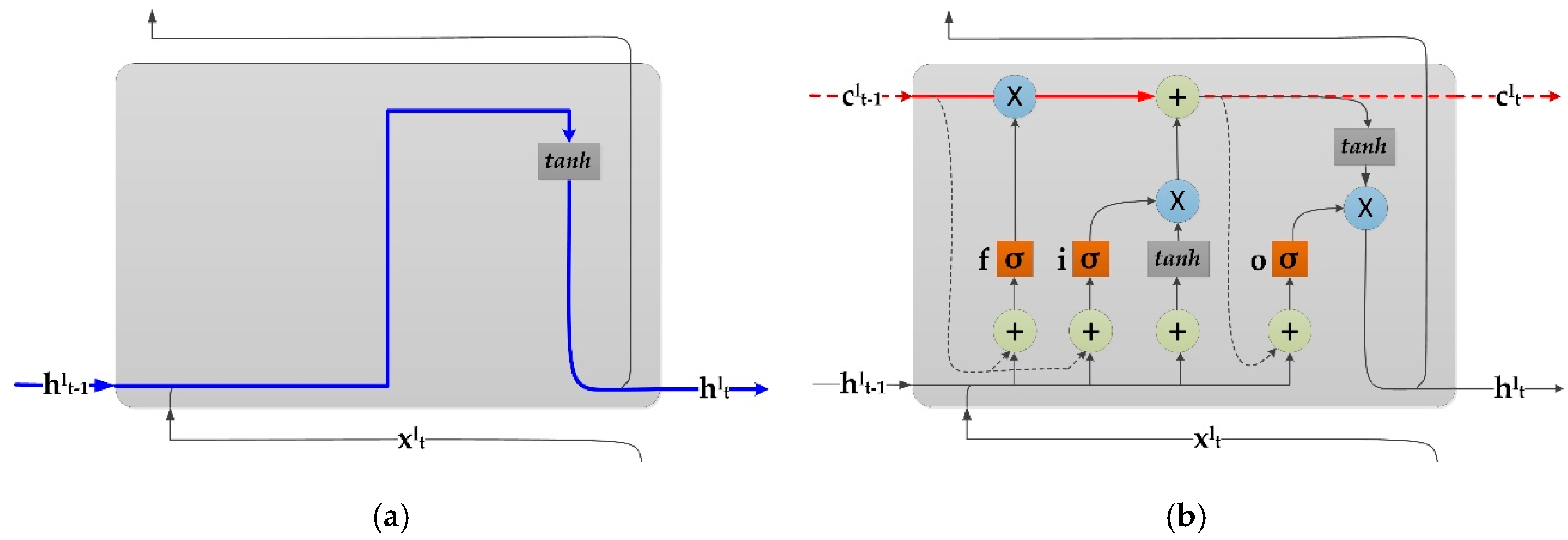
3.1. Long Short-Term Memory RNNs

Due to the long-term correlation of the speech signal, the recurrent neural network is more suitable for completing the speech recognition modeling task than the conventional DNN. The RNN adds a feedback connection to the hidden layer. That is to say, part of the input of the RNN hidden layer at the current moment is the hidden layer output of the previous moment, which allows the RNN to obtain information of all previous moments through the recurrent feedback connection, and it gives RNN memory.
However, the information of RNN can only be passed to the neighboring successors. When the output is close to the relevant input information, an ordinary RNN can be competent. When this time interval is very long, although theoretically RNN can handle this long-term dependence problem, it has not been successful in practice. Hochreiter et al. [22] and others conducted an in-depth study of the problem. They found that the fundamental reason for making RNN training difficult is the vanishing gradient and gradient explosion problem. Therefore, Hochreiter & Schmidhuber [23] proposed a long short-term memory recurrent neural network, which was recently improved and promoted by Alex Graves [11,24,25].
The LSTM maintains the error at a more constant level through a specific gating unit, allowing the RNN to learn multiple time steps, thereby avoiding the vanishing gradient. The LSTM stores information in gated units outside the normal flow of the recurrent neural network. These units can store, write, or read information, just like data in the computer’s memory. The unit determines which information is stored by the switch of the door and when it is allowed to read, write or clear the information. However, unlike digital memories in computers, these gates are analog and contain element-by-element multiplication of sigmoid functions whose output ranges are all between 0 and 1. When compared to digital storage, analog values have the advantage of being differentiable. So it is suitable for back propagation. These gates switch on the basis of the received signal. Similar to the nodes of the neural network, they use their own set of weights to filter the information and decide whether to allow the information to pass based on their strength and the content of the import. These weights, like the weights of modulation inputs and hidden states, are adjusted through the learning process of a recurrent neural network. The memory unit learns when to allow data to enter, leave, or be deleted by an iterative process in which the error propagates back and the weights are adjusted by gradient descent.
A graphical comparison between RNN blocks and LSTM blocks is shown in Figure 1. The LSTM block consists of a set of memory cells c and three gates: input gate i, forget gate f, and output gate o, which are used to control the flow of information.
The following is a brief description of several gating units:
  • Memory unit c: they store the network’s time status;
  • Input gates i: they decide whether to pass input information into cell c;
  • Output gate o: they decide whether to output the cell information; and,
  • Forget gate f: These gates adaptively reset the cell state.
At the time step t, the formula of the LSTM block can be described, as follows:
i t l = σ ( W i l x t l + V i l h t 1 l + U i l c t 1 l + b i l ) f t l = σ ( W f l x t l + V f l h t 1 l + U f l c t 1 l + b f l ) c ^ t l = t a n h ( W c l x t l + V c l h t 1 l + b c l ) c t l = f t l c t 1 l + i t l c ^ t l o t l = σ ( W o l x t l + V o l h t 1 l + U o l c t l + b o l ) h t l = W p r o j l ( o t l t a n h ( c t l ) )
c t l and h t l are, respectively, the cell state and cell output of the first layer at time t; in particular, the cell output h t 0 of layer 0 at time t refers to the input feature vector at time t. W, V, U, and b, respectively, represent the weight matrix and the bias vector connecting different gates. For example, W denotes the weight matrix between input and each gating unit; V denotes the weight matrix between output and each gating unit; U denotes the weight matrix between the cell state to each gating unit. Since only one cell is set for every LSTM block, so U is a diagonal matrix here, and b is a bias vector. σ is a sigmoid activation function. ◦ denotes an element-wise product. As described in [15], W proj l represents a projection matrix.

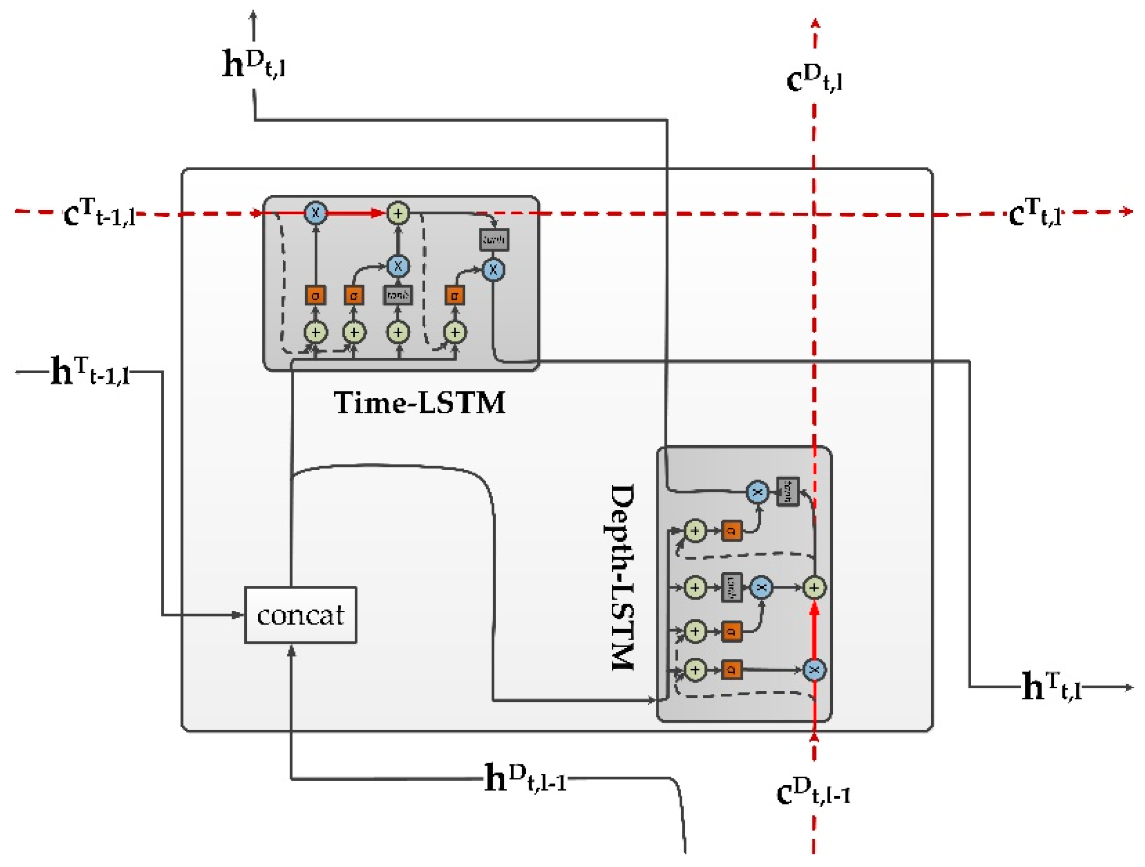
3.2. Grid Long Short-Term Memory RNNs

GridLSTM was first proposed in [9] in 2015, which is an improved structure of the LSTM recurrent neural network. Subsequently, Wei-Ning Hsu and Yu Zhang et al. [20] applied GridLSTM to the field of speech recognition and achieved better recognition results. GridLSTM adopts a method of arranging LSTM blocks into a multidimensional grid, providing a unified framework for depth and timing calculations, and making each dimension in each grid correspond to a series of LSTM blocks. GridLSTM is linearly related to the gating between adjacent cells in each dimension, which makes it possible to mitigate the vanishing gradient in each dimension. As shown in Figure 2, this article uses two-dimensional GridLSTM models for acoustic modeling, in which each grid contains a Depth-LSTM block for depth calculations and a Time-LSTM block for time calculations, respectively.
  • The calculation process of Time-LSTM block is as follows:
    i t , l T = σ ( W i , l D h t , l 1 D + V i , l T h t 1 , l T + U i , l T c t 1 , l T + b i , l T ) f t , l T = σ ( W f , l D h t , l 1 D + V f , l T h t 1 , l T + U f , l T c t 1 , l T + b f , l T ) c ^ t , l T = t a n h ( W c , l D h t , l 1 D + V c , l T h t 1 , l T + b c , l T ) c t , l T = f t , l T c t 1 , l T + i t , l T c ^ t , l T o t , l T = σ ( W o , l D h t , l 1 D + V o , l T h t 1 , l T + U o , l T c t , l T + b o T ) h t , l T = W proj , l T ( o t , l T t a n h ( c t , l T ) )
  • The calculation process of Depth-LSTM block is as follows:
    i t , l D = σ ( W i , l D h t , l 1 D + V i , l T h t 1 , l T + U i , l D c t , l 1 D + b i , l D ) f t , l D = σ ( W f , l D h t , l 1 D + V f , l T h t 1 , l T + U f , l D c t , l 1 D + b f , l D ) c ^ t , l D = t a n h ( W c , l D h t , l 1 D + V c , l T h t 1 , l T + b c , l D ) c t , l D = f t , l D c t , l 1 D + i t , l D c ^ t , l D o t , l D = σ ( W o , l D h t , l 1 D + V o , l T h t 1 , l T + U o , l D c t , l D + b o , l D ) h t , l D = W p r o j , l D ( o t , l D t a n h ( c t , l D ) )
In Equations (2) and (3), we use the superscript T and D to represent the Time-LSTM block in the time dimension and the Depth-LSTM block in the depth dimension; the subscript t represents time, and the l represents the number of layers or depth. For example, c t , l D denotes the cell state of Depth-LSTM in the depth dimension of the first layer at the time t and h t , l T denotes the cell state of Time-LSTM in the time dimension of the first layer at time t. W represents the weight between the output of the Depth-LSTM block in the upper layer grid and each gating unit, and V represents the weight between the output of Time-LSTM at the previous moment and the gating unit in the grid. U represents the weight between the cell states of the LSTM blocks in each dimension of the neighboring grid. In this paper, the initial value of c t , 0 D is set to zero.

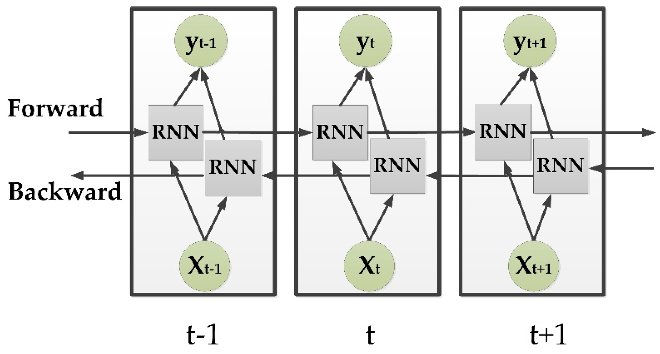
3.3. Bidirectional RNNs

Bidirectional Recurrent Neural Networks (BiRNN) [26] are made up by two separate recurrent hidden layers that scan the input sequence in the opposite direction. The two hidden layers are connected to the same output layer, so the context information can be accessed in two opposite directions. The context information actually used by the network is learned during network training and it does not need to be specified in advance. Therefore, contexts are learnt independently of each other. This point has been elaborated in [27]. Figure 3 shows the structure of a simple bidirectional recurrent neural network.
The BiRNN forward process is the same as the unidirectional RNN. The hidden layer at the time t of the forward RNN is affected by the hidden layer at time t − 1 of the forward RNN and the input x(t) at time t. The hidden layer at time t of the reverse RNN is affected by the t + 1 hidden layer of the reverse RNN and the input x(t) at time t.The RNNs in two different directions do not share the cell state value. The status value of the cell output by the forward RNN is only transmitted to the forward RNN. Similarly, the status value of cell output by the reverse RNN is only transmitted to the reverse RNN. The forward and reverse RNNs are not directly connected.
The input of each time node is respectively transmitted to the forward and reverse RNNs. During the specific calculation, BiRNN first scans the entire sequence. It calculates the hidden state of the forward RNN along the direction from 1 to T, and it then calculates the hidden state of the reverse RNN from T to 1. According to their internal states to output, the forward and reverse outputs are combined and connected to the BiRNN output nodes to synthesize the final output. The current time node loss value is calculated during training. The reverse transmission process of BiRNN is similar to that of RNN, which is trained by the Back Propagation Through Time (BPTT) algorithm [28]. The algorithm first calculates the error of the output layer, and then respectively passes the error along T to 1 and 1 to T to the hidden layers of the forward and reverse RNN, and the model parameters are optimized to the appropriate values, according to the gradient.

3.4. Vanishing Gradient and Context-Sensitivity

LSTM uses the gating unit to overcome the drawbacks of the traditional RNN not being able to memorize long-term information on the time axis. Regrettably, the LSTM still inevitably has the problem of vanishing gradient in the depth direction. As explained in [16], verified with an automatic speech recognition task on the AMI dataset, the LSTM recognition rate drops sharply when the number of network layers increased from three to eight layers. Only the information before the current time has an impact on the output of the LSTM current time point, which is far from enough for the time sequence task. GridLSTM adds a Depth-LSTM block in the depth dimension and encapsulates it with a Time-LSTM block in the time dimension in a grid, trying to solve the gradient problem in both time and depth dimensions. In the GridLSTM time dimension, the current time hidden layer of Time-LSTM is affected by the hidden layer of the previous moment and current time input. Therefore, only the information before the current time can be obtained, but the context-dependent characteristics of the timed task are ignored. However, the output of the time sequence task is affected by the context information, which makes the output more accurate with the content of the moments before and after. The bidirectional RNN uses two separate recurrent hidden layers to scan the input sequence in opposite direction, overcoming the shortcomings of GridLSTM not being able to take advantage of the context information. The RNN in each direction of the bidirectional RNN has the same disadvantages as the normal unidirectional RNN and LSTM. As the number of layers is deepened to a certain extent, the depth dimension will have a phenomenon of vanishing gradient or gradient explosion.

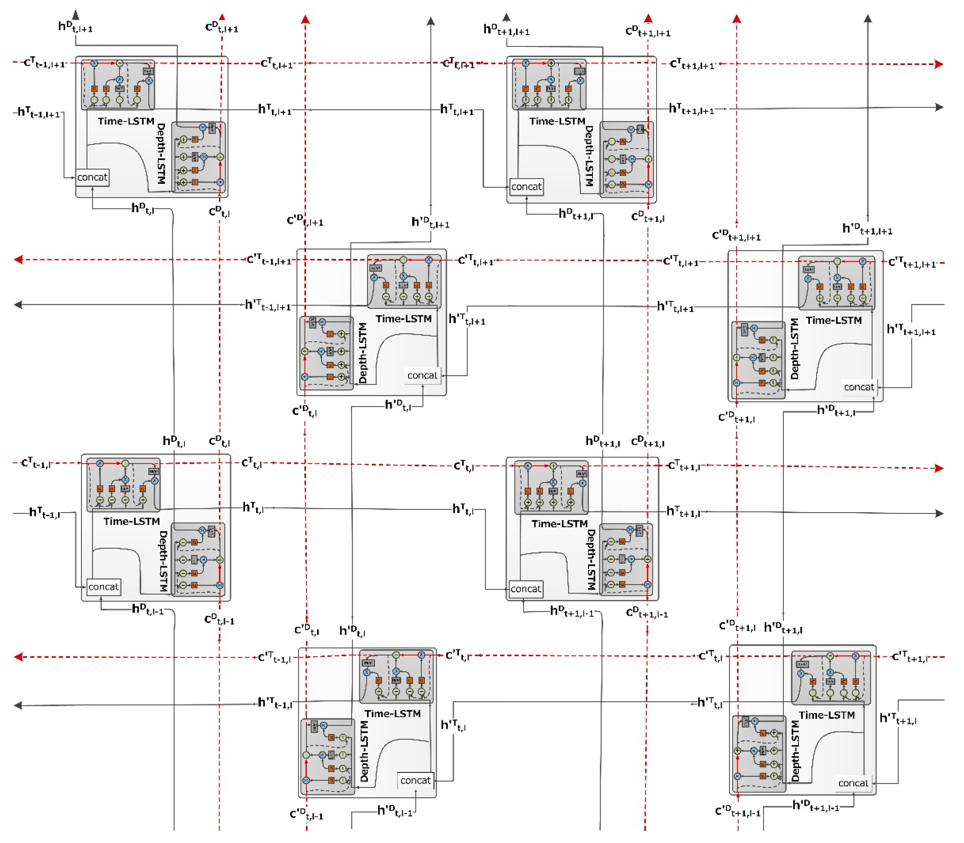
3.5. Bidirectional Grid Long Short-Term Memory RNNs

As shown in Figure 4, BiGridLSTM is a recurrent neural network architecture that combines LSTM with grid architecture and bidirectional architecture. BiGridLSTM consists of two GridLSTM recurrent neural networks in the opposite direction. Each GridLSTM contains two LSTM blocks, Time-LSTM and Depth-LSTM. Each LSTM block is composed of an input gate, a forget gate, an output gate and a memory unit, which are used to control the flow of information, determine whether to allow the flow of information to pass, output or forget, and when to allow reading, writing, or clearing information according to the gate switch. The hidden layer output of the forward GridLSTM is similar to the output of a normal RNN, which consists of the input of the current moment and the output of the previous moment. The outputs of the hidden layer 1 at the time t in the depth direction and the time dimension are affected by the output h t 1 , l T of the hidden layer 1 at the time t − 1 in the time dimension and the input x D ( t ) at time t in the depth direction or output h t 1 , l D of the hidden layer l − 1 at the time t in the forward GridLSTM. Similarly, the outputs of the hidden layer 1 at the time t in the depth direction and the time dimension are affected by the output h t + 1 , l T of the hidden layer 1 at the time t + 1 in the time dimension and the input x D ( t ) at time t in the depth direction or output h t , l 1 D of the hidden layer l − 1 at the time t in the reverse GridLSTM. The outputs of forward and reverse GridLSTM are combined and connected to the output nodes to form the final output of BiGridLSTM. It is worth noting that the GridLSTM does not share the cell state in two different directions. The cell state values of the outputs by the Time-LSTM and Depth-LSTM blocks in forward GridLSTM are only passed to the Time-LSTM and Depth-LSTM blocks of the forward GridLSTM, and the cell status values of the outputs by the Time-LSTM and Depth-LSTM blocks in reverse GridLSTM are only passed to the Time-LSTM and Depth-LSTM blocks of the reverse GridLSTM. Moreover, the forward and reverse GridLSTM are not directly connected.
On the one hand, BiGridLSTM increases the cell state flow in both time and depth, which makes this structure address the problem that RNN can not get remote information and alleviate the vanishing gradient in vertical dimension as mentioned in Section 3.1 above [22]. On the other hand, BiGridLSTM uses the forward and reverse GridLSTM to scan the input sequence together, which makes it overcome the drawbacks of not being able to capture context information at the same time. In this paper, we verify the BiGridLSTM model in the speech recognition task. When compared with other unidirectional models and deep models, the performance can be greatly improved.
  • The simplified formulas for the Time-LSTM and Depth-LSTM in the forward GridLSTM block are defined, as follows:
    ( h t , l T , c t , l T ) = T I M E - L S T M ( h t , l 1 D , h t 1 , l T , c t 1 , l T , Θ T ) ( h t , l D , c t , l D ) = D E P T H - L S T M ( h t , l 1 D , h t 1 , l T , c t , l 1 D , Θ D )
  • The simplified formulas for the T-LSTM and D-LSTM in the reverse GridLSTM block are defined, as follows:
    ( h t , l T , c t , l T ) = T I M E - L S T M ( h t , l 1 D , h t + 1 , l T , c t + 1 , l T , Θ T ) ( h t , l D , c t , l D ) = D E P T H - L S T M ( h t , l 1 D , h t + 1 , l T , c t , l 1 D , Θ D )
Finally, the combined total output of the forward and reverse GridLSTM is:
y t , l = Grid L S T M ( h t , l D , h t , l D )
In Equations (4)–(6), the symbol “→” indicates the forward GridLSTM block. The symbol “←” indicates the reverse GridLSTM block. The symbol “Θi” stands for all the parameters in the i-LSTM block. yt,l indicates the total output of hidden layer l at time t. The cell outputs h t , l D of the last layer Depth-LSTM as input to the fully connected layer. In addition, the cell state initial value c t , 0 D of the first layer Depth-LSTM is initialized to zero.

4. Experiment Setup

4.1. Dataset

This paper will validate our BiGridLSTM model on speech recognition tasks, all of which are done on the LibriSpeech corpus. LibriSpeech is a corpus of approximately 1000 h of English speech that was recorded at a sampling rate of 16 kHz by Vassil Panayotov with the assistance of Daniel Povey. These data come from the audio books of the LibriVox project and they are carefully classified and aligned. According to the description in [29], the training set of corpus is divided into three subsets, approximately 100, 360 and 500 h, respectively. Speakers in the corpus are ranked according to the WER of the WSJ model transcripts and they are roughly divided in the middle. Speakers with lower WER are designated as “clean” and speakers with higher WER are designated as “other”. Randomly selected 20 men and 20 female speakers from the “clean” data set were assigned to a development set. Repeat the same steps to form a test set. For each development set or test set speaker, approximately 8 min of speech is used, for a total of approximately 5 h and 20 min. Our systems follow the split that is recommended in the corpus release: 100 h, 5.3 h, 5.3 h for training, validation, and test set designated as “clean”, respectively.

4.2. Metrics

This paper will use Sensitivity, Specificity, F-measure and CER as metrics to judge the speech recognition performance. To help with the analysis, we define the following symbols:
C = Number   of   correctly   recognized   characters S = Number   of   substitutions I = Number   of   insertions D = Number   of   Deletions
1. CER
The CER (character error rate) is a metrics that compares the character sequence that is obtained by the model with the actually transcribed character sequence. In this paper, the recognition performance of the model is measured by the character error rate calculated by the edit distance. The edit distance is a quantitative measure of the degree of difference between two strings. The measurement method refers to how many edit operations are required to change one string to another. Allowed editing operations include replacing one character with another, inserting one character, and deleting one character. The CER calculation formula is as follows:
CER = S + I + D C + S + I + D
2. F-measure
F-measure is a weighted harmonic average of precision and recall. It is a comprehensive evaluation indicator for evaluating the performance of the model. In speech recognition, the precision rate is the ratio of the number of correctly recognized characters to the sum of the number of correctly recognized, replaced, and inserted characters. The recall rate is the ratio of the number of correctly recognized characters to the sum of the number of correctly recognized, replaced, and deleted characters. We use the following formula to calculate the precision rate, recall rate, and F-Measure:
Precision = C C + S + I Recall = C C + S + D F - Measure = a 2 + 1 1 Precision + a 2 Recall
When a = 1, it is the most commonly used F1. In this paper, F1 is used as a comprehensive indicator of the precision and recall rate to judge the speech recognition performance
F 1 = 2 × Precision × Recall Precision + Recall
3. Sensitivity
Sensitivity refers to the true positive rate, which is similar to the recall rate. Sensitivity can be used to measure the ability to identify the correct character in a speech recognition task. Sensitivity is the ratio of the number of correctly recognized characters to the sum of the number of correctly recognized, replaced, and deleted characters. It can be defined by the following formula:
Sensitivity = C C + S + D
4. Specificity
Specificity refers to the true negative rate. It can be defined by the following formula:
Specificity = C + D I C + S + D

4.3. Model Setup

We use models, such as LSTM, GRU, and GridLSTM as baseline models here. The baseline model contains 512 memory cells per layer and adds a 512-node linear projection layer at each layer output. The baseline models LSTM and GridLSTM will be used for the first three experiments, while the GRU will be used only in the first two experiments. For our unidirectional and bidirectional grid LSTM models (UniGridLSTM/BiGridLSTM) we chose the same time LSTM and deep LSTM configuration as the above baseline model. Other model configurations will be described in the fifth chapter.

4.4. Preprocessing and Training

A typical ASR feature extraction process is roughly divided into frames, windows, Fourier transforms, Mel filters, logarithms, and the final discrete cosine transform DCT [30]. In this paper, the speech signal is divided into 40 frames per second, 25 ms per frame, and adjacent frames overlap 10 ms. Each frame of speech signal is transformed into a spectrogram through 512 Fast Fourier Transforms (FFTs), and is then converted to a mel spectrum by 26 mel filters. The cepstrum analysis of the mel cepstral is then performed to obtain the mel-frequency cepstrum coefficient, which is represented by a 13-dimensional vector. Then, the first derivative and second derivative of the Mel frequency cepstrum coefficients are obtained, and finally they are merged into a 39-dimensional mel spectrum vector.
All experiments will be conducted using the TensorFlow [31] framework, which allows for us to efficiently build and evaluate various network structures without extending and implementing complex training algorithms. As suggested by [32], this paper selects the dynamic recurrent neural network tf.nn.dynamic_rnn to construct the recurrent neural network and solves the memory and sequence length limitation by using the tf.while loop to dynamically expand the graph during execution. This means that the chart is created faster and the batch can have a variable sequence length. A fully connected layer with 512 hidden units is added to the output of the recurrent neural layer for the classification of phonetic characters. In general, the weight initialization method should ensure that the weight is close to 0 and it is not too small. Truncated normal distribution will cut off values outside twice the standard deviation, which is equivalent to discarding values farther away from 0, making most of them close to 0. Therefore, the weights are all randomly initialized from the truncated uniform normal distribution, and all biases are initialized to zero [33]. Unless otherwise specified, all neural network models use the loss function tf.nn.ctc_loss [34], which is connectionist temporal classification loss function and commonly used in speech recognition, to train the neural network acoustic model so that no manual alignment of speech and text is required. Then, the Adam optimizer dynamically adjusts the learning rate for each parameter based on the first moment estimation and second moment estimation of the loss function gradient for each parameter, the initial learning rate is set to 0.001. Adam also uses BPTT for optimization, but the learning step size for each iteration parameter has a definite range. It does not result in a large learning step because of the large gradient, and the value of the parameter is relatively stable. In addition, in order to avoid vanishing gradient and gradient explosion, gradient clipping is used in the weight updating process to limit the updating of weights in a suitable range. Finally, the decoding operation is performed while using tf.nn.ctc_beam_search_decoder, which outputs a list of probabilities, and the maximum probability value is selected as the final recognition result. The core algorithm used in the decoding process is beam search, which uses a greedy strategy.

5. Results and Discussion

All of the experiments in this paper will be performed on the LibriSpeech corpus, and the character error rate (CER), F1 value, Sensitivity and Specificity on the test set are the criterion for judging the accuracy of speech recognition.

5.1. Grid LSTM Model and Baseline

We first compared the GridLSTM and other baseline models on the train-clean-100 dataset in the LibriSpeech corpus. In this experiment, each loop layer was set to two layers, and the output layer was a fully connected layer. The speech recognition evaluation indicators of different models are shown in Table 1. GridLSTM has the lowest CER on the LibriSpeech corpus and the highest comprehensive index F1. The sensitivity and specificity values of GridLSTM are larger than other models. Specifically, when compared to LSTM, the CER of GridLSTM can achieve a relative gain of 5.55%. In addition, it can be seen that the LSTM speech recognition task on the LibriSpeech corpus is more advantageous than the LSTM variant GRU. The results show that the GridLSTM model better exploits the benefits of introducing gated linear dependence across depth dimensions. This result is consistent with the results in [20].

5.2. Unidirectional/Bidirectional Grid LSTM

Next, we verify the effect of BiGridLSTM on the character error rate. In order to separate the influence between the bidirectional structure and depth, we only compare the bidirectional models with two layers of recurrent layers.
Table 2 shows that by introducing a bidirectional structure, all bidirectional model CERs are lower than that of their unidirectional models, and F1 value is higher. It is verified that the bidirectional structure can capture the information before and after the current moment. Surprisingly, BiGridLSTM achieves a relative gain of approximately 26% in their CER as compared to unidirectional GridLSTM, which demonstrates the validity of our proposed model. It is worth noting that the bidirectional grid LSTM has more gain than the bidirectional LSTM and the bidirectional GRU, and has higher sensitivity and specificity. Therefore, it is demonstrated that with the bidirectional structure, the grid LSTM can further reduce the CER of speech recognition on the LibriSpeech corpus, and improve the sensitivity and specificity of the model. More discussion is found in Section 5.3.

5.3. Comparisons with Alternative Deep LSTM

We studied the effect of three models that increase the depth of the network on the LibriSpeech corpus. Table 3 summarizes the results of the deep models as compared to the baseline. When increasing the number of layers, the neural network usually encounters the well known vanishing gradient problem, just as we can observe from the test results of the LSTM model. As described in [4], the grid LSTM model can mitigate the vanishing gradient problem and thus can train deeper models. From the experimental results, it can be seen that when the number of layers of GridLSTM and BiGridLSTM is increased from 2 to 5, the character error rate is reduced by about 12%, and F1 values, sensitivity, and specificity are increased, indicating that both GridLSTM and BiGridLSTM will benefit from increasing the depth.
It is worth noting that the accuracy of the 2-layer BiGridLSTM model is higher than that of the 5-layer GridLSTM model. The 2-layer BiGridLSTM has a shorter training time and consumes less memory space. We believe that it is a crucial factor to use the LSTM bidirectional structure to obtain contextual information for good performance. In addition, as compared to the two-layer BiridGLSTM with 256 hidden layer units, the five-layer BiGridLSTM reduces the CER by 12.68% with the hidden layer unit reduced to 128. In summary, the bidirectional grid LSTM further reduces the speech recognition CER, and improves model sensitivity and specificity as the number of layers increases, thereby alleviating the gradient problem during training.

5.4. Deeper Bidirectional Grid LSTM

In this section, we built a bidirectional grid LSTM model with eight loop layers, and the number of hidden layer units per hidden layer was reduced to 128. Table 4 shows the comparison results with the two-layer and five-layer BiGridLSTM. However, BiGridLSTM does not deteriorate performance due to the vanishing gradients as the number of layers deepens. As we assumed, it benefits from increasing the number of layers. This result also supports the hypothesis that BiGridLSTM provides more flexibility in selecting the number of model layers.

6. Conclusions

In this paper, we propose a comprehensive study of the grid LSTM and the bidirectional recurrent structure. By taking advantage of these two strategies, we propose a novel architecture, called BiGridLSTM, which solves the gradient problems by constructing a unified framework for depth and time calculations and introducing gated linear correlations between neighboring cells in each layer of each dimension. In addition, it adds the bidirectional structure in the recurrent layer to obtain context information at the current moment. We validated our BiGridLSTM model by performing a speech recognition task on the train-clean-100 data set of the English audio book LibriSpeech. The results show that our BiGridLSTM model outperforms all of the baseline models in the paper, and verify the assumption that using bidirectional structures to obtain contextual information is critical to achieving good performance. At the same time, the reduced CER can help completing structured and free-text queries on transcribed speech more accurately, which benefits the Semantic Web.
For future work, on the one hand, we plan to add priority features to the bidirectional grid LSTM model; on the other hand, we combine time-frequency LSTM with bidirectional grid LSTM to improve the model recognition performance. We also want to study more in-depth models in larger tasks, such as large vocabulary speech recognition, machine translation, stock forecasting, and behavior recognition, etc.

Author Contributions

H.F. and F.T. proposed innovative idea; F.T. conceived the design of the solution, and wrote the first draft; F.T. worked on the implementation and improvement of the model; H.F. and F.T. verified the effect of the model; F.T. wrote the later versions of the paper; H.F. supervised the paperwork and provided writing advice; H.F. provided feasibility advice and hardware support.

Funding

This research received no external funding.

Conflicts of Interest

The authors declare no conflict of interest.

References

  1. Graves, A.; Mohamed, A.R.; Hinton, G. Speech Recognition with Deep Recurrent Neural Networks. In Proceedings of the IEEE International Conference on Acoustics, Speech and Signal Processing(ICASSP), Vancouver, BC, Canada, 26–30 May 2013; Volume 38, pp. 6645–6649. [Google Scholar]
  2. Li, B.; Sim, K.C. Modeling long temporal contexts for robust DNN-based speech recognition. In Proceedings of the Fifteenth Annual Conference of the International Speech Communication Association, Singapore, 7–10 September 2014. [Google Scholar]
  3. Li, J.; Mohamed, A.; Zweig, G.; Gong, Y. Exploring Multidimensional LSTMs for Large Vocabulary ASR. In Proceedings of the IEEE International Conference on Acoustics Speech and Signal Processing(ICASSP), Shanghai, China, 20–25 March 2016; pp. 4940–4944. [Google Scholar]
  4. Yu, D.; Li, J. Recent progresses in deep learning based acoustic models. IEEE J. 2017, 4, 396–409. [Google Scholar] [CrossRef]
  5. Hinton, G.E.; Geoffrey, E.; Salakhutdinov, R.R. Reducing the dimensionality of data with neural networks. Science 2006, 313, 504–507. [Google Scholar] [CrossRef] [PubMed]
  6. Zhao, M.; Kang, M.; Tang, B.; Pecht, M. Deep Residual Networks With Dynamically Weighted Wavelet Coefficients for Fault Diagnosis of Planetary Gearboxes. IEEE Trans. Ind. Electron. 2018, 65, 4290–4300. [Google Scholar] [CrossRef]
  7. Dey, R.; Salemt, F.M. Gate-variants of Gated Recurrent Unit (GRU) neural networks. In Proceedings of the 60th IEEE International Midwest Symposium on Circuits and Systems, Boston, MI, USA, 6–9 August 2017; pp. 1597–1600. [Google Scholar]
  8. Chung, J.; Gulcehre, C.; Cho, K.H.; Bengio, Y. Empirical Evaluation of Gated Recurrent Neural Networks on Sequence Modeling. arXiv, 2014; arXiv:1412.3555. [Google Scholar]
  9. Kalchbrenner, N.; Danihelka, I.; Graves, A. Grid long short-term memory. arXiv, 2015; arXiv:1507.01526. [Google Scholar]
  10. Graves, A.; Schmidhuber, J. Framewise phoneme classification with bidirectional LSTM networks. In Proceedings of the IEEE International Joint Conference on Neural Networks(IJCNN), Montreal, QC, Canada, 31 July–4 August 2005; Volume 4, pp. 2047–2052. [Google Scholar]
  11. Graves, A.; Jaitly, N.; Mohamed, A.R. Hybrid Speech Recognition with Deep Bidirectional LSTM. In Proceedings of the IEEE Automatic Speech Recognition and Understanding (ASRU), Olomouc, Czech Republic, 8–12 December 2013; pp. 273–278. [Google Scholar]
  12. Chiu, J.P.C.; Nichols, E. Named Entity Recognition with Bidirectional LSTM-CNNs. arXiv, 2015; arXiv:1511.08308. [Google Scholar]
  13. Huang, Z.; Xu, W.Y.K. Bidirectional LSTM-CRF Models for Sequence Tagging. arXiv, 2015; arXiv:1508.01991. [Google Scholar]
  14. Panayotov, V.; Chen, G.; Povey, D.; Khudanpur, S. Librispeech: An ASR Corpus Based on Public Domain Audio Books. In Proceedings of the IEEE International Conference on Acoustics, Speech and Signal Processing (ICASSP), Brisbane, Australia, 19–24 April 2015; pp. 5206–5210. [Google Scholar]
  15. Sak, H.; Senior, A.; Beaufays, F. Long short-term memory recurrent neural network architectures for large scale acoustic modeling. In Proceedings of the 15th Annual Conference of the International Speech Communication Association (INTERSPEECH), Singapore, 7–10 September 2014; pp. 338–342. [Google Scholar]
  16. Zhang, Y.; Chen, G.; Yu, D.; Yaco, K.; Khudanpur, S.; Glass, J. Highway long short-term memory RNNs for distant speech recognition. In Proceedings of the IEEE International Conference on Acoustics, Speech and Signal Processing (ICASSP), Shanghai, China, 20–25 March 2016; pp. 5755–5759. [Google Scholar]
  17. Kim, J.; Elkhamy, M.; Lee, J. Residual LSTM: Design of a deep recurrent architecture for distant speech recognition. arXiv, 2017; arXiv:1701.03360. [Google Scholar]
  18. Zhao, Y.; Xu, S.; Xu, B. Multidimensional Residual Learning Based on Recurrent Neural Networks for Acoustic Modeling. In Proceedings of the 17th Annual Conference of the International Speech Communication Association (INTERSPEECH), San Francisco, CA, USA, 8–12 September 2016; pp. 3419–3423. [Google Scholar]
  19. He, K.; Zhang, X.; Ren, S.; Sun, J. Deep residual learning for image recognition. In Proceedings of the IEEE International Conference on Computer Vision and Pattern Recognition (CVPR), Las Vegas, NV, USA, 26 June–1 July 2016; pp. 770–778. [Google Scholar]
  20. Hsu, W.N.; Zhang, Y.; Glass, J. A prioritized grid long short-term memory RNN for speech recognition. In Proceedings of the IEEE Workshop on Spoken Language Technology (SLT), San Diego, CA, USA, 13–16 December 2016; pp. 467–473. [Google Scholar]
  21. Kreyssing, F.; Zhang, C.; Woodland, P. Improved TDNNs using Deep Kernels and Frequency Dependent Grid-RNNs. In Proceedings of the IEEE International Conference on Acoustics, Speech and Signal Processing(ICASSP), Calgary, AB, Canada, 15–20 April 2018; pp. 1–5. [Google Scholar]
  22. Hochreiter, S. Untersuchungen zu Dynamischen Neuronalen Netzen. Master’s Thesis, Munich Industrial University, Munich, Germany, 1991. [Google Scholar]
  23. Graves, A. Long Short-Term Memory; Springer: Berlin, Germany, 2012; pp. 1735–1780. [Google Scholar]
  24. Graves, A.; Jaitly, N. Towards end-to-end speech recognition with recurrent neural networks. In Proceedings of the International Conference on Machine Learning (ICML), Beijing, China, 22–24 June 2014; pp. 1764–1772. [Google Scholar]
  25. Graves, A. Generating sequences with recurrent neural networks. arXiv, 2013; arXiv:1308.0850. [Google Scholar]
  26. Schuster, M.; Paliwal, K.K. Bidirectional recurrent neural networks. IEEE Trans. Signal. Process. 2002, 45, 2673–2681. [Google Scholar] [CrossRef]
  27. Wöllmer, M.; Eyben, F.; Graves, A.; Schuller, B.; Rigoll, G. Bidirectional LSTM Networks for Context-Sensitive Keyword Detection in a Cognitive Virtual Agent Framework. Cognit. Comput. 2010, 2, 180–190. [Google Scholar] [CrossRef] [Green Version]
  28. Williams, R.J.; Peng, J. An Efficient Gradient-Based Algorithm for On-Line Training of Recurrent Network Trajectories. Neural Comput. 1990, 2, 490–501. [Google Scholar] [CrossRef]
  29. Panayotov, V.; Chen, G.; Povey, D.; Khudanpur, S. Speech Recognition with Deep Recurrent Neural Networks. In Proceedings of the IEEE International Conference on Acoustics, Speech and Signal Processing (ICASSP), Brisbane, Australia, 19–24 April 2015; pp. 5206–5210. [Google Scholar]
  30. Hossan, M.A.; Gregory, M.A. Speaker recognition utilizing distributed DCT-II based mel frequency cepstral coefficients and fuzzy vector quantization. Int. J. Speech Technol. 2013, 16, 103–113. [Google Scholar] [CrossRef]
  31. Graves, A.; Mohamed, A.R.; Hinton, G. Tensorflow: A system for large-scale machine learning. In Proceedings of the 12th USENIX Symposium on Operating Systems Design and Implementation (OSDI), Savannah, GA, USA, 2–4 November 2016; pp. 256–283. [Google Scholar]
  32. Variani, E.; Bagby, T.; Mcdermott, E.; Bacchiani, M. End-to-end training of acoustic models for large vocabulary continuous speech recognition with tensorflow. In Proceedings of the 18th Annual Conference of the International Speech Communication Association (INTERSPEECH), Stockholm, Sweden, 20–24 August 2017; pp. 1641–1645. [Google Scholar]
  33. Seide, F.; Li, G.; Chen, X.; Yu, D. Feature engineering in context-dependent deep neural networks for conversational speech transcription. In Proceedings of the IEEE Workshop on Automatic Speech Recognition and Understanding (ASRU), Waikoloa, HI, USA, 11–15 December 2011; pp. 24–29. [Google Scholar]
  34. Graves, A.; Gomez, F. Connectionist temporal classification: Labelling unsegmented sequence data with recurrent neural networks. Int. Conf. Mach. Learn. 2006, 2006, 369–376. [Google Scholar]
Figure 1. A comparison between Recurrent Neural Network (RNN) and Long Short-Term Memory (LSTM) blocks. (a) The internal structure of the RNN block. The bold blue line indicates that RNN blocks store memories in the form of hidden state activation. (b) The internal structure of the LSTM block. Dashed lines indicate peephole connections. The bold red line denotes that the LSTM block retains memories in the form of memory cell states, and memory cell states across two consecutive time steps are linearly related by the gating unit.
Algorithms 11 00172 g001
Figure 2. GridLSTM (GridLSTM) blocks. A GridLSTM block contains two LSTM blocks in different dimensions. Time-LSTM denotes the LSTM in the time dimension; Depth-LSTM denotes the LSTM block in the depth dimension.
Algorithms 11 00172 g002
Figure 3. Bidirectional RNN expands in time.
Algorithms 11 00172 g003
Figure 4. Bidirectional Grid LSTM expands in time. Symbol ′ indicates reverse in figure.
Algorithms 11 00172 g004
Table 1. Character error rate (CER) comparison of GridLSTM model and baseline. The bold data in table indicates the minimum CER and highest sensitivity, specificity, and F1 in the experiment.
ModelLayerHidden SizeParamsCER (%)F1 (%)Sensitivity (%)Specificity (%)
LSTM2256835,86921.6479.5080.1178.93
GRU2256628,76524.6276.6877.3876.12
GridLSTM22562,262,81320.4481.0381.4679.78
Table 2. CER comparison of bidirectional models and unidirectional models. The bold data in table indicates the minimum CER and highest sensitivity, specificity, and F1 in the experiment.
ModelLayerHidden SizeParamsCER (%)F1 (%)Sensitivity (%)Specificity (%)
GRU2256628,76524.6276.6877.3876.12
BiGRU22561,250,07718.9382.1082.8981.66
LSTM2256835,86921.6479.5080.1178.93
BiLSTM22561,664,28516.2283.9384.5783.21
GridLSTM22562,262,81320.4481.0381.4679.78
BiGridLSTM22564,518,17315.0685.7786.3085.38
Table 3. CER comparison of deeper models and baseline. The bold data in table indicates the minimum CER and highest sensitivity, specificity, and F1 in the experiment.
ModelLayerHidden SizeParamsCER (%)F1 (%)Sensitivity (%)Specificity (%)
LSTM2256835,86921.6479.5080.1178.93
LSTM52562,411,80521.8579.3779.8078.42
GridLSTM22562,262,81320.4481.0381.4679.78
GridLSTM52565,812,50917.8383.4783.9582.88
BiGridLSTM22564,518,17315.0685.7786.3085.38
BiGridLSTM51282,925,21313.1588.0288.5387.21
Table 4. CER comparison of BiGridLSTM models of different numbers of layers. The bold data in table indicates the minimum CER and highest sensitivity, specificity, and F1 in the experiment.
ModelLayerHidden SizeParamsCER (%)F1 (%)Sensitivity (%)Specificity (%)
BiGridLSTM22564,518,17315.0685.7786.3085.38
BiGridLSTM51282,925,21313.1588.0288.5387.21
BiGridLSTM81284,705,43712.1088.9489.1788.20

