A Faster Algorithm for Reducing the Computational Complexity of Convolutional Neural Networks

Abstract

Convolutional neural networks have achieved remarkable improvements in image and video recognition but incur a heavy computational burden. To reduce the computational complexity of a convolutional neural network, this paper proposes an algorithm based on the Winograd minimal filtering algorithm and Strassen algorithm. Theoretical assessments of the proposed algorithm show that it can dramatically reduce computational complexity. Furthermore, the Visual Geometry Group (VGG) network is employed to evaluate the algorithm in practice. The results show that the proposed algorithm can provide the optimal performance by combining the savings of these two algorithms. It saves 75% of the runtime compared with the conventional algorithm.

1. Introduction

Deep convolutional neural networks have achieved remarkable improvements in image and video processing [1,2,3]. However, the computational complexity of these networks has also increased significantly. Since the prediction process of the networks used in real-time applications requires very low latency, the heavy computational burden is a major problem with these systems. Detecting faces from video imagery is still a challenging task [4,5]. The success of convolutional neural networks in these applications is limited by their heavy computational burden.

There have been a number of studies on accelerating the efficiency of convolutional neural networks. Denil et al. [6] indicate that there are significant redundancies in the parameterizations of neural networks. Han et al. [7] and Guo et al. [8] use certain training strategies to compress these neural network models without significantly weakening their performance. Some researchers [9,10,11] have found that low-precision computation is sufficient for the networks. Binary/Ternary Net [12,13] restricts the parameters to two or three values. Zhang et al. [14] used low-rank approximation to reconstruct the convolution matrix, which can reduce the complexity of convolution. These algorithms are effective in accelerating computation in the network, but they also cause a degradation in accuracy. Fast Fourier Transform (FFT) is also useful in reducing the computational complexity of convolutional neural networks without losing accuracy [15,16], but it is only effective for networks with large kernels. However, convolutional neural networks tend to use small kernels because they achieve better accuracy than networks with larger kernels [1]. For these reasons, there is a demand for an algorithm that can accelerate the efficiency of networks with small kernels.

In this paper, we present an algorithm based on Winograd’s minimal filtering algorithm which was proposed by Toom [17] and Cook [18] and generalized by Winograd [19]. The minimal filtering algorithm can reduce the computational complexity of each convolution in the network without losing accuracy. However, the computational complexity is still large for real-time requirements. To reduce further the computational complexity of these networks, we utilize the Strassen algorithm to reduce the number of convolutions in the network simultaneously. Moreover, we evaluate our algorithm with the Visual Geometry Group (VGG) network. Experimental results show that it can save 75% of the time spent on computation when the batch size is 32.

The rest of this paper is organized as follows. Section 2 reviews related work on convolutional neural networks, the Winograd algorithm and the Strassen algorithm. The proposed algorithm is presented in Section 3. Several simulations are included in Section 4, and the work is concluded in Section 5.

2. Related Work

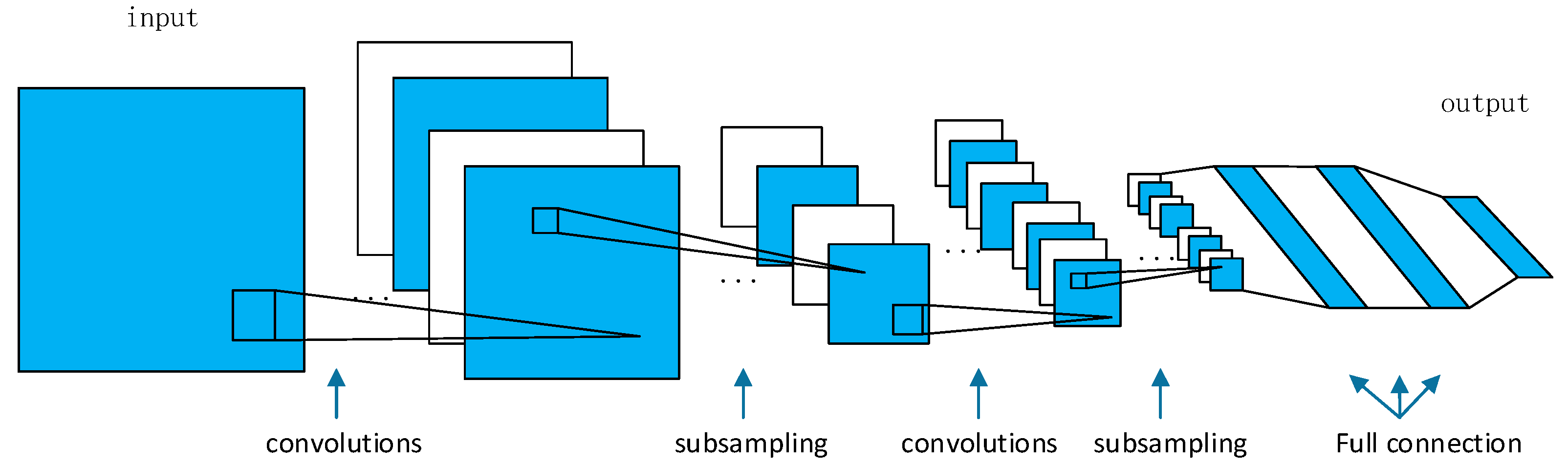
2.1. Convolutional Neural Networks

Machine-learning has produced impressive results in many signal processing applications [20,21]. Convolutional neural networks extend the machine-learning capabilities of neural networks by introducing convolutional layers to the network. Convolutional neural networks are mainly used in image processing. Figure 1 shows the structure of a classical convolutional neural network, LeNet. It consists of two convolutional layers, two subsampling layers and three fully connected layers. Usually, the computation of the convolutional layers occupies most of the network.

Figure 1. The architecture of LeNet.

Convolutional layers extract features from the input feature maps via different kernels. Suppose there are Q input feature maps of size Mx × Nx and R output feature maps of size My × Ny. The size of the convolutional kernel is Mw × Nw. The computation of the output in a single layer is given by the equation

$${\mathrm{y}}_{\mathrm{r},\mathrm{x},\mathrm{y}}={\displaystyle \sum _{\mathrm{q}=1}^{\mathrm{Q}}{\displaystyle \sum _{\mathrm{u}=1}^{\mathrm{Mw}}{\displaystyle \sum _{\mathrm{v}=1}^{\mathrm{Nw}}{\mathrm{w}}_{\mathrm{r},\mathrm{q},\mathrm{u},\mathrm{v}}{\mathrm{x}}_{\mathrm{q},\mathrm{x}+\mathrm{u},\mathrm{y}+\mathrm{v}}}}},$$

(1)

where X is the input feature map, Y is the output feature map, and W is the kernel. The subscripts x and y indicate the position of the pixel in the feature map. The subscripts u and v indicate the position of the parameter in the kernel. Equation (1) can be rewritten as Equation (2).

$${\mathrm{y}}_{\mathrm{r}}={\displaystyle \sum _{\mathrm{q}=1}^{\mathrm{Q}}{\mathrm{w}}_{\mathrm{r},\mathrm{q}}\ast {\mathrm{x}}_{\mathrm{q}}}$$

(2)

Suppose there are P images that are sent together to the neural network, which means the batch size is P. Then the output Y in Equation (2) can be expressed by Equation (3).

$${\mathrm{y}}_{\mathrm{r},\mathrm{p}}={\displaystyle \sum _{\mathrm{q}=1}^{\mathrm{Q}}{\mathrm{w}}_{\mathrm{r},\mathrm{q}}\ast {\mathrm{x}}_{\mathrm{q},\mathrm{p}}}$$

(3)

If we regard the y_r,p, w_r,q and x_q,p as the elements of the matrices Y, W and X, respectively, the output can be expressed as the convolution matrix in Equation (4).

$$\mathrm{Y}=\mathrm{W}\ast \mathrm{X}$$

(4)

$$\mathrm{Y}=\left[\begin{array}{ccc}{\mathrm{y}}_{1,1}& \cdots & {\mathrm{y}}_{1,\mathrm{P}}\\ ⋮& \ddots & ⋮\\ {\mathrm{y}}_{\mathrm{R},1}& \cdots & {\mathrm{y}}_{\mathrm{R},\mathrm{P}}\end{array}\right]\mathrm{W}=\left[\begin{array}{ccc}{\mathrm{w}}_{1,1}& \cdots & {\mathrm{w}}_{1,\mathrm{Q}}\\ ⋮& \ddots & ⋮\\ {\mathrm{w}}_{\mathrm{R},1}& \cdots & {\mathrm{w}}_{\mathrm{R},\mathrm{Q}}\end{array}\right]\mathrm{X}=\left[\begin{array}{ccc}{\mathrm{x}}_{1,1}& \cdots & {\mathrm{x}}_{1,\mathrm{P}}\\ ⋮& \ddots & ⋮\\ {\mathrm{x}}_{\mathrm{Q},1}& \cdots & {\mathrm{x}}_{\mathrm{Q},\mathrm{P}}\end{array}\right]$$

(5)

Matrix Y and matrix X are special matrices of feature maps. Matrix W is a special matrix of kernels. This convolutional matrix provides a new view of the computation of the output Y.

2.2. Winograd Algorithm

We denote an r-tap FIR filter with m outputs as F(m, r). The conventional algorithm for F(2, 3) is shown in Equation (6), where d₀, d₁, d₂ and d₃ are the inputs of the filter, and h₀, h₁ and h₂ are the parameters of the filter. As Equation (6) shows, it uses 6 multiplications and 4 additions to compute F(2, 3).

$$\mathrm{F}(2,3)=\left[\begin{array}{c}\begin{array}{ccc}{\mathrm{d}}_0& {\mathrm{d}}_1& {\mathrm{d}}_2\end{array}\\ \begin{array}{ccc}{\mathrm{d}}_1& {\mathrm{d}}_2& {\mathrm{d}}_3\end{array}\end{array}\right]\left[\begin{array}{c}{\mathrm{h}}_0\\ {\mathrm{h}}_1\\ {\mathrm{h}}_2\end{array}\right]=\left[\begin{array}{c}{\mathrm{d}}_0{\mathrm{h}}_0+{\mathrm{d}}_1{\mathrm{h}}_1+{\mathrm{d}}_2{\mathrm{h}}_2\\ {\mathrm{d}}_1{\mathrm{h}}_0+{\mathrm{d}}_2{\mathrm{h}}_1+{\mathrm{d}}_3{\mathrm{h}}_2\end{array}\right]$$

(6)

If we use the minimal filtering algorithm [19] to compute F(m, r), it requires (m + r – 1) multiplications. The process of the algorithm for computing F(2, 3) is shown in Equations (7)–(11).

$${\mathrm{m}}_1={(\mathrm{d}}_0-{\mathrm{d}}_2){\mathrm{h}}_0$$

(7)

$${\mathrm{m}}_2={(\mathrm{d}}_1+{\mathrm{d}}_2)\frac{1}{2}({\mathrm{h}}_0+{\mathrm{h}}_1+{\mathrm{h}}_2)$$

(8)

$${\mathrm{m}}_3={(\mathrm{d}}_2-{\mathrm{d}}_1)\frac{1}{2}({\mathrm{h}}_0-{\mathrm{h}}_1+{\mathrm{h}}_2)$$

(9)

$${\mathrm{m}}_4={(\mathrm{d}}_1-{\mathrm{d}}_3){\mathrm{h}}_2$$

(10)

$$\mathrm{F}(2,3)=\left[\begin{array}{c}{\mathrm{d}}_0{\mathrm{h}}_0+{\mathrm{d}}_1{\mathrm{h}}_1+{\mathrm{d}}_2{\mathrm{h}}_2\\ {\mathrm{d}}_1{\mathrm{h}}_0+{\mathrm{d}}_2{\mathrm{h}}_1+{\mathrm{d}}_3{\mathrm{h}}_2\end{array}\right]=\left[\begin{array}{c}{\mathrm{m}}_1+{\mathrm{m}}_2+{\mathrm{m}}_3\\ {\mathrm{m}}_2-{\mathrm{m}}_3-{\mathrm{m}}_4\end{array}\right]$$

(11)

The computation can be written in matrix form as Equation (12).

$$\mathrm{F}(2,3)=\left[\begin{array}{cccc}1& 1& 1& 0\\ 0& 1& -1& -1\end{array}\right]\left(\left(\left[\begin{array}{ccc}1& 0& 0\\ \frac{1}{2}& \frac{1}{2}& \frac{1}{2}\\ \frac{1}{2}& -\frac{1}{2}& \frac{1}{2}\\ 0& 0& 1\end{array}\right]\left[\begin{array}{c}{\mathrm{h}}_0\\ {\mathrm{h}}_1\\ {\mathrm{h}}_2\end{array}\right]\right)•\left(\left[\begin{array}{cccc}1& 0& -1& 0\\ 0& 1& 1& 0\\ 0& -1& 1& 0\\ 0& 1& 0& -1\end{array}\right]\left[\begin{array}{c}{\mathrm{d}}_0\\ {\mathrm{d}}_1\\ {\mathrm{d}}_2\\ {\mathrm{d}}_3\end{array}\right]\right)\right)$$

(12)

We substitute A, G and B for the matrices in Equation (12). Equation (12) can then be rewritten as Equation (13).

$$\mathrm{Y}={\mathrm{A}}^{\mathrm{T}}((\mathrm{G}\mathrm{h})•({\mathrm{B}}^{\mathrm{T}}\mathrm{d})),$$

(13)

$$\mathrm{A}=\left[\begin{array}{c}\begin{array}{cc}1& 0\\ 1& 1\end{array}\\ \begin{array}{cc}1& -1\\ 0& -1\end{array}\end{array}\right],\mathrm{G}=\left[\begin{array}{ccc}1& 0& 0\\ \frac{1}{2}& \frac{1}{2}& \frac{1}{2}\\ \frac{1}{2}& -\frac{1}{2}& \frac{1}{2}\\ 0& 0& 1\end{array}\right],\mathrm{B}=\left[\begin{array}{cccc}1& 0& 0& 0\\ 0& 1& -1& 1\\ -1& 1& 1& 0\\ 0& 0& 0& -1\end{array}\right]$$

(14)

In Equation (13), $•$ indicates element-wise multiplication, and the superscript T indicates the transpose operator. A, G and B are defined in Equation (14).

We can see from Equation (7) to Equation (11) that the whole process needs 4 multiplications. However, it also needs 4 additions to transform data, 3 additions and 2 multiplications by a constant to transform the filter, and 4 additions to transform the final result. (To compare the complexity easily, we regard the multiplication by a constant as an addition.)

The 2-dimensional filters F(m × m, r × r) can be generalized by the filter F(m, r) as Equation (15) [22].

$$\mathrm{Y}={\mathrm{A}}^{\mathrm{T}}((\mathrm{G}\mathrm{h}{\mathrm{G}}^{\mathrm{T}})•({\mathrm{B}}^{\mathrm{T}}\mathrm{d}\mathrm{B}))\mathrm{A}$$

(15)

F(2 × 2, 3 × 3) needs 4 × 4 = 16 multiplications, 32 additions to transform data, 28 additions to transform the filter, and 24 additions to transform the final result. The conventional algorithm needs 36 multiplications to calculate the result. This algorithm can reduce the number of multiplications from 36 to 16.

F(2 × 2, 3 × 3) can be used to compute the convolutional layer with 3 × 3 kernels. Each input feature map can be divided into smaller feature maps in order to use Equation (15). If we substitute U = GwG^T and V = B^T × B, then Equation (3) can be rewritten as Equation (16).

$$\begin{array}{cc}{\mathrm{y}}_{\mathrm{r},\mathrm{p}}& ={\displaystyle \sum _{\mathrm{q}=1}^{\mathrm{Q}}{\mathrm{w}}_{\mathrm{r},\mathrm{q}}\ast {\mathrm{x}}_{\mathrm{q},\mathrm{p}}}\hfill \\ & ={\displaystyle \sum _{\mathrm{q}=1}^{\mathrm{Q}}{\mathrm{A}}^{\mathrm{T}}((\mathrm{G}\mathrm{w}{\mathrm{G}}^{\mathrm{T}})({\mathrm{B}}^{\mathrm{T}}\times \mathrm{B}))\mathrm{A}}\hfill \\ & ={\displaystyle \sum _{\mathrm{q}=1}^{\mathrm{Q}}{\mathrm{A}}^{\mathrm{T}}({\mathrm{U}}_{\mathrm{r},\mathrm{q}}•{\mathrm{V}}_{\mathrm{q},\mathrm{p}})\mathrm{A}}\hfill \end{array}$$

(16)

2.3. Strassen Algorithm

Suppose there are two matrices A and B, and matrix C is the product of A and B. The numbers of the elements in both rows and columns of A, B and C are even. We can partition A, B and C into block matrices of equal sizes as follows:

$$\mathrm{A}=\left[\begin{array}{cc}{\mathrm{A}}_{1,1}& {\mathrm{A}}_{1,2}\\ {\mathrm{A}}_{2,1}& {\mathrm{A}}_{2,2}\end{array}\right],\mathrm{B}=\left[\begin{array}{cc}{\mathrm{B}}_{1,1}& {\mathrm{B}}_{1,2}\\ {\mathrm{B}}_{2,1}& {\mathrm{B}}_{2,2}\end{array}\right],\mathrm{C}=\left[\begin{array}{cc}{\mathrm{C}}_{1,1}& {\mathrm{C}}_{1,2}\\ {\mathrm{C}}_{2,1}& {\mathrm{C}}_{2,2}\end{array}\right]$$

(17)

According to the conventional matrix multiplication algorithm, we then have Equation (18).

$$\mathrm{C}=\mathrm{A}\times \mathrm{B}=\left[\begin{array}{cc}{\mathrm{A}}_{1,1}{\mathrm{B}}_{1,1}+{\mathrm{A}}_{1,2}{\mathrm{B}}_{2,1}& {\mathrm{A}}_{1,1}{\mathrm{B}}_{1,2}+{\mathrm{A}}_{1,2}{\mathrm{B}}_{2,2}\\ {\mathrm{A}}_{2,1}{\mathrm{B}}_{1,1}+{\mathrm{A}}_{2,2}{\mathrm{B}}_{2,1}& {\mathrm{A}}_{2,1}{\mathrm{B}}_{1,2}+{\mathrm{A}}_{2,2}{\mathrm{B}}_{2,2}\end{array}\right]$$

(18)

As Equation (18) shows, we need 8 multiplications and 4 additions to complete matrix C. The Strassen algorithm can be used to reduce the number of multiplications [23]. The process of the Strassen algorithm is shown as follows:

$$\mathrm{I}=({\mathrm{A}}_{1,1}+{\mathrm{A}}_{2,2})\times ({\mathrm{B}}_{1,1}+{\mathrm{B}}_{2,2}),$$

(19)

$$\mathrm{I}\mathrm{I}=({\mathrm{A}}_{2,1}+{\mathrm{A}}_{2,2})\times {\mathrm{B}}_{1,1},$$

(20)

$$\mathrm{I}\mathrm{I}\mathrm{I}={\mathrm{A}}_{1,1}\times ({\mathrm{B}}_{1,2}-{\mathrm{B}}_{2,2}),$$

(21)

$$\mathrm{I}\mathrm{V}={\mathrm{A}}_{2,2}\times ({\mathrm{B}}_{2,1}-{\mathrm{B}}_{1,1}),$$

(22)

$$\mathrm{V}=({\mathrm{A}}_{1,1}+{\mathrm{A}}_{2,2})\times {\mathrm{B}}_{2,2},$$

(23)

$$\mathrm{VI}={(\mathrm{A}}_{2,1}-{\mathrm{A}}_{1,1})\times {(\mathrm{B}}_{1,1}{+\mathrm{B}}_{1,2}),$$

(24)

$$\mathrm{VII}={(\mathrm{A}}_{1,2}-{\mathrm{A}}_{2,2})\times {(\mathrm{B}}_{2,1}+{\mathrm{B}}_{2,2}),$$

(25)

$${\mathrm{C}}_{1,1}=\mathrm{I}+\mathrm{IV}-\mathrm{V}+\mathrm{VII},$$

(26)

$${\mathrm{C}}_{1,2}=\mathrm{III}+\mathrm{V},$$

(27)

$${\mathrm{C}}_{2,1}=\mathrm{II}+\mathrm{IV},$$

(28)

$${\mathrm{C}}_{2,2}=\mathrm{I}-\mathrm{II}+\mathrm{III}+\mathrm{VI},$$

(29)

where I, II, III, IV, V, VI, VII are temporary matrices. The whole process requires 7 multiplications and 18 additions. It reduces the number of multiplications from 8 to 7 without changing the computational results. More multiplications can be saved by using the Strassen algorithm recursively, as long as the numbers of rows and columns of the submatrices are even. If we use N recursions of the Strassen algorithm, then it can save 1 − (7/8)^N multiplications. The Strassen algorithm is suitable for the special convolutional matrix in Equation (4) [24]. Therefore, we can use the Strassen algorithm to handle a convolutional matrix.

3. Proposed Algorithm

As we can see from Section 2.2, the Winograd algorithm incurs more additions. To avoid repeating the transform of W and X in Equation (16), we calculate the matrices U and V separately. This can reduce the number of additions incurred by this algorithm. The practical implementation of this algorithm is listed in Algorithm 1. The calculation of output M in Algorithm 1 is the main complexity of multiplication in the whole computation process. To reduce the computational complexity of output M, we can use the Strassen algorithm. Before using the Strassen algorithm, we need to reform the expression of M as follows.

The output M in Algorithm 1 can be written as the equation

$${\mathrm{M}}_{\mathrm{r},\mathrm{p}}={\displaystyle \sum _{\mathrm{q}=1}^{\mathrm{Q}}\left({\mathrm{A}}^{\mathrm{T}}({\mathrm{U}}_{\mathrm{r},\mathrm{q}}•{\mathrm{V}}_{\mathrm{q},\mathrm{p}})\mathrm{A}\right)},$$

(30)

where U_r,q and V_q,p are temporary matrices, and A is the constant parameter matrix. To show the equation easily, we ignore matrix A. (Matrix A is not ignored in the actual implementation of the algorithm.) The output M can then be written as shown in Equation (31).

$${\mathrm{M}}_{\mathrm{r},\mathrm{p}}={\displaystyle \sum _{\mathrm{q}=1}^{\mathrm{Q}}\left({\mathrm{U}}_{\mathrm{r},\mathrm{q}}•{\mathrm{V}}_{\mathrm{q},\mathrm{p}}\right)}$$

(31)

We denote three special matrices M, U and V. M_r,p, U_r,q, and V_q,p are the elements of the matrices M, U and V, respectively, as shown in Equation (33). The output M can then be written as a multiplication of matrix U and matrix V.

$$\mathrm{M}=\mathrm{U}\times \mathrm{V}$$

(32)

$$\mathrm{M}=\left[\begin{array}{ccc}{\mathrm{M}}_{1,1}& \cdots & {\mathrm{M}}_{1,\mathrm{P}}\\ ⋮& \ddots & ⋮\\ {\mathrm{M}}_{\mathrm{R},1}& \cdots & {\mathrm{M}}_{\mathrm{R},\mathrm{P}}\end{array}\right]\mathrm{U}=\left[\begin{array}{ccc}{\mathrm{U}}_{1,1}& \cdots & {\mathrm{U}}_{1,\mathrm{Q}}\\ ⋮& \ddots & ⋮\\ {\mathrm{U}}_{\mathrm{R},1}& \cdots & {\mathrm{U}}_{\mathrm{R},\mathrm{Q}}\end{array}\right]\mathrm{V}=\left[\begin{array}{ccc}{\mathrm{V}}_{1,1}& \cdots & {\mathrm{V}}_{1,\mathrm{P}}\\ ⋮& \ddots & ⋮\\ {\mathrm{V}}_{\mathrm{Q},1}& \cdots & {\mathrm{V}}_{\mathrm{Q},\mathrm{P}}\end{array}\right]$$

(33)

In this case, we can partition the matrices M, U and V into equal-sized block matrices, and then use the Strassen algorithm to reduce the number of multiplications between U_r,q and V_q,p. The multiplication in the Strassen algorithm is redefined as the element-wise multiplication of matrices U_r,q and V_q,p. We name this new combination as the Strassen-Winograd algorithm.

Algorithm 1. Implementation of the Winograd algorithm.

1 for r = 1 to the number of output maps 2      for q = 1 to the number of input maps 3           U = GwGT 4       end 5  end 6  for p = 1 to batch size 7       for q = 1 to the number of input maps 8           for k = 1 to the number of image tiles 9               V = BTxB 10         end 11       end 12  end 13  for p = 1 to batch size 14       for r = 1 to the number of output maps 15           for j = 1 to the number of image tiles 16               M = zero; 17               for q = 1 to the number of input maps 18                   M = M + AT(U$•$V)A 19               end 20           end 21       end 22  end

To compare theoretically the computational complexity of the conventional algorithm, Strassen algorithm, Winograd algorithm, and Strassen-Winograd algorithm, we list the complexity of multiplication and addition in Table 1. The output feature map size is set to 64 × 64, and the kernel size is set to 3 × 3.

Table 1. Computational complexity of different algorithms.

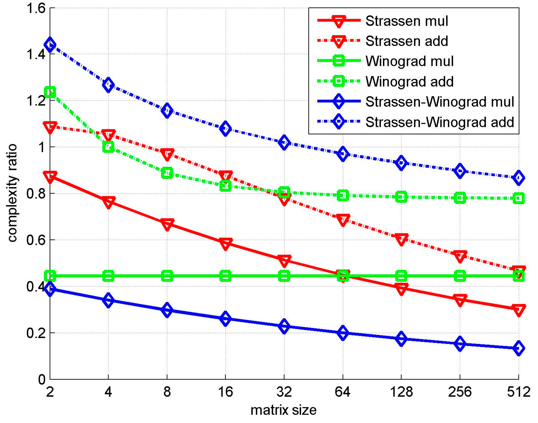
Matrix Size	Conventional		Strassen		Winograd		Strassen-Winograd
N	Mul	Add	Mul	Add	Mul	Add	Mul	Add
2	294,912	278,528	258,048	303,104	131,072	344,176	114,688	401,520
4	2,359,296	2,293,760	1,806,336	2,416,640	1,048,576	2,294,208	802,816	2,908,608
8	1.89 × 107	1.86 × 107	1.26 × 107	1.81 × 107	8.39 × 106	1.65 × 107	5.62 × 106	2.15 × 107
16	1.51 × 108	1.50 × 108	8.85 × 107	1.31 × 108	6.71 × 107	1.25 × 108	3.93 × 107	1.62 × 108
32	1.21 × 109	1.20 × 109	6.20 × 108	9.39 × 108	5.37 × 108	9.69 × 108	2.75 × 108	1.23 × 109
64	9.66 × 109	9.65 × 109	4.34 × 109	6.65 × 109	4.29 × 109	7.63 × 109	1.93 × 109	9.37 × 109
128	7.73 × 1010	7.72 × 1010	3.04 × 1010	4.68 × 1010	3.44 × 1010	6.06 × 1010	1.35 × 1010	7.19 × 1010
256	6.18 × 1011	6.18 × 1011	2.13 × 1011	3.29 × 1011	2.75 × 1011	4.83 × 1011	9.45 × 1010	5.55 × 1011
512	4.95 × 1012	4.95 × 1012	1.49 × 1012	2.31 × 1012	2.20 × 1012	3.86 × 1012	6.61 × 1011	4.29 × 1012

We can see from Table 1 that, although the algorithms cause more additions when the matrix size is small, the number of extra additions is less than the number of decreased multiplications. Moreover, multiplication usually costs more time than addition. Hence the three algorithms are all theoretically effective in reducing the computational complexity.

Figure 2 shows a comparison of the computational complexity ratios. The Strassen algorithm shows less reduction of multiplication when the matrix size is small, but it incurs less additions. The Winograd algorithm shows a stable performance. Moreover, the number of additions slightly decreases as the matrix size increases. For small-sized matrices, the Strassen-Winograd algorithm shows a much better reduction in multiplication complexity than the Strassen algorithm. Although it incurs more additions, the number of extra additions is much less than the number of decreased multiplications. The Strassen-Winograd algorithm shows a similar performance to the Winograd algorithm. When the matrix size is small, the Winograd algorithm shows a slightly better performance, whereas the Strassen-Winograd algorithm and Strassen algorithm perform much better as the matrix size increases.

Figure 2. Comparisons of the complexity ratio with different matrix sizes.

4. Simulation Results

Several simulations were conducted to evaluate our algorithm. We compare our algorithm with the Strassen algorithm and Winograd algorithm, measuring performance by the runtime in MATLAB R2013b (CPU: Inter(R) Core(TM) i7-3370K). For objectivity, we apply Equation (18) to the conventional algorithm and use it as a benchmark. Moreover, all the input data x and kernel w are randomly generated. We measure the accuracy of our algorithm by the absolute element error in the output feature maps. As a benchmark, we use the conventional algorithm with double precision data, kernels, middle variables and outputs. The other algorithms in this comparison use double precision data and kernels but single precision middle variables and outputs.

The VGG network [1] was applied to our simulation. There are nine different convolutional layers in the VGG network. The parameters of the convolutional layer are shown in Table 2. The depth indicates the number of times a layer occurs in the network. Q indicates the number of input feature maps. R indicates the number of output feature maps. Mw and Nw represent the size of the kernel. My and Ny represent the size of the output feature map. The size of the kernel in the VGG network is 3 × 3. We apply F(2 × 2, 3 × 3) to the operation of convolution. For the computation of the output feature map with size My × Ny, the map is partitioned into (My/2) × (Ny/2) sets, each using one computation of F(2 × 2, 3 × 3).

Table 2. Parameters of the convolutional layers in the Visual Geometry Group (VGG) network.

Convolutional Layer		1	2	3	4	5	6	7	8	9
Parameters	Depth	1	1	1	1	1	3	1	3	4
	Q	3	64	64	128	128	256	256	512	512
	R	64	64	128	128	256	256	512	512	512
	Mw(Nw)	3	3	3	3	3	3	3	3	3
	My(Ny)	224	224	112	112	56	56	28	28	14

As Table 2 shows, the numbers of rows and columns are not always even, and the matrices are not always square. To solve this problem, we pad a dummy row or column in the matrices once we encounter an odd number of rows or columns. The matrix can then continue using the Strassen algorithm. We apply these nine convolutional layers in turn to our simulations. For each convolutional layer, we run the four algorithms with different batch sizes from 1 to 32. The runtime consumption of the algorithms is listed in Table 3, and the numerical accuracy of the different algorithms in different layers is shown in Table 4.

Table 3. Runtime consumption of different algorithms.

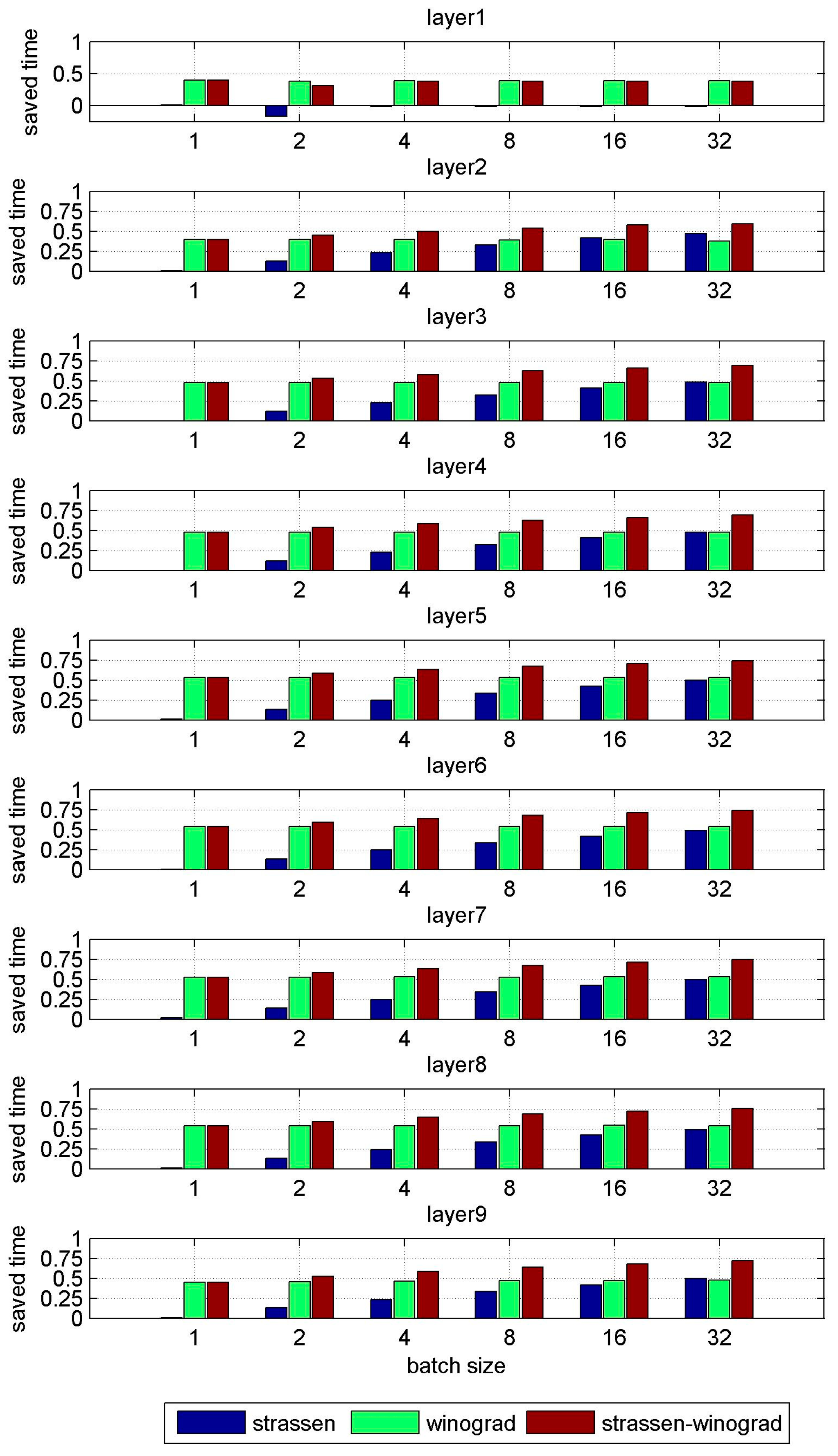
Layer	Batch Size	1	2	4	8	16	32
Layer1	Conventional	24s	48s	94s	187s	375s	752s
	Strassen	24s	56s	95s	191s	383s	768s
	Winograd	14s	29s	57s	115s	230s	462s
	Strassen-Winograd	14s	33s	58s	117s	234s	470s
Layer2	Conventional	493s	986s	1971s	3939s	7888s	15821s
	Strassen	492s	861s	1508s	2636s	4625s	8438s
	Winograd	299s	598s	1196s	2396s	4787s	9935s
	Strassen-Winograd	299s	543s	992s	1818s	3348s	6468s
Layer3	Conventional	245s	490s	980s	1962s	3916s	7858s
	Strassen	247s	433s	759s	1328s	2325s	4076s
	Winograd	128s	256s	513s	1025s	2049s	4102s
	Strassen-Winograd	128s	229s	411s	737s	1335s	2417s
Layer4	Conventional	488s	978s	1954s	3908s	7819s	15639s
	Strassen	494s	864s	1513s	2648s	4626s	8140s
	Winograd	254s	509s	1017s	2033s	4075s	8168s
	Strassen-Winograd	254s	455s	814s	1466s	2645s	4811s
Layer5	Conventional	250s	502s	1007s	2004s	4012s	8076s
	Strassen	248s	436s	761s	1328s	2317s	4078s
	Winograd	118s	236s	471s	942s	1881s	3776s
	Strassen-Winograd	118s	209s	370s	656s	1167s	2085s
Layer6	Conventional	498s	1001s	1998s	3995s	7948s	15892s
	Strassen	494s	868s	1507s	2646s	4643s	8102s
	Winograd	231s	462s	923s	1844s	3693s	7382s
	Strassen-Winograd	231s	410s	725s	1286s	2296s	4089s
Layer7	Conventional	244s	487s	980s	1940s	3910s	7820s
	Strassen	241s	421s	739s	1283s	2250s	3961s
	Winograd	116s	231s	461s	920s	1839s	3680s
	Strassen-Winograd	116s	204s	358s	630s	1111s	1961s
Layer8	Conventional	479s	955s	1917s	3833s	7675s	15319s
	Strassen	474s	829s	1453s	2546s	4447s	7811s
	Winograd	222s	443s	884s	1766s	3524s	7068s
	Strassen-Winograd	223s	391s	686s	1210s	2129s	3772s
Layer9	Conventional	118s	237s	474s	951s	1900s	3823s
	Strassen	117s	206s	362s	631s	1107s	1937s
	Winograd	65s	128s	254s	507s	1009s	2010s
	Strassen-Winograd	65s	113s	197s	345s	606s	1063s

Table 4. Maximum element error of different algorithms in different layers.

	Conventional	Strassen	Winograd	Strassen-Winograd
Layer1	1.25 × 10−6	3.03 × 10−6	2.68 × 10−6	4.01 × 10−6
Layer2	2.46 × 10−5	7.59 × 10−5	4.62 × 10−5	9.50 × 10−5
Layer3	2.65 × 10−5	7.23 × 10−5	4.83 × 10−5	9.51 × 10−5
Layer4	4.94 × 10−5	1.50 × 10−4	9.40 × 10−5	1.78 × 10−4
Layer5	5.14 × 10−5	1.46 × 10−4	1.00 × 10−4	1.74 × 10−4
Layer6	9.80 × 10−5	2.94 × 10−4	1.88 × 10−4	3.50 × 10−4
Layer7	9.92 × 10−5	2.82 × 10−4	1.79 × 10−4	3.39 × 10−4
Layer8	2.09 × 10−4	5.89 × 10−4	3.51 × 10−4	6.99 × 10−4
Layer9	1.84 × 10−4	5.76 × 10−4	3.50 × 10−4	6.16 × 10−4

Table 4 shows that the Winograd algorithm is slightly more accurate than the Strassen algorithm and Strassen-Winograd algorithm. The maximum element error of these algorithms is 6.16 × 10⁻⁴. Compared with the minimum value of 1.09 × 10³ in the output feature map, the accuracy loss incurred by these algorithms is negligible. As we can see from Section 2, theoretically, the processes in all of these algorithms do not result in a loss in accuracy. In practice, a loss in accuracy is mainly caused by the single precision data. Because the conventional algorithm with low precision data is sufficiently accurate for deep learning [10,11], we conclude that the accuracy of our algorithm is equally sufficient.

To compare runtime easily, we use the conventional algorithm as a benchmark, and calculate the saving on runtime displayed by the other algorithms. The result is shown in Figure 3.

Figure 3. Comparisons with different batch sizes.

The Strassen-Winograd algorithm shows a better performance than the benchmark in all layers except layer1. This is because the number of input feature maps Q in layer1 is three, which limits the performance of the algorithm as a small matrix size incurs more additions. Moreover, odd numbers of rows or columns need dummy rows or columns for matrix partitioning, which causes more runtime.

The performance of the Winograd algorithm is stable from layer2 to layer9. It saves 53% of the runtime on average, which is close to the 56% reduction in multiplications. The performances of the Strassen algorithm and Strassen-Winograd algorithm improve as the batch size increases. For example, in layer7, when the batch size is 1, we cannot partition the matrix to use the Strassen algorithm, and there is almost no saving on runtime. The Strassen-Winograd algorithm saves 52% of the runtime, a similar saving as the Winograd algorithm. When the batch size is 2, the Strassen algorithm saves 13% of the runtime, which equates to the 13% reduction in multiplications. The Strassen-Winograd algorithm saves 58% of the runtime, which is close to the 61% reduction in multiplications. As the batch size increases, the Strassen algorithm and Strassen-Winograd algorithm can use more recursions, which can further reduce the number of multiplications and save more runtime. When the batch size is 32, the Strassen-Winograd algorithm saves 75% of the runtime, while the Strassen algorithm and Winograd algorithm save 49% and 53%, respectively.

Though experiments with larger batch sizes were not carried out due to limitations on time and memory, we can see the trend in performance as the batch size increases. This is consistent with the theoretical analysis in Section 3. We conclude therefore that the proposed algorithm can provide the optimal performance by combining the savings of these two algorithms.

5. Conclusions and Future Work

The computational complexity of convolutional neural networks is an urgent problem for real-time applications. Both the Strassen algorithm and Winograd algorithm are effective in reducing the computational complexity without losing accuracy. This paper proposed to combine these algorithms to reduce the heavy computational burden. The proposed strategy was evaluated with the VGG network. Both the theoretical performance assessment and the experimental results show that the Strassen-Winograd algorithm can dramatically reduce the computational complexity.

There remain limitations that need to be addressed in future research. Although the algorithm reduces the computational complexity of convolutional neural networks, the cost is an increased difficulty in implementation, especially in real-time systems and embedded devices. It also increases the difficulty of parallelizing an artificial network for hardware acceleration. In future work, we aim to apply this method to hardware accelerator using practical applications.

References

- Simonyan, K.; Zisserman, A. Very deep convolutional networks for large-scale image recognition. arXiv, 2014; arXiv:1409.1556. [Google Scholar]
- Liu, N.; Wan, L.; Zhang, Y.; Zhou, T.; Huo, H.; Fang, T. Exploiting Convolutional Neural Networks with Deeply Local Description for Remote Sensing Image Classification. IEEE Access 2018, 6, 11215–11228. [Google Scholar] [CrossRef]
- Krizhevsky, A.; Sutskever, I.; Hinton, G.E. ImageNet classification with deep convolutional neural networks. In Proceedings of the International Conference on Neural Information Processing Systems, 3–6 December 2012; Volume 60, pp. 1097–1105. [Google Scholar]
- Le, N.M.; Granger, E.; Kiran, M. A comparison of CNN-based face and head detectors for real-time video surveillance applications. In Proceedings of the Seventh International Conference on Image Processing Theory, Tools and Applications, Montreal, QC, Canada, 28 November–1 December 2018. [Google Scholar]
- Ren, S.; He, K.; Girshick, R. Faster R-CNN: Towards real-time object detection with region proposal networks. In Proceedings of the International Conference on Neural Information Processing Systems, Montreal, QC, Canada, 8–13 December 2014; pp. 91–99. [Google Scholar]
- Denil, M.; Shakibi, B.; Dinh, L. Predicting Parameters in Deep Learning. In Proceedings of the International Conference on Neural Information Processing Systems, Lake Tahoe, NV, USA, 5–10 December 2013; pp. 2148–2156. [Google Scholar]
- Han, S.; Pool, J.; Tran, J. Learning both Weights and Connections for Efficient Neural Networks. In Proceedings of the International Conference on Neural Information Processing Systems, Istanbul, Turkey, 9–12 November 2015; pp. 1135–1143. [Google Scholar]
- Guo, Y.; Yao, A.; Chen, Y. Dynamic Network Surgery for Efficient DNNs. In Advances in Neural Information Processing Systems; MIT Press: Cambridge, MA, USA, 2016; pp. 1379–1387. [Google Scholar]
- Qiu, J.; Wang, J.; Yao, S. Going Deeper with Embedded FPGA Platform for Convolutional Neural Network. In Proceedings of the ACM/SIGDA International Symposium on Field-Programmable Gate Arrays, Monterey, CA, USA, 21–23 February 2016; pp. 26–35. [Google Scholar]
- Courbariaux, M.; Bengio, Y.; David, J.P. Low Precision Arithmetic for Deep Learning. arXiv, 2014; arXiv:1412.0724. [Google Scholar]
- Gupta, S.; Agrawal, A.; Gopalakrishnan, K.; Narayanan, P. Deep Learning with Limited Numerical Precision. In Proceedings of the International Conference on Machine Learning, Lille, France, 7–9 July 2015. [Google Scholar]
- Rastegari, M.; Ordonez, V.; Redmon, J. XNOR-Net: ImageNet Classification Using Binary Convolutional Neural Networks. In Proceedings of the European Conference on Computer Vision, Amsterdam, The Netherlands, 11–14 October 2016; Springer: Cham, Switzerland, 2016; pp. 525–542. [Google Scholar]
- Zhu, C.; Han, S.; Mao, H. Trained Ternary Quantization. In Proceedings of the International Conference on Learning Representations, Toulon, France, 24–26 April 2017. [Google Scholar]
- Zhang, X.; Zou, J.; Ming, X.; Sun, J. Efficient and accurate approximations of nonlinear convolutional networks. In Proceedings of the Computer Vision and Pattern Recognition, Boston, MA, USA, 7–12 June 2014; pp. 1984–1992. [Google Scholar]
- Mathieu, M.; Henaff, M.; Lecun, Y.; Chintala, S.; Piantino, S.; Lecun, Y. Fast Training of Convolutional Networks through FFTs. arXiv, 2013; arXiv:1312.5851. [Google Scholar]
- Vasilache, N.; Johnson, J.; Mathieu, M. Fast Convolutional Nets with fbfft: A GPU Performance Evaluation. In Proceedings of the International Conference on Learning Representations, San Diego, CA, USA, 7–9 May 2015. [Google Scholar]
- Toom, A.L. The complexity of a scheme of functional elements simulating the multiplication of integers. Dokl. Akad. Nauk SSSR 1963, 150, 496–498. [Google Scholar]
- Cook, S.A. On the Minimum Computation Time for Multiplication. Ph.D. Thesis, Harvard University, Cambridge, MA, USA, 1966. [Google Scholar]
- Winograd, S. Arithmetic Complexity of Computations; SIAM: Philadelphia, PA, USA, 1980. [Google Scholar]
- Jiao, Y.; Zhang, Y.; Wang, Y.; Wang, B.; Jin, J.; Wang, X. A novel multilayer correlation maximization model for improving CCA-based frequency recognition in SSVEP brain-computer interface. Int. J. Neural Syst. 2018, 28, 1750039. [Google Scholar] [CrossRef] [PubMed]
- Wang, R.; Zhang, Y.; Zhang, L. An adaptive neural network approach for operator functional state prediction using psychophysiological data. Integr. Comput. Aided Eng. 2015, 23, 81–97. [Google Scholar] [CrossRef]
- Lavin, A.; Gray, S. Fast Algorithms for Convolutional Neural Networks. In Proceedings of the Computer Vision and Pattern Recognition, Caesars Palace, NV, USA, 26 June–1 July 2016; pp. 4013–4021. [Google Scholar]
- Strassen, V. Gaussian elimination is not optimal. Numer. Math. 1969, 13, 354–356. [Google Scholar] [CrossRef]
- Cong, J.; Xiao, B. Minimizing Computation in Convolutional Neural Networks. In Proceedings of the Artificial Neural Networks and Machine Learning—ICANN 2014, Hamburg, Germany, 15–19 September 2014. [Google Scholar]