Article

Online Uniformly Inserting Points on the Sphere †

1
Research Center for High Performance Computing, Joint Engineering Research Center for Health Big Data Intelligent Analysis Technology, Shenzhen Institutes of Advanced Technology, Chinese Academy of Sciences, 1068 Xueyuan Avenue, Shenzhen University Town, Shenzhen 518055, China
2
University of Chinese Academy of Sciences, 19(A) Yuquan Road, Shijingshan District, Beijing 100049, China
3
Department of Computer Science, The University of Hong Kong, Pokfulam, Hong Kong, China
4
School of Computer Science, University of Nottingham Ningbo China, 199 Taikang East Road, Ningbo 315100, China
*
Author to whom correspondence should be addressed.
This paper is an extended version of our paper published in the 11th International Conference and Workshops on Algorithms and Computation (WALCOM 2017).
Algorithms 2018, 11(10), 156; https://doi.org/10.3390/a11100156
Submission received: 11 August 2018 / Revised: 25 September 2018 / Accepted: 11 October 2018 / Published: 16 October 2018

Abstract

:
Uniformly inserting points on the sphere has been found useful in many scientific and engineering fields. Different from the offline version where the number of points is known in advance, we consider the online version of this problem. The requests for point insertion arrive one by one and the target is to insert points as uniformly as possible. To measure the uniformity we use gap ratio which is defined as the ratio of the maximal gap to the minimal gap of two arbitrary inserted points. We propose a two-phase online insertion strategy with gap ratio of at most 3.69 . Moreover, the lower bound of the gap ratio is proved to be at least 1.78 .

1. Introduction

Uniformly distributing points over a specific domain has many applications in digital halftoning, numerical integration, computer graphics, etc. For the offline version, the number of points is known in advance, which is to configure N points as evenly as possible on a metric space, and attention is paid to the final uniformity of this N-point configuration rather than the uniformity in the process. Different from the offline version, the online version of this problem considers the situation of point insertion requests arriving one by one. Because the total number of points is unknown, points are required to be inserted as uniformly as possible in each insertion step.
According to known online algorithms, there are several ways to estimate the uniformity of the distribution of the points. To measure the uniformity of points, there are several metrics. Some studies use the minimum pairwise distance [1,2] to measure the uniformity. Some other studies take the uniformity problem as minimal energy problems [3]. In discrepancy theory [4,5], uniformity can be defined by the spherical cap discrepancy, which is the supremum of the local discrepancy over all spherical caps. Ref. [6] showed that the spherical cap discrepancy of random point sets, of spherical digital nets and of spherical Fibonacci lattices converges with order N 1 / 2 . Ref. [7] established connections to spherical cap discrepancy and showed some general discrepancy bounds. Uniformity can also be defined by the ratio between the maximal and minimal number of points in a fixed shape within the area.

1.1. Related Works

For the case of uniformly inserting points in a 2-dimensional plane, Teramoto et al. [8] and Asano et al. [9] proposed a greedy algorithm using the Voronoi insertion strategy, which works well and the gap ratio is proved to be at most 2. They also studied insertion onto a 1-dimensional line. If the number n of the points is known in advance, an insertion strategy with the gap ratio 2 n / 2 / ( n / 2 + 1 ) can be achieved. If the points can only be inserted at the fixed grid, Asano [10] gave an insertion strategy with uniformity 2 for 1-dimensional case. For the case of uniformly inserting points into a square, Zhang et al. [11] proved the lower bound to be at least 2.5 and gave an insertion algorithm with the maximal gap ratio 2.828. Recently, Bishnu et al. [12] attempted to generalize an approximation algorithm framework over all metric spaces. It generates different gap ratios for different metric spaces and the lower bounds for several specific metric spaces are calculated.

1.2. Our Contribution

We consider a special case of the point insertion problem, that is, how to insert points on a sphere as uniformly as possible. To solve the above problem, we proposed an insertion algorithm based on a regular dodecahedron with gap ratio no more than 5.99 in our previous work [13]. In this paper, by a more detailed analysis on specific cases, the upper bound of the maximal gap ratio is improved to 3.69 . Moreover, the lower bound of the maximal gap ratio is proved to be at least 1.78 .

2. Materials and Methods

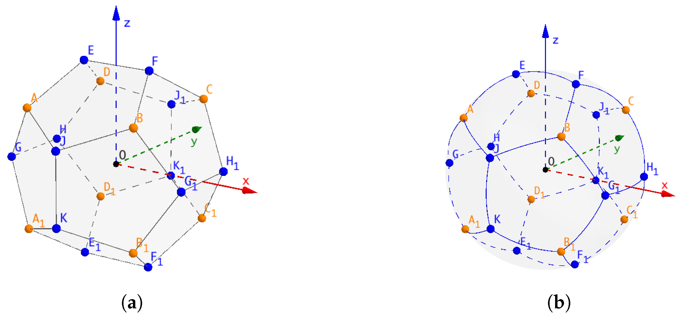
2.1. Problem Description

The problem of inserting points on a sphere dates back to J.J. Thomson in 1904 [14]. It aimed to find a configuration of n electrons on a sphere so as to minimize the electrostatic potential energy. It played an important role in many scientific and engineering applications [15,16,17], such as 3D projection reconstruction of Computed Tomography (CT) or Magnetic Resonance Images (MRI).
Formally speaking, there is a point sequence { p 1 , p 2 , , p i , } to be inserted on a sphere S. When inserting the i-th point, p i denotes its position and S i = p 1 , , p i denotes the configuration after inserting this point. In configuration S i , define the maximal gap to be
G i = max p S min q S i 2 d ( p , q )
and the minimal gap to be
g i = min p , q S i , p q d ( p , q )
where d ( p , q ) is the spherical distance between p and q. Note that G i can also be regarded as the length of arc corresponding to the maximal empty spherical area.
The gap ratio is defined as
r i = G i g i = max p S min q S i 2 d ( p , q ) min p , q S i , p q d ( p , q )
The objective is to minimize the maximal gap ratio ( min max i r i ) for each insertion.

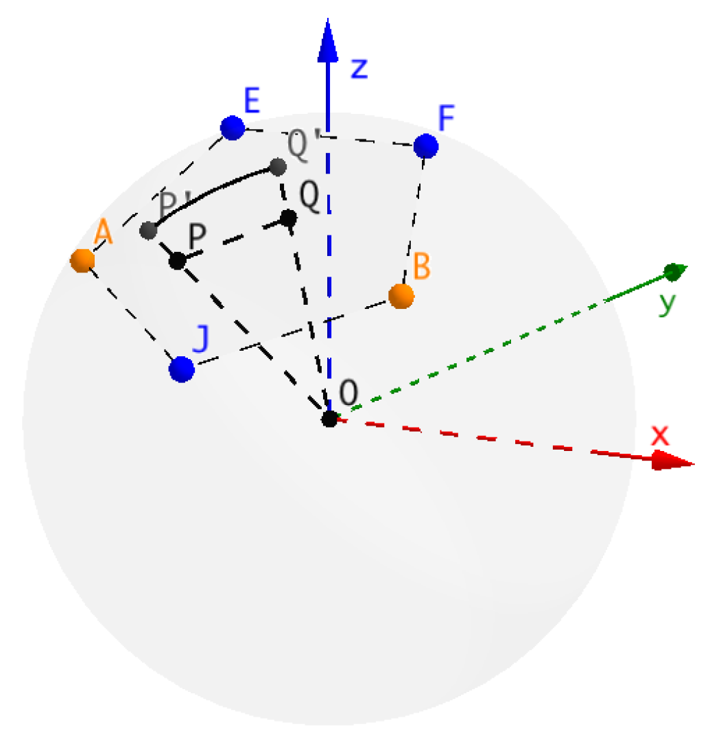
2.2. The Insertion Strategy

A simple intuitive idea is to greedily insert the incoming point at the “center” of the largest empty spherical surface area. The early steps of such a greedy approach are simple; however, when many points have been inserted, the shapes of different local structures may vary significantly and the configuration may become very complicated. As a result, the computational cost of finding the largest empty spherical surface area and then computing its center may become prohibitive. Observe that once some points have been inserted, the sphere is partitioned into local structures and the next point insertion within the area of some local structure will only affect the local configuration there, i.e., the spherical distances (including the max gap and min gap) outside this area do not change. Based on this observation, a two-phase strategy can be devised.
Let us consider a regular dodecahedron instead of the sphere. A regular dodecahedron has 12 identical regular pentagonal faces and 20 vertices, as shown in Figure 1a. For the convenience of computation, we can assume that the radius of the sphere is 3 and thus the length of each edge of the corresponding regular dodecahedron is 4 / ( 5 + 1 ) .
In the first phase, handling the insertion of 20 points on the sphere is quite straightforward: First insert eight orange points at vertices with coordinates ( ± 1 , ± 1 , ± 1 ) . Two arbitrary opposite vertices, for example, A, C 1 , of the orange cube are inserted first, followed by the remaining 6 points in any arbitrary order. Then insert the remaining 12 points in any arbitrary order, as 6 structures of the same shape for every 2 points on the plane of the cube. The maximal gap ratio in this phase is proved to be 2.618 [13].
In the second phase, since the projection of the regular dodecahedron’s edges divides the sphere into 12 identical curved surface areas, as shown in Figure 1b, we can consider point insertion in each local structure.
In the previous work [13], we proved that for any two points ( P , Q ) inside a pentagon (for example, as shown in Figure 2, ( P , Q ) P e n t a g o n A J B F E , with ( P , Q ) denoting their projection on the sphere), the gap ratio on the plane (pentagon) is smaller than that on the sphere, and we proved the difference can be reduced to 1.34 [13]. Therefore, the comparison between two spherical distances can be reduced to the comparison between two direct distances and the ratio would not change much.
We also proposed an insertion strategy in a pentagon in the previous work [13] as shown in Figure 3a, each pentagon can be partitioned into 1 smaller pentagon and 5 acute isosceles triangles with vertex angle of π 5 . An acute isosceles triangle can be further partitioned into 1 smaller acute isosceles triangle with vertex angle of π 5 , as shown in Figure 3b and 1 obtuse isosceles triangle with vertex angle of 3 π 5 , as shown in Figure 3c. An obtuse isosceles triangle can be partitioned into 1 acute isosceles triangle and 2 obtuse isosceles triangles. In this way, the pentagon is recursively partitioned into 3 types of shapes, which will be stored in 3 queues respectively.
When a new point comes in, we first compare the insertions on the heads of these three queues and select the one with the largest minimal gap r if the point is inserted at an appropriate position. The incoming point is inserted on the corresponding shape, and the head of the queue is removed, and smaller shapes generated after point insertion are added to the tail of the corresponding queues. Finally, the projected position on the sphere of the inserted point is calculated.

3. Results

By analyzing point insertions step by step, the upper bound of the gap ratio is proved to be at most 3.69 . Moreover, the lower bound of the gap ratio is proved to be at least 1.78 . Below is the detailed description.

3.1. Analysis of the Upper Bound

We prove that the maximal gap ratio in the first phase is 2.618 , and the maximal gap ratio in the second phase is 5.99 . However, by analyzing point insertions in a pentagon step by step, the upper bound can be improved to 3.69 .

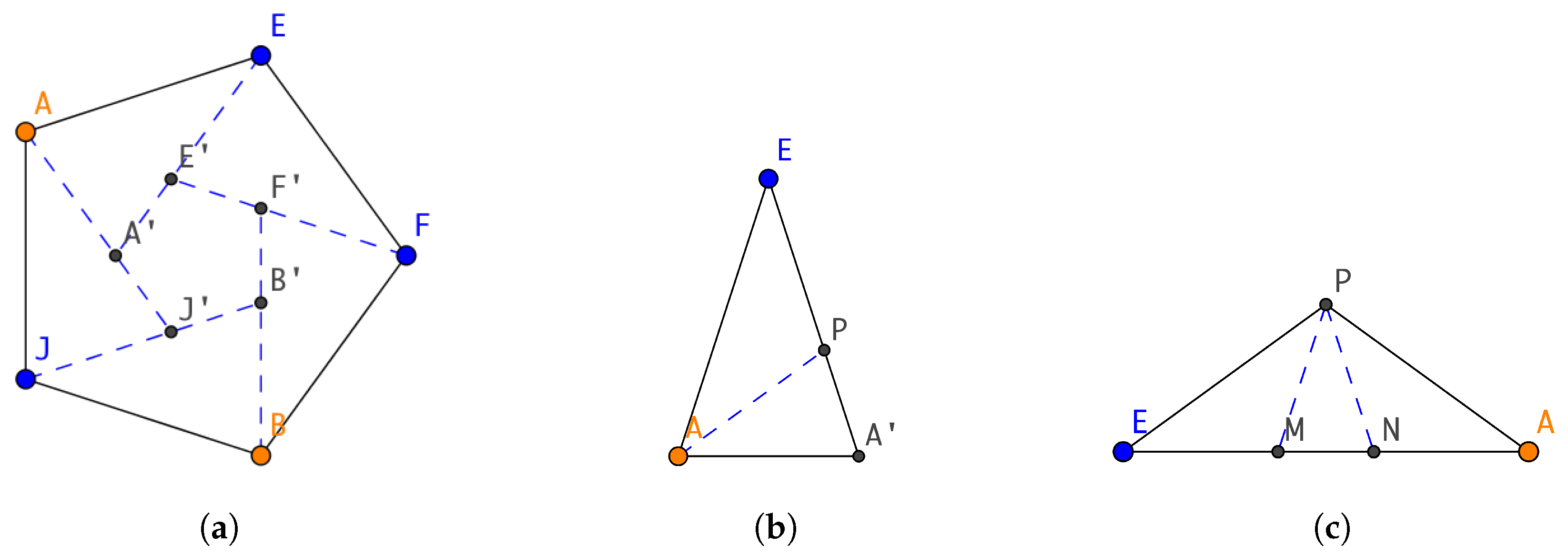
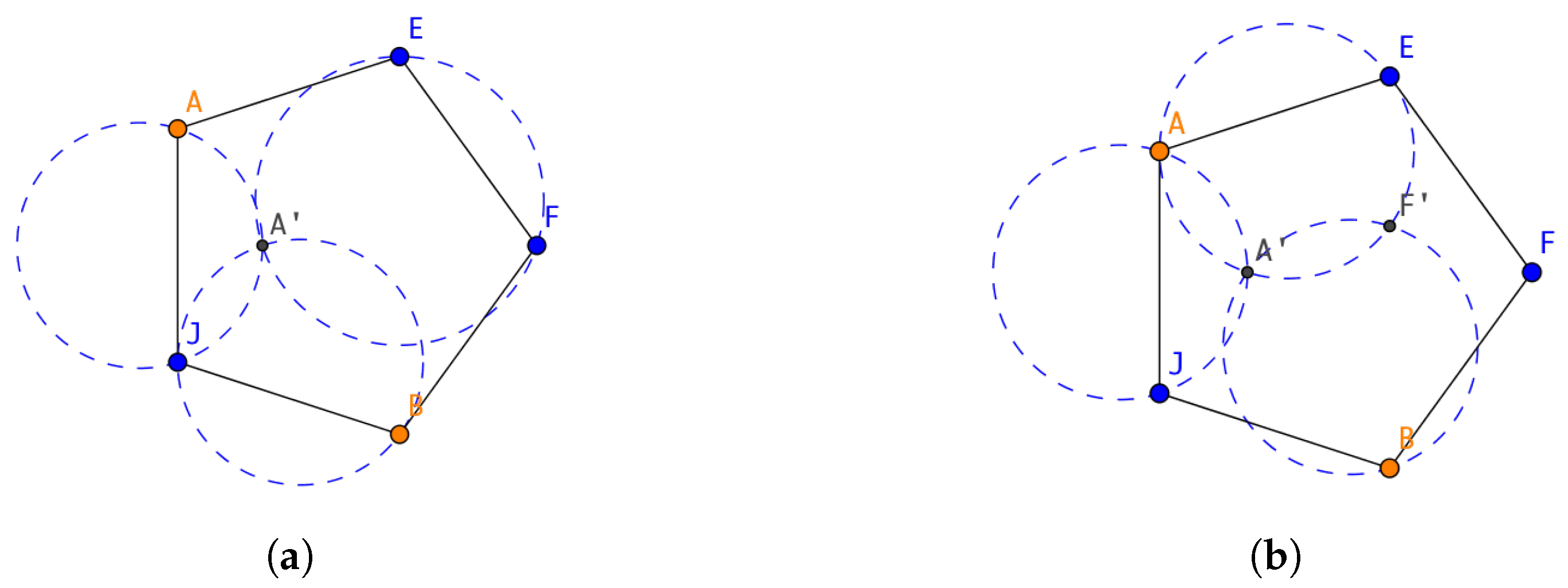
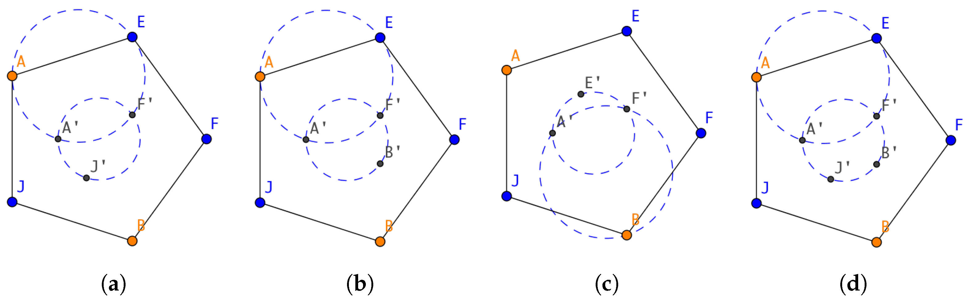
3.1.1. Inserting Points in a Pentagon

For point insertions in each pentagon, there are 5 positions for consideration. Here we compute the gap ratio step by step.
Consider the pentagon A J B F E in Figure 3a, assuming that the edge of pentagon A J B F E is l, and w.l.o.g., point A is inserted first. According to the definition, the maximal gap is the diameter of the circumcircle of Δ A E F , as shown in Figure 4a. By the law of sines, we have G A = | A E | sin A F E = l sin ( π 2 π 5 ) / 2 = 1.236 l , and the minimal gap is g A = | A A | = 2 l 2 ( 1 cos π 5 ) = 0.618 l . Therefore, the gap ratio after the first point insertion on the pentagon is r A = 1.34 · G A g A = 2.68 .
For the second point F on the pentagon, as shown in Figure 4b, the maximal gap is the diameter of the circumcircle of Δ A B F , G F = | A B | sin A F B = l sin 2 π 5 = 1.051 l , and the minimum gap is g F = | A F | = | A A | = 0.618 l . Thus, the gap ratio after the second point insertion on the pentagon is r F = 1.34 · G F g F = 2.28 .
After the insertion of the two points A , F , the insertion order will not affect the gap ratio. For the third point and the fourth point, see Figure 5, the maximal gap will be the diameter of the circumcircle of quadrangle A A F E or the circumcircle of Δ A F B , which is equal to 1.051 l , and the minimal gap equals to the edge of the internal pentagon A J B F E , which is 0.382 l . So the gap ratio after the third and forth point insertion on the pentagon is r 3 , 4 = 1.34 · G g = 3.69 .
For the fifth point, the maximal gap will be the diameter of the circumcircle of pentagon A J B F E , which is equal to 0.382 l sin π 5 = 0.650 l , and the minimal gap equals to the edge of pentagon A J B F E , which is 0.382 l . So the gap ratio after the fifth point insertion on the pentagon is r 5 = 1.34 · G g = 2.28 .
Therefore, the gap ratio for points insertion inside the pentagon r 3.69 .

3.1.2. Inserting Points in an Acute Isosceles Triangle

As shown in Figure 3b, the maximal gap equals the diameter of the circumcircle of Δ A P A , i.e., G P = | A A | sin 2 π 5 = 1.051 | A A | , and the minimal gap is | P A | , i.e., g P = 2 | A A | 2 ( 1 cos π 5 ) = 0.618 | A A | . So the gap ratio is at most r P = 1.34 · G P g P = 2.28 .

3.1.3. Inserting Points in an Obtuse Isosceles Triangle

For the point insertion in an obtuse isosceles triangle, the computation is similar to the previous case.
For the first point insertion, for example, inserting N, the maximal gap is the diameter of circumcircle of Δ P E N , i.e., G N = | P E | sin π 5 = 1.051 | P E | . The minimal gap is | P N | , i.e., g N = | P N | = 2 | P E | 2 ( 1 cos π 5 ) = 0.618 | P E | . The gap ratio at this stage is r N = 1.34 · G N g N = 2.28 .
For the second point insertion, after inserting M, the maximal gap is the diameter of the circumcircle of Δ P M N , i.e., G M = | M N | sin π 5 = 1.701 | M N | . The minimal gap is | M N | , i.e., g M = | M N | . The gap ratio at this stage is r M = 1.34 · G M g M = 2.28 .
Thus, the gap ratio of inserting points in an obtuse isosceles triangle is at most 2.28 .
Combining all the above cases, we have the following concluding theorem.
Theorem 1.
The maximal gap ratio of the insertion strategy is at most 3.69 .

3.2. Analysis of the Lower Bound

We estimate lower bound for inserting a point sequence on the sphere of P = ( p 1 , p 2 , , p i , ) on the sphere. In this section, we compare the gap ratio after each point insertion and pick out the minimal one, which can be described as: r l b = inf max { r 1 , r 2 , , r i , } .

3.2.1. 2-Point Sequence Insertion

For the 2-point sequence case, the first point is placed arbitrarily, and then the second point should be on the same orthodrome. Let the central angle between p 1 and p 2 be α , as shown in Figure 6a, and the gap ratio is
r 2 = G 2 g 2 = 2 π α α
Obviously, the minimal gap ratio is 1 when α = π .

3.2.2. 3-Point Sequence Insertion

Lemma 1.
For 3-point sequence insertions, the gap ratio is no less than 1.78 .
Proof of Lemma 1.
Insert points p 1 , p 2 , p 3 one after another. After inserting p 1 and p 2 , we have Equation (4) according to the previous case.
After inserting point p 3 , these 3 points determine a plane which intersects the sphere. Let R denote the radius of the sphere, O denote the center of the circumcircle of Δ p 1 p 2 p 3 , and r denote the radius of the circumcircle; and let p 1 O p 2 = β , p 2 O p 3 = γ , O O p 1 = δ . Obviously, G 3 = 2 R ( π δ ) . W.l.o.g., assuming that 0 < γ 2 π β γ β < π and 0 < δ π / 2 , we have g 3 = d ( p 2 , p 3 ) = R · p 2 O p 3 . Thus,
r 3 = G 3 g 3 = 2 ( π δ ) p 2 O p 3
By the law of cosines, we have | p 2 p 3 | 2 = 2 R 2 ( 1 cos p 2 O p 3 ) for Δ O p 2 p 3 , and we also have | p 2 p 3 | 2 = 2 r 2 ( 1 cos γ ) for Δ O p 2 p 3 , where r is the radius of the circumcircle of Δ p 1 p 2 p 3 , and r = R sin δ . Combining these two equations we have p 2 O p 3 = arccos ( 1 sin 2 δ ( 1 cos γ ) ) .
In the same way, we can get the value of α , α = p 1 O p 2 = arccos ( 1 sin 2 δ ( 1 cos β ) ) .
So we have
r 2 = 2 π arccos ( 1 sin 2 δ ( 1 cos β ) ) arccos ( 1 sin 2 δ ( 1 cos β ) )
r 3 = 2 ( π δ ) arccos ( 1 sin 2 δ ( 1 cos γ ) )
In order to get to lower bound, we should find the minimum gap ratio for the worst case of { r 2 , r 3 } . In this way, the lower bound must exist in the case where r 2 = r 3 . As δ is independent to other parameters, we first compute the partial derivative to δ : d r 3 d δ = sin 2 δ ( 1 cos β ) arccos 2 χ 1 χ 2 < 0 , where χ = 1 sin 2 δ ( 1 cos β ) . In the same way, d r 2 d δ < 0 . So the gap ratio of r 3 and r 2 is a decrement function w.r.t. δ . Thus, the minimal gap is achieved when δ = π / 2 where all the three points are on the spherical large arc.
So we set δ = π / 2 and let r 2 = r 3 , and we get γ = π β 2 π β . By the assumption that 0 < γ 2 π β γ β < π , we can finally get:
γ = π β 2 π β γ 2 π β 2 γ 2 ( π β )
By solving (6), we can get 0.719 π β 0.764 π . Considering that with δ fixed, the gap ratio is a decreasing function w.r.t. β . In this case, the minimal gap ratio is 1.78 . ☐

3.2.3. More Point Sequence Insertion

Lemma 2.
For more than three points, the gap ratio is no less than 1.78 .
Proof of Lemma 2.
In each step of the online insertion, we compute the gap ratio and hope it to be the lowest. After inserting the first three points, the gap ratio can be expressed as r = d e s a d m i n , where d e s a is the arc corresponding to the maximal empty spherical area, and d m i n is the minimum arc. We use sequence δ 3 , δ 4 , , δ n 1 , δ n to denote the center angle for the largest spherical area and sequence d 3 , d 4 , , d n 1 , d n to denote the distance for the minimum arc at each step.
Similarly, the minimum gap ratio will exist on the condition that r 2 = r 3 = r 4 = = r n 1 = r n , which is equal to R δ 3 d 3 = R δ 4 d 4 = = R δ n 1 d n 1 = R δ n d n . Since we insert the point in order to ensure the gap ratio is the lowest in each step, we have δ 3 = δ 4 . Moreover, as 0 d n d n 1 d 3 , we have 0 γ n γ n 1 γ 4 ( π γ 4 ) . Thus, we have γ 3 π / 2 . Since r 3 is a decreasing function about γ 3 , the minimum gap ratio will not be less than 1.78 regardless of the values of α and β . ☐
Theorem 2.
The minimal gap ratio of inserting points on the sphere is no less than 1.78 .

3.3. Analysis of Computational Complexity

In the first phase of the proposed algorithm, 20 vertices are inserted and a queue of 12 regular pentagons are added to the pentagon-queue. In the second phase, the algorithm focuses on 3 local structures: Pentagons, acute triangles, and obtuse triangles. When a new point arrives, we first determine which queue the new point is to be added to:
  • If the pentagon queue is selected, insertion of 5 points will lead to removing the head of the queue. Meanwhile, a smaller pentagon and five smaller acute triangles will be added to the tail of the corresponding queues respectively.
  • If the acute triangle queue is selected, insertion of 1 point will lead to removing the head of the queue. Meanwhile, a smaller acute triangle and a smaller obtuse triangle will be added to the tail of the corresponding queues respectively.
  • If the obtuse triangle queue is selected, insertion of 2 points will lead to removing the head of the queue. Meanwhile, a smaller acute triangle and 2 smaller obtuse triangles will be added to the tail of the corresponding queues respectively.
For each point insertion, the comparison and growth of the queues, and the projection calculation of inserted point onto the sphere are constant, and so the computational cost is O ( 1 ) . After n points have been inserted, the computational complexity is O ( n ) .

4. Discussion

Is it possible to further reduce the gap ratio by using other structures? How about some simpler regular structures, e.g., isocahedron? If we split the isocahedron into four congruent sub-triangles regularly, the gap ratio will be larger since the newly inserted points are on the side of the isocahedron. From the definition, the maximal gap is the spherical diameter of the largest empty circle while the minimal gap is the minimal spherical distance between two inserted points. So, if points are inserted on the side of some configuration, the ratio is not going to be good.

5. Conclusions

Uniform insertion of points is an interesting problem in computer science. In this paper, we use the gap ratio to measure the uniformity of online insertion. We first give a two-phase online insertion strategy with the help of the regular dodecahedron, and then prove that the gap ratio is at most 3.69 and at least 1.78 .

Author Contributions

Conceptualization, S.-H.P. and Y.Z.; Methodology, R.Z., C.C.and Y.Z.; Formal Analysis, R.Z. and C.C.; Writing—Original Draft Preparation, R.Z. and C.C.; Writing—Review & Editing, F.C.M.L. and Y.Z.; Visualization, R.Z.; Supervision, F.C.M.L. and Y.Z.; Funding Acquisition, L.S., F.C.M.L. and Y.Z.

Funding

This research is supported by China’s NSFC grants (No. 61433012, U1435215), Hong Kong GRF grant (17210017), and Shenzhen research grant JCYJ20160229195940462 and GGFW2017073114031767.

Conflicts of Interest

The authors declare no conflict of interest.

References

  1. Nurmela, K.J.; Ostergard, P.R.J. More Optimal Packings of Equal Circles in a Square. Discret. Comput. Geom. 1999, 22, 439–457. [Google Scholar] [CrossRef]
  2. Collins, C.R.; Stephenson, K. A circle packing algorithm. Comput. Geom. Theory Appl. 2003, 25, 233–256. [Google Scholar] [CrossRef]
  3. García, A.; Saff, E. Asymptotics of greedy energy points. Math. Comput. 2010, 79, 2287–2316. [Google Scholar] [CrossRef]
  4. Matousek, J. Geometric Discrepancy: An Illustrated Guide; Springer: Berlin/Heidelberg, Germany, 1999. [Google Scholar]
  5. Chazelle, B. The Discrepancy Method: Randomness and Complexity; Cambridge University Press: New York, NY, USA, 2000. [Google Scholar]
  6. Aistleitner, C.; Brauchart, J.S.; Dick, J. Point sets on the sphere 𝕊2 with small spherical cap discrepancy. Discret. Comput. Geom. 2012, 48, 990–1024. [Google Scholar]
  7. Grabner, P.J.; Tichy, R.F. Spherical designs, discrepancy and numerical integration. Math. Comput. 1993, 60, 327–336. [Google Scholar] [CrossRef]
  8. Teramoto, S.; Asano, T.; Katoh, N.; Doerr, B. Inserting points uniformly at every instance. IEICE Trans. Inf. Syst. 2006, 89, 2348–2356. [Google Scholar] [CrossRef]
  9. Asano, T.; Teramoto, S. On-line uniformity of points. In Proceedings of the Book of Abstracts for 8th Hellenic-European Conference on Computer Mathematics and its Applications, Athens, Greece, 8–11 July 2007; pp. 21–22. [Google Scholar]
  10. Asano, T. Online uniformity of integer points on a line. Inf. Proc. Lett. 2008. [Google Scholar] [CrossRef]
  11. Zhang, Y.; Chang, Z.; Chin, F.Y.; Ting, H.F.; Tsin, Y.H. Uniformly inserting points on square grid. Inf. Proc. Lett. 2011, 111, 773–779. [Google Scholar] [CrossRef]
  12. Bishnu, A.; Desai, S.; Ghosh, A.; Goswami, M.; Paul, S. Uniformity of point samples in metric spaces using gap ratio. SIAM J. Discret. Math. 2017, 31, 2138–2171. [Google Scholar] [CrossRef]
  13. Chen, C.; Lau, F.C.; Poon, S.H.; Zhang, Y.; Zhou, R. Online Inserting Points Uniformly on the Sphere. In Proceedings of the International Workshop on Algorithms and Computation, Hsinchu, Taiwan, 29–31 March 2017; pp. 243–253. [Google Scholar]
  14. Thomson, J.J. On the structure of the atom: An investigation of the stability and periods of oscillation of a number of corpuscles arranged at equal intervals around the circumference of a circle; with application of the results to the theory of atomic structure. Lond. Edinb. Dublin Philos. Mag. J. Sci. 1904, 7, 237–265. [Google Scholar] [CrossRef]
  15. Hicks, J.S.; Wheeling, R.F. An efficient method for generating uniformly distributed points on the surface of an n-dimensional sphere. Commun. ACM 1959, 2, 17–19. [Google Scholar] [CrossRef]
  16. Koay, C.G. Analytically exact spiral scheme for generating uniformly distributed points on the unit sphere. J. Comput. Sci. 2011, 2, 88–91. [Google Scholar] [CrossRef] [PubMed] [Green Version]
  17. Koay, C.G. Distributing points uniformly on the unit sphere under a mirror reflection symmetry constraint. J. Comput. Sci. 2014, 5, 696–700. [Google Scholar] [CrossRef] [Green Version]
Figure 1. (a) The vertex distribution of the dodecahedron, with 8 orange vertices at ( ± 1 , ± 1 , ± 1 ) , and 12 blue vertices at ( 0 , ± ϕ , ± 1 ϕ ) , ( ± 1 ϕ , 0 , ± ϕ ) , and ( ± ϕ , ± 1 ϕ , 0 ) (O is the center of the sphere and ϕ = 4 5 + 1 1.618 .); (b) the projection of all the dodecahedron’s edges divides the sphere into 12 identical sections.
Algorithms 11 00156 g001
Figure 2. The difference between segment in the plane and its projection on the sphere.
Algorithms 11 00156 g002
Figure 3. Recursive partitions of a pentagon. (a) Point insertion in a pentagon and partitions; (b) point insertion in an acute isosceles triangle and partitions; (c) point insertion in an obtuse isosceles triangle and partitions.
Algorithms 11 00156 g003
Figure 4. Analysis of the first 2 point insertions into the pentagon. (a) Insert the 1st point into the pentagon; (b) insert the 2nd points into the pentagon.
Algorithms 11 00156 g004
Figure 5. Insertion of the next 2 points into the pentagon. (a) insert J as the 3rd point; (b) insert F as the 3rd point; (c) insert E as the 3rd point; (d) insert the 4th point.
Algorithms 11 00156 g005
Figure 6. Analysis of 2- and 3-point sequence insertion. (a) 2-point sequence insertion; (b) 3-point sequence insertion.
Algorithms 11 00156 g006

