Article

Fast Tuning of the PID Controller in An HVAC System Using the Big Bang–Big Crunch Algorithm and FPGA Technology

1
Department of Informatics, University of Piraeus, 18534 Piraeus, Greece
2
Department of Industrial Design and Production Engineering, University of West Attica, 12244 Piraeus, Greece
*
Author to whom correspondence should be addressed.
Algorithms 2018, 11(10), 146; https://doi.org/10.3390/a11100146
Submission received: 1 September 2018 / Revised: 23 September 2018 / Accepted: 26 September 2018 / Published: 28 September 2018
(This article belongs to the Special Issue Algorithms for PID Controller)

Abstract

:
This article presents a novel technique for the fast tuning of the parameters of the proportional–integral–derivative (PID) controller of a second-order heat, ventilation, and air conditioning (HVAC) system. The HVAC systems vary greatly in size, control functions and the amount of consumed energy. The optimal design and power efficiency of an HVAC system depend on how fast the integrated controller, e.g., PID controller, is adapted in the changes of the environmental conditions. In this paper, to achieve high tuning speed, we rely on a fast convergence evolution algorithm, called Big Bang–Big Crunch (BB–BC). The BB–BC algorithm is implemented, along with the PID controller, in an FPGA device, in order to further accelerate of the optimization process. The FPGA-in-the-loop (FIL) technique is used to connect the FPGA board (i.e., the PID and BB–BC subsystems) with the plant (i.e., MATLAB/Simulink models of HVAC) in order to emulate and evaluate the entire system. The experimental results demonstrate the efficiency of the proposed technique in terms of optimization accuracy and convergence speed compared with other optimization approaches for the tuning of the PID parameters: sw implementation of the BB–BC, genetic algorithm (GA), and particle swarm optimization (PSO).

1. Introduction

Although novel and effective theories and design methodologies are being continually developed in the digital control field, proportional–integral–derivative (PID) controllers are still the most widely adopted solution for control problems in both academic and industry sectors. The tuning of the parameters of the PID controllers has been proved a hard task and several approaches have been investigated in the past [1,2] using analytical methods, heuristic methods, such as Ziegler–Nichols (Z–N) rule, frequency response methods, artificial intelligence such as fuzzy logic [3], and iterative learning approaches [4]. Evolutionary algorithms (EA), such as genetic algorithms (GA) [5] and particle swarm optimization (PSO) [6], used in intelligent control applications, have been also proposed as an efficient solution for tuning the PID parameters. The simplicity and speed convenience of evolutionary algorithms force the controller quickly seek out the optimal output value.
In this paper, we study the use of an evolutionary algorithm, named Big Bang–Big Crunch (BB–BC) [
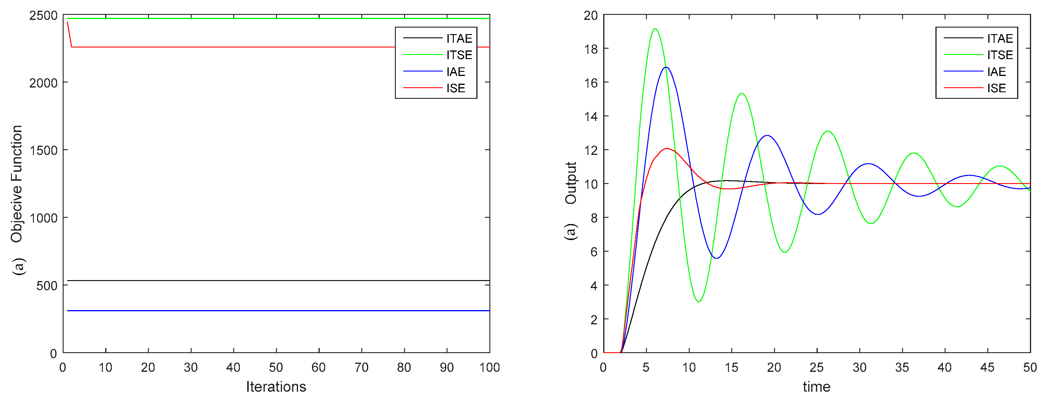
7], to optimize PID controller gains. BB–BC optimization algorithm is used to minimize performance control measures, integral absolute error (IAE), integral time absolute error (ITAE), integral square error (ISE), and integral time square error (ITSE) while minimizing the system overshoot. The key idea of using BB–BC here can be explained as the transformation of a convergent solution to a chaotic state and then back to a single tentative solution point. BB–BC algorithm has been implemented in various engineering applications, especially where the computational time and convergence time are important factors [8]. Some representative optimization problems, where the efficiency of BB–BC has been demonstrated, are the following: optimal design of truss structures [9], Schwedler and ribbed domes [10], concrete retaining walls [11], fuzzy inverse controllers [12], and fuzzy PID controllers [13]. Moreover, BB–BC algorithm has been adopted in real-time applications where the optimization task is adaptive or must be solved in relatively small sampling intervals. Besides its low computational time and high global convergence speed, another advantage of BB–BC, especially important for auto-tuning processes, is that it does not need gradient information and therefore can operate to minimize naturally defined cost functions without complex mathematical operations.
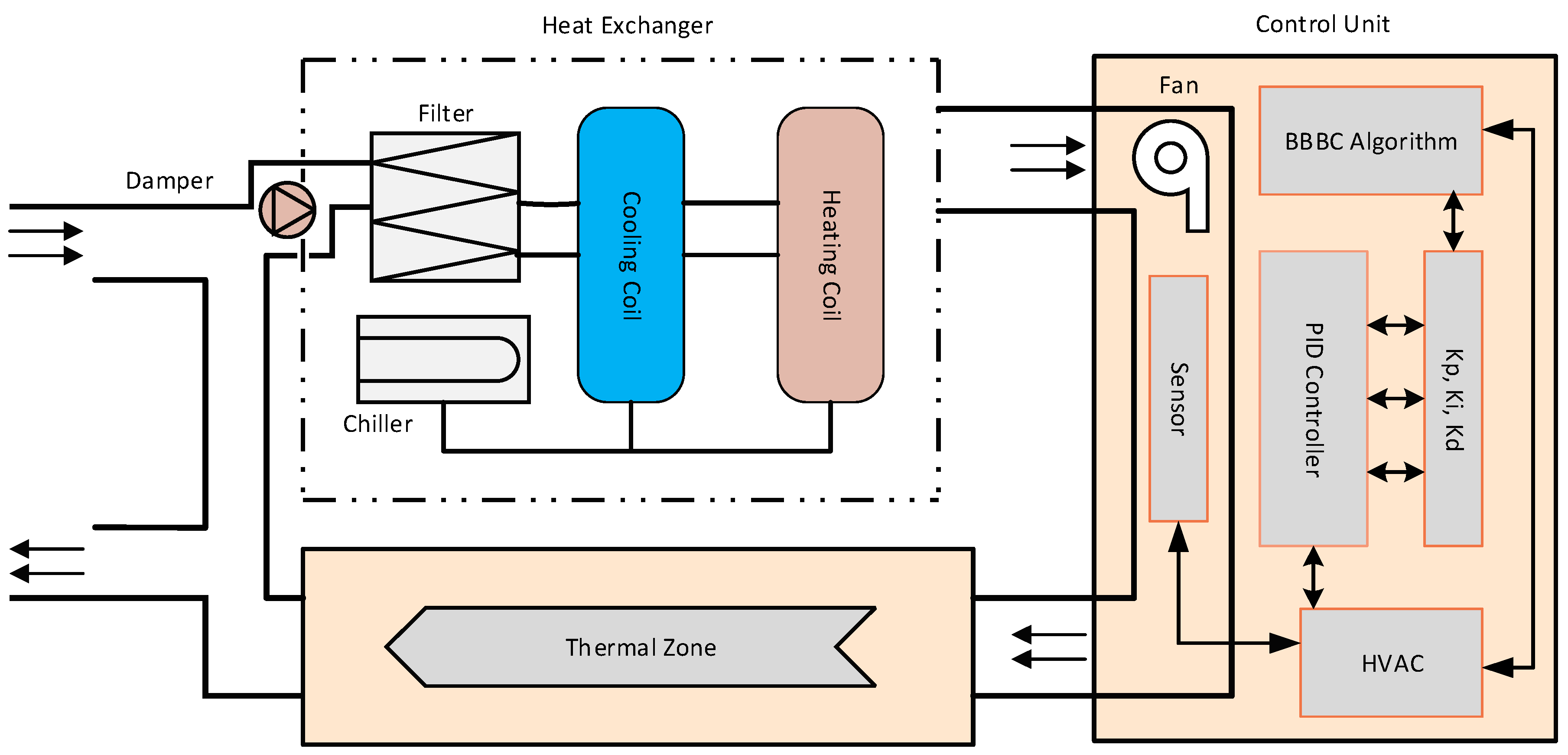
We evaluate the efficiency of BB–BC to tune the parameters of a PID controller used in a second-order heat, ventilation, and air conditioning (HVAC) system. In the HVAC system, the supply air pressure is regulated by the speed of a supply air fan. Increasing the fan speed will increase supply air pressure, and vice versa. The dynamics from the fan variable speed drive to the supply air pressure can be modeled as a second order plus dead time. This process is well established by Bi and Cai [14]. In real applications, however, where both fans and dampers exhibit non-linear properties for different working points, even a well-tuned PID controller may not be able to achieve a desired performance for all set points and process variations. Thus, we investigate how fast and accurate the BB–BC algorithm can tune the PID controller parameters in this HVAC system.
To further reduce the optimization latency of the control system, the BB–BC algorithm along with the PID controller, are accelerated using FPGA technology. Up to now, embedded computers, built around programmable microcontrollers, were the dominant computing platform for implementing PID controllers in industrial environments. The last decades, the field programmable hardware technology, also known as field programmable gate arrays (FPGAs), has emerged as an alternative solution for controlling industrial applications. The main advantages of the FPGA technology are reduced engineering cost, reduced time-to-market, high performance due to the exploitation of fine-grained hardware parallelism, and adaptation to control system requirements. Especially for control systems that use demanding computational intelligence techniques, the advanced performance of FPGAs combined with their low-cost and high adaptability render them an attractive computing platform. Taking also into consideration the real-time requirements of our HVAC system, we propose the FPGA-based acceleration of the BB–BC optimization algorithm and the PID controller to speed up the parameters tuning process, and consequently, improve system performance.
The BB–BC, PID controller and register transfer level (RTL) models have been described using the VHDL language and implemented in the Xilinx Zybo (Zynq) development board from Xilinx Corporation (San Jose, CA, USA). Built around the Xilinx Zynq XC7Z010 FPGA device. Moreover, the FPGA-in-the-loop (FIL) technique has been used to enable the emulation of the plant (HVAC) in MATLAB/Simulink environment in conjunction with the execution of the PID controller and the optimization process in the real hardware; this way, the FIL technique facilitates the evaluation of the entire system in higher abstraction layers [15].
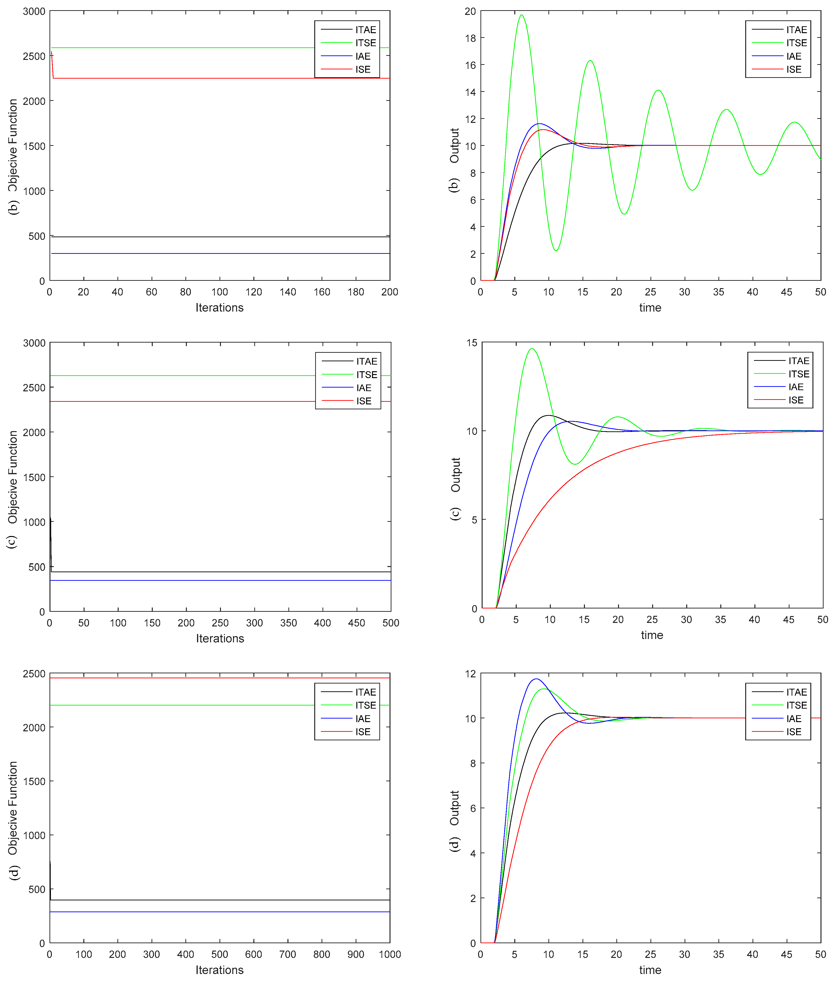
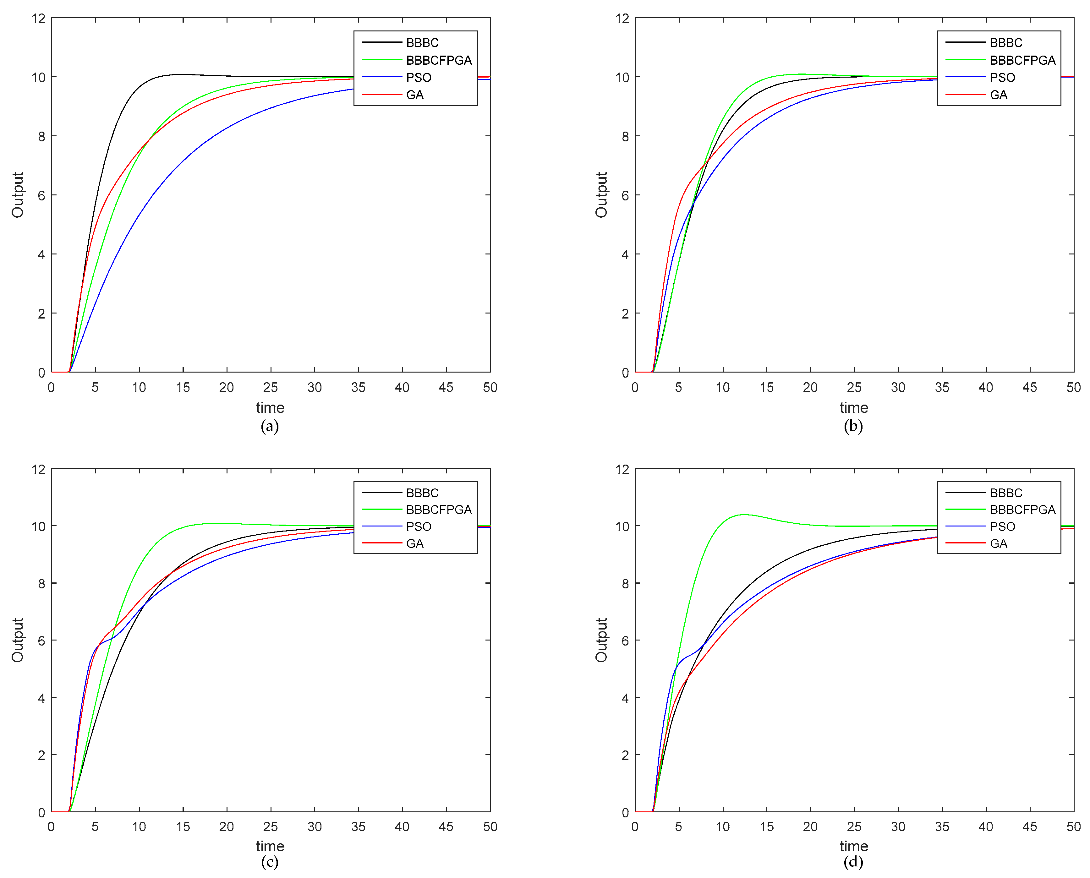
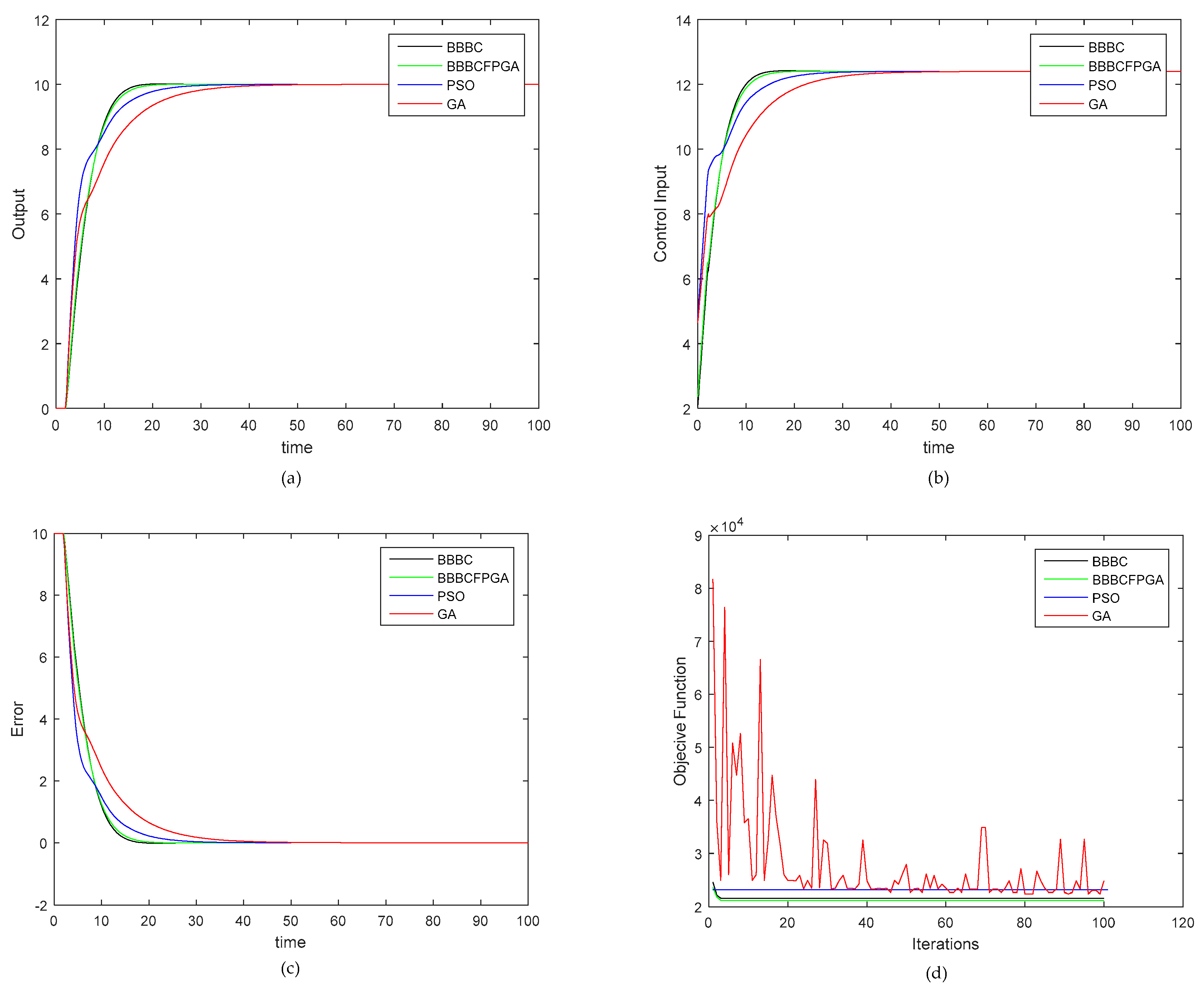
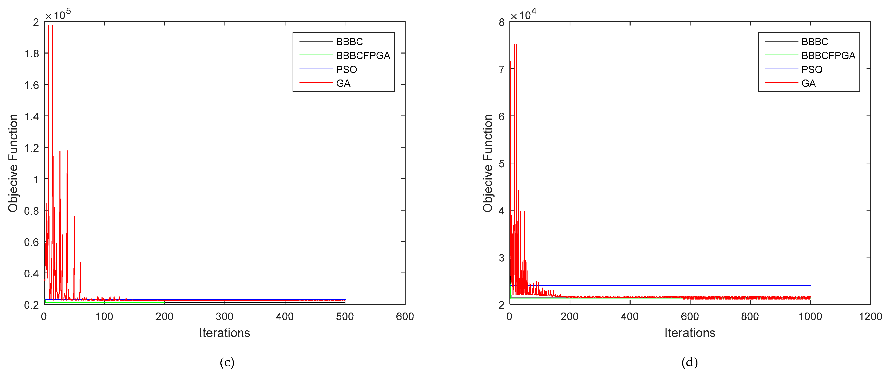
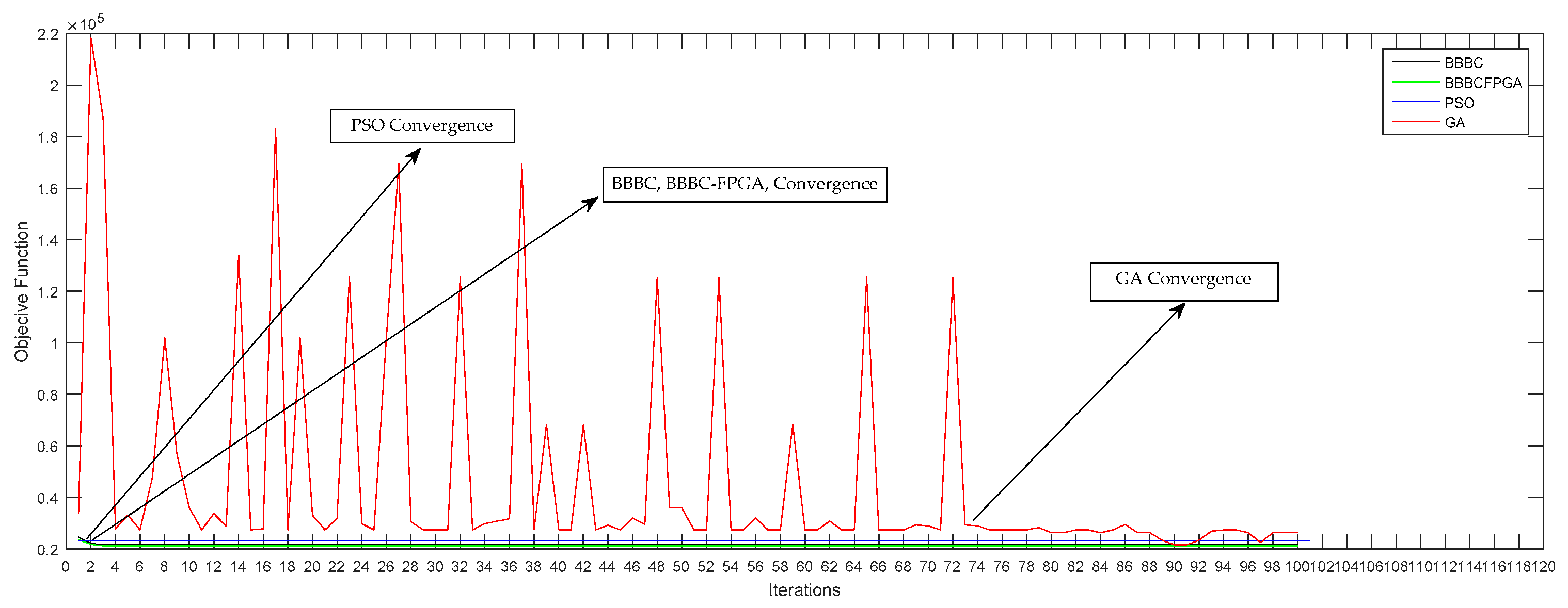
In order to demonstrate the efficiency of the proposed approach, we run various experiments in a second order system with two sec time delay and compared it with GA and PSO optimization algorithms in terms of PID tuning speed and convergence speed. The experimental results showed that the FPGA–BB–BC algorithm tunes the PID controller parameters ~430X faster than the software version of GA algorithm, ~539X faster than the software version of PSO algorithm, and ~270X faster than the software version of BB–BC algorithm. Furthermore, the proposed approach was tested under various fitness functions (error) for different number of iterations, and the integral time absolute error (ITAE) was chosen.
The organization of this paper is given as follows. Section 2 shortly describes the basics of PID controllers and BB–BC optimization algorithm. Section 3 presents the HVAC optimization problem and the proposed BB–BC-based tuning process of the PID parameters. Section 4 describes the FPGA implementation of the PID and BB–BC subsystems and the FIL approach. Section 5 presents the experimental results and demonstrates the efficiency of the proposed approach, while Section 6 concludes the paper.

2. Background

2.1. PID Controller

The PID controller has been widely used since its invention in 1910 in both academia and industry [16]. There are many PID control configurations, but the most common implementation is shown in Figure 1.
In general, the synthesis of the PID controller can be mathematically described by
u ( t ) = k p e ( t ) + k i 0 t e ( t ) d t + k d d d t e ( t )
where k p is the proportional gain, k d is the derivative gain, k i is the integral gain, and the error e ( t ) is the difference between the set-point and the plant output y(t). In addition, Equation (1) can be rewritten in Laplace form as
u ( s ) = e ( s ) [ k p + k i s + k d s ]
Finally, under the above scheme the transfer function of the PID controller or the control law is specified by
C ( s ) = u ( s ) e ( s ) = k p + k i s + k d s
For digital PID controllers, Equation (3) can be transformed via the z-domain into a difference equation for a recursive digital filter with an infinite impulse response (IIR) [16]
U ( z ) E ( z ) = k p + k i T s z z 1 + K d N ( z 1 ) ( 1 + N T s ) z 1
where T s is sampling period, N is the filter value.
To be implemented on an FPGA platform, a digital PID controller must be transformed to a difference equation, as shown below
U ( z ) E ( z ) = b 0 + b 1 z 1 + b 2 z 2 a 0 + a 1 z 1 + a 2 z 2
A differential equation can be derived from Equation (5) as follows
u [ n ] = k 1 u [ n 1 ] + k 2 u [ n 2 ] k 3 e [ n ] k 4 e [ n 1 ] k 5 e [ n 2 ]
Therefore, the relationship between the PID gains and its implementation in a digital system is shown in Table 1.
where the differential equation variables equal
a 0 = ( 1 + N T s ) a 1 = ( 2 + N T s ) ;   a 2 = 1 b 0 = k p ( 1 + N T s ) + k i T s ( 1 + N T s ) + k d N b 1 = ( k p ( 2 + N T s ) + k i T s + 2 k d N ) b 2 = k p + k d N

2.2. Big Bang–Big Crunch Algorithm

Big Bang–Big Crunch (BB–BC) algorithm was introduced by Erol and Eksin in [7]. Its key concept has been inspired by the creation theory of the universe. It is mainly consisted of two stages: the Big Bang phase and the Big Crunch phase. In the Big Bang phase, the population is randomly generated and the fitness function values of the individuals are calculated. Then, the Big Crunch phase follows. This phase implements a convergence operator, called the center of mass, that has many inputs but only one output, which is extracted by calculating the center of mass. Here, the term ‘mass’ refers to the inverse of the fitness function value. The point representing the center of mass is denoted by x c and calculated according to
x c = i = 1 N 1 f i x i i = 1 N 1 f i
where x i is an individual (point) within an L-dimensional search space, f i is the fitness function value of this individual, and N is the size of the population generated in the Big Bang phase. After the Big Crunch phase, the algorithm creates new members to be used as the Big Bang of the next iteration according to the following formula
x n e w = x c + r l / k
where r is a random number with normal distribution, k is the number of Big Bang iterations, and l is a problem-dependent constant, l = a ( x m a x x m i n ) ; parameter α limits the search space, while x m a x and x m i n are the upper and lower values of the optimization function variables. After the second explosion, the center of mass is recalculated. These successive explosion and contraction steps are carried out repeatedly until a stopping criterion has been met. Since normally distributed numbers can exceed ±1, it is necessary to keep the candidate values within the predefined search space bounds [6].
The steps of the BB–BC algorithm implementation as follows:
  • Form an initial generation of N candidates in a random manner.
  • Calculate the fitness function values of all the candidate solutions. This step depends on the target optimization problem.
  • Find the center of mass according to Equation (8). Best fitness individual of each generation can be also chosen as the center of mass instead of using Equation (8) reducing the computation time.
  • Calculate new candidates around the center of mass using Equation (9). Notice that the random value added or subtracted to the center of mass decreases as the iterations elapse.
  • Return to Step 2 until stopping criteria have been met.
Figure 2 below shows the flow chart of BB–BC algorithm.

3. Proposed Approach

3.1. HVAC System and PID Controller

The HVAC systems are automatic systems that control and provide a comfortable environment in terms of temperature, humidity, ventilation, and other parameters (power consumption, pressure, time control). HVAC systems are equipped with various sensors to monitor these parameters (e.g., temperature and humidity sensors, anemometers for measuring the flow speed, etc.) and optimize system performance and power consumption. In an HVAC system, the PID controller can be used in the control loop of the supply air pressure [17]. Figure 3 shows the block diagram of a conventional single-zone HVAC system. The control inputs of the HVAC system are the air flow rate, which can be adjusted through a variable-speed fan, and the water flow rate from the chiller to the heat exchanger. The PID controller calculations adjust motor speed as necessary to maintain a set point compared to the system output signal.
For the HVAC system—such as valve and damper operation, ambient temperature, and flow rate—the motor speed should be adjusted to maintain a set point difference. The BBBC-PID system performance depends on its ability to maintain a set point and speedup action.
The tuning process in large HVAC systems is a hard and time consuming task [18,19] due to their non-linearity and time-variance characteristics. Consequently, tuning the PID controller of an HVAC system in order to achieve the optimum tracking control performance is a hard problem. Here, we propose the use of BB–BC algorithm and FPGA technology to tune the PID parameters, and thus speed up the re-tuning process of the HVAC system when needed.

3.2. Tuning of the PID Parameters Using BB–BC

Evolutionary algorithms can be applied for the tuning of PID controller gains/parameters to ensure optimal control performance at stable operating conditions. In this paper, the BB–BC algorithm is employed for the offline tuning of the PID parameters (kp, ki, kd) in the HVAC model. Figure 3 above shows how the control unit consisting of the BB–BC unit and the PID controller is connected in the HVAC system. First, the BB–BC unit produces initial candidates for the PID parameters in the target search space. Next, based on the calculation of the objective function, it produces new candidate solutions around the center of mass until the stop criteria is satisfied.
In the design methodology of a PID controller, one of the most important performance criterion is the difference (error) between the plant output and the set point signal. Using this error criterion as the fitness function of the optimization algorithm results in a small overshoot with a long settling time. In general, fitness functions are based on error equations. The following four equations, integral time absolute error (ITAE), integral time square error (ITSE), integral absolute error (IAE), and integral square error (ISE) indicate the most commonly used fitness functions:
I S E = e ( t ) 2 . d t
I A E = | e ( t ) | . d t
I T A E = t . | e ( t ) | d t
I T S E = t . [ e ( t ) 2 ] . d t
Fitness functions are not actually limited to the above equations. Engineers can provide custom fitness functions depending on the target design and control system. The overall performance (convergence speed and optimization accuracy) of evolutionary algorithms depends on the fitness function adopted to monitor the optimization search.
To choose the optimal fitness function, i.e., the objective function of the BB–BC algorithm, we performed a set of experiments for the four typical error equations. We executed the four formulas of the errors (ITAE, ITSE, IAE, and ISE) for different number of iterations, specifically for 100, 200, 500, and 1000 cycles, in order to evaluate the performance of the objective functions. In the objective function used, the added term of control output u × u T (where u T is the transpose of u) seeks to reduce the magnitude of the control signal. When the objective function includes the control signal term (u), the algorithm seeks to minimize it. Therefore, the term u × u T is equivalent to squaring every element in u. The objective function that achieved the best performance is the integral time absolute error (ITAE) with control signal (u) as reported below in the equation (17). The results of these experiments are shown in Table 2.
Figure 4 presents the convergence and time response of the PID controller using the four objective functions (ITAE, ITSE, IAE, ISE) for parameters tuning for different number of iterations (100, 200, 500, and 1000). The curves show how the fitness function response (error) changes during the optimization process of the PID controller using BB–BC algorithm. Among the four traditional objective functions, the integral time absolute error (ITAE) provides the minimum settling time, peak overshoot, and rise time.
As mentioned above, any objective function can be adopted to tune the PID parameters. However, it is hard to reduce the rise time without increasing overshoot. By reducing the rise time, the system will try to follow the set-point faster, which will produce a greater inertia, thus raising the chance of an increased overshoot. As can be seen in Figure 4, although the response signal of ITAE declines faster, the convergence velocity of ITAE is obviously the best one compared with the other methods. Note that the integral absolute error (IAE) provides the best convergence, but its time response (overshoot, rise time, and settling time) is not optimal. Thus, in all cases (number of iterations), the integral time absolute error (ITAE) provides the best solution.

4. FPGA Implementation of PID Controller and BB–BC

The FPGA technology provides an effective solution in several industrial control applications due to its low development cost, high flexibility, and limited power consumption, while it has been proved an ideal processing platform for industrial applications with real-time constraints due to the acceleration achieved by the hardware parallelism. In this paper, we propose the use of FPGA technology to implement the BB–BC algorithm that calculates and optimizes the PID control parameters, (kp, ki, kd) in order to accelerate the control system process, which can be very effective for latency-sensitive applications.

4.1. PID Controller in FPGA

In the past, several approaches have proposed the use of FPGA technology to implement PID controllers [20,21] and/or optimize the PID controller parameters in real-time industrial applications, such as DC motor speed control system [22]. In [23], a fuzzy logic controller has been implemented on an FPGA platform and validated on a real-time application, namely a truck backer-upper control system. In [24], the authors presented a runtime reconfigurable PID controller that can dynamically switch between the different controller variants, e.g., PI, PD, PI-PD, etc., as the control requirements change.
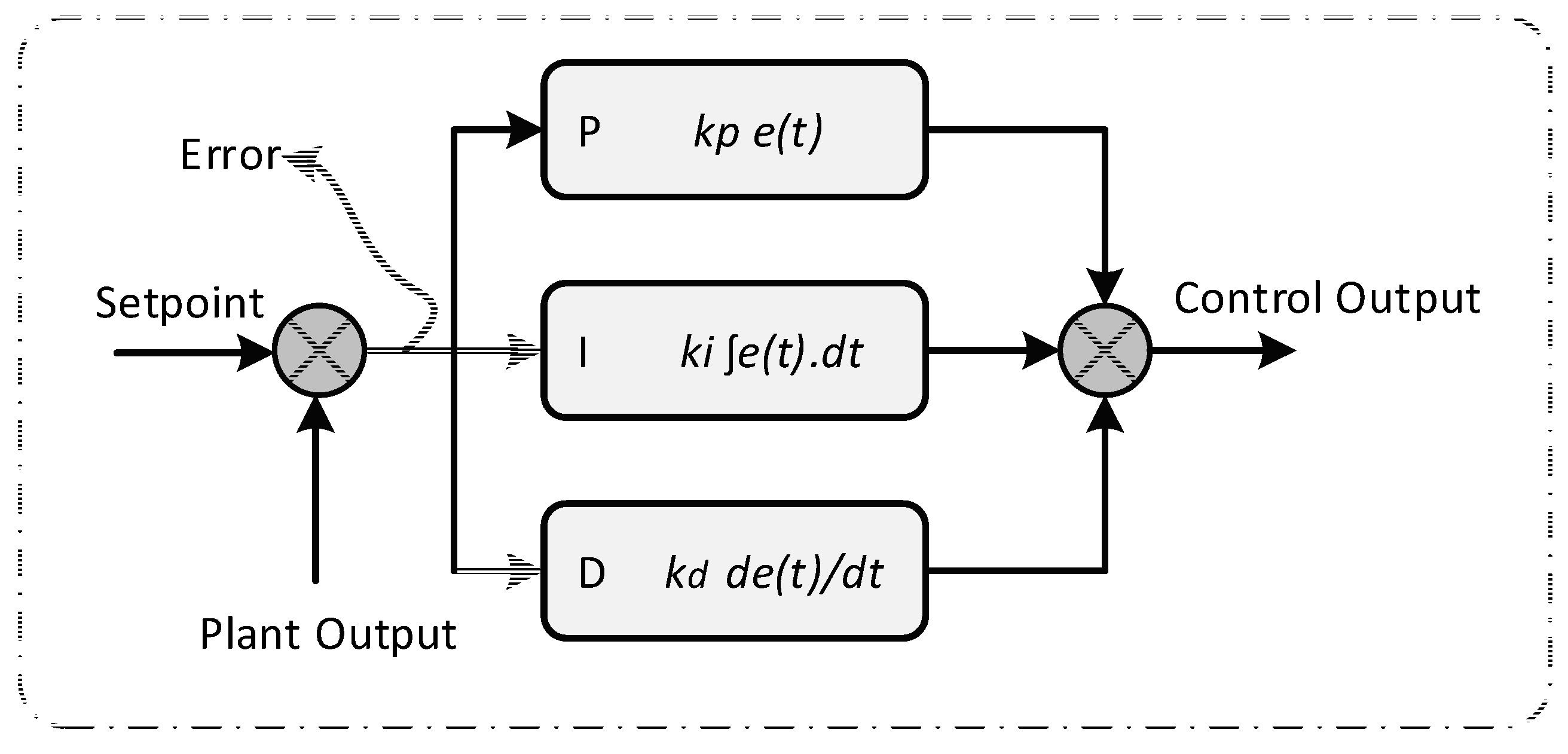
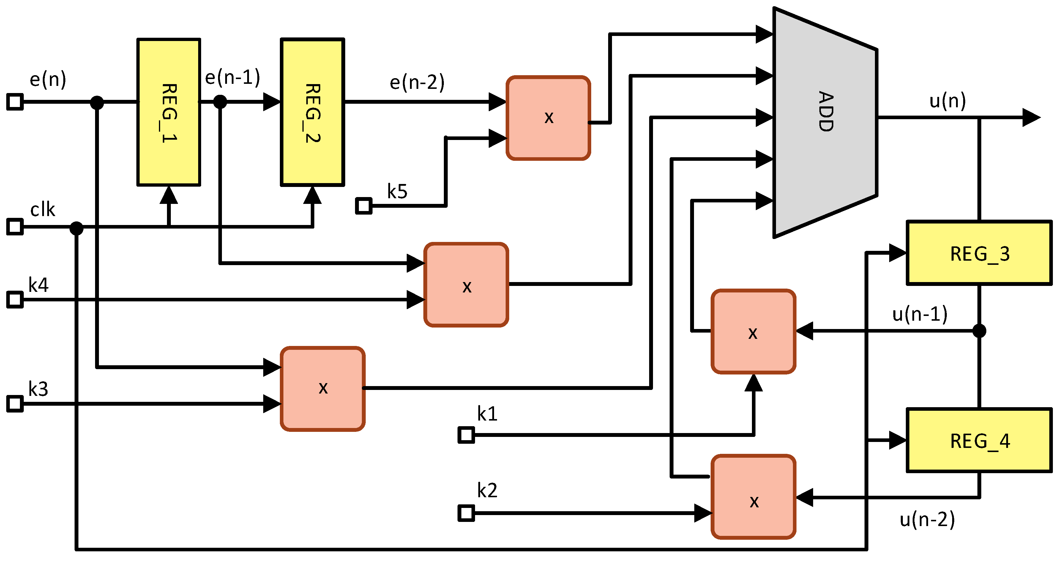
Figure 5 shows the block diagram of a typical PID controller FPGA architecture based on the differential Equation (6) and the parameters of Table 1.
The PID controller architecture consists of five registers blocks, for storing the current and previous error values, i.e., e(n), e(n − 1), e(n − 2), u(n − 1), and u(n − 2). Notice that the PID controller has a five-stage pipeline structure in order to increase clock frequency. Five arithmetic multipliers are used to multiply the proportional part, derivative part integral part with the corresponding parameters ( k 3 , k 4 , and k 5 , respectively) and the output signal with ( k 1 and k 2 ) as described in Table 1, while the adder finally sums all factors. Embedded DSP slices of the FPGA device are used for the implementation of arithmetic multipliers and adders in order to improve the design area and speed.

4.2. BB–BC Algorithm in FPGA

Several FPGA-based implementations of evolutionary algorithms have been presented in the literature to accelerate the optimization process. Most of these approaches focus on the optimal design of hardware accelerators to achieve high performance and flexibility [25,26] and satisfy other genetic algorithm features, such as multi-objective optimization [27]. In our approach, we adopted the BB–BC optimization algorithm due to its low computational time and high global convergence speed. These features of the BB–BC algorithm mainly motivated our work, since an FPGA-based BB–BC accelerator can greatly reduce the computational time providing an ideal platform for large-scale adaptive or latency-sensitive optimization problems [28].
In this subsection, we describe the FPGA design architecture of the BB–BC algorithm. 
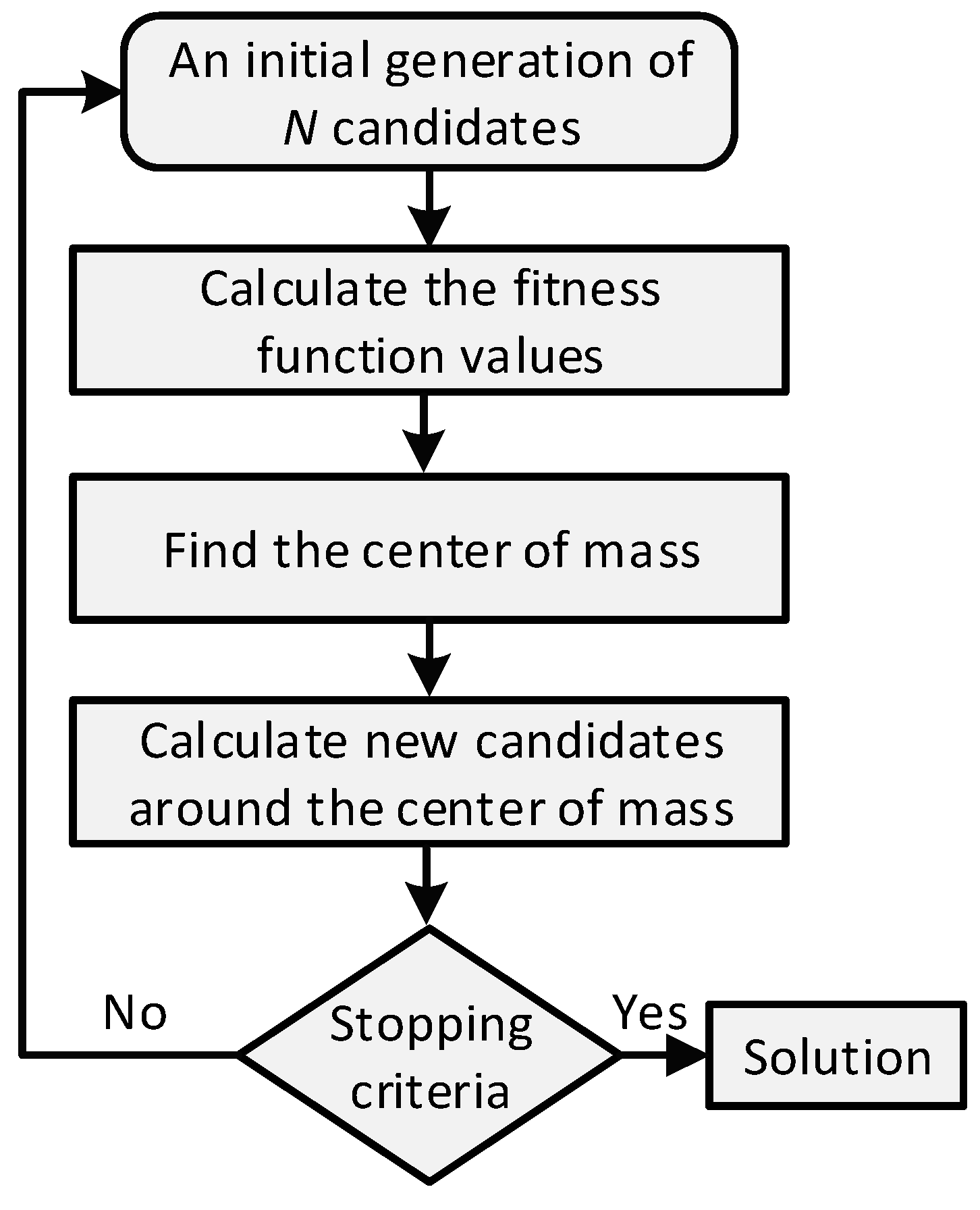
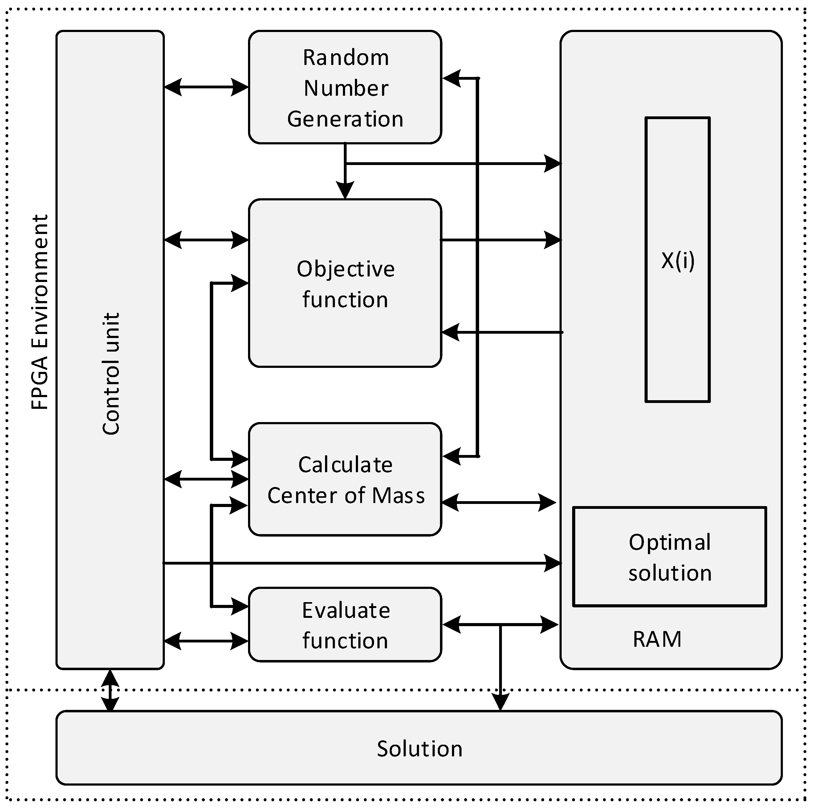
Figure 6 depicts the top-level design diagram of the FPGA BB–BC architecture consisting of the following blocks:
  • Random Number Generation: It generates the random numbers ( x i ), either to form an initial population (iteration 0) or to form new candidates around the CoM (iteration > 0). A typical linear feedback shift register (LFSR) is used to generate random numbers based on a configurable seed. Note that the boundaries of the random numbers are determined by the upper and lower values of the optimization function variables. In each iteration, the module generates N candidates sequentially, where N is the population size, with each one consisting of L random numbers, where L is the number of features of each candidate. The generated random numbers of each iteration are stored in a RAM in order to be processed later for the calculation of center of mass.
  • Objective Function: After the random number generation, this module calculates the objective function ( f i ) for each candidate ( x i ) using the ITAE equation, which is also stored in the RAM. Both the random number generation and objective function modules have been implemented following a simple, serial processing model, where a single element is processed in each clock cycle, providing a low-cost FPGA circuit. Note that both modules can be parallelized (i.e., to generate the random numbers and calculate the objective functions concurrently using many processing elements working in parallel) and pipelined in order to improve performance, as proposed in [28].
  • Calculate Center of Mass: It reads the candidates and their objective function values from the RAM and calculates the center of mass which is forwarded in the random number generation module to generate the population in the next iteration cycle.
  • Evaluate Function: It reads the objective function values of the candidates from the RAM in order to select the best fitness candidate which is store in RAM too, and from output signal when the FPGA-BBBC control the HVAC model.
  • Control Unit: It orchestrates the operation of the other modules and repeats the BB–BC steps until the stopping criteria are met.
  • Solution: It includes a register that stores the outcome of the BB–BC algorithm.
Note that a high-performance FPGA architecture of BB–BC algorithm has been presented in [28] which incorporates parallel pipelined engines to accelerate the execution of BB–BC. This FPGA BB–BC architecture has been optimized in terms of execution latency and is very suitable for control applications with strict real-time requirements. However, this performance optimization has been achieved at the expense of extra hardware area and power consumption. Thus, the optimized FPGA architecture of [28] is suggested only for time sensitive control applications.
Table 3 presents the device utilization summary on a Xilinx Zynq XC7Z010 FPGA device.

4.3. FPGA-In-The-Loop (FIL)

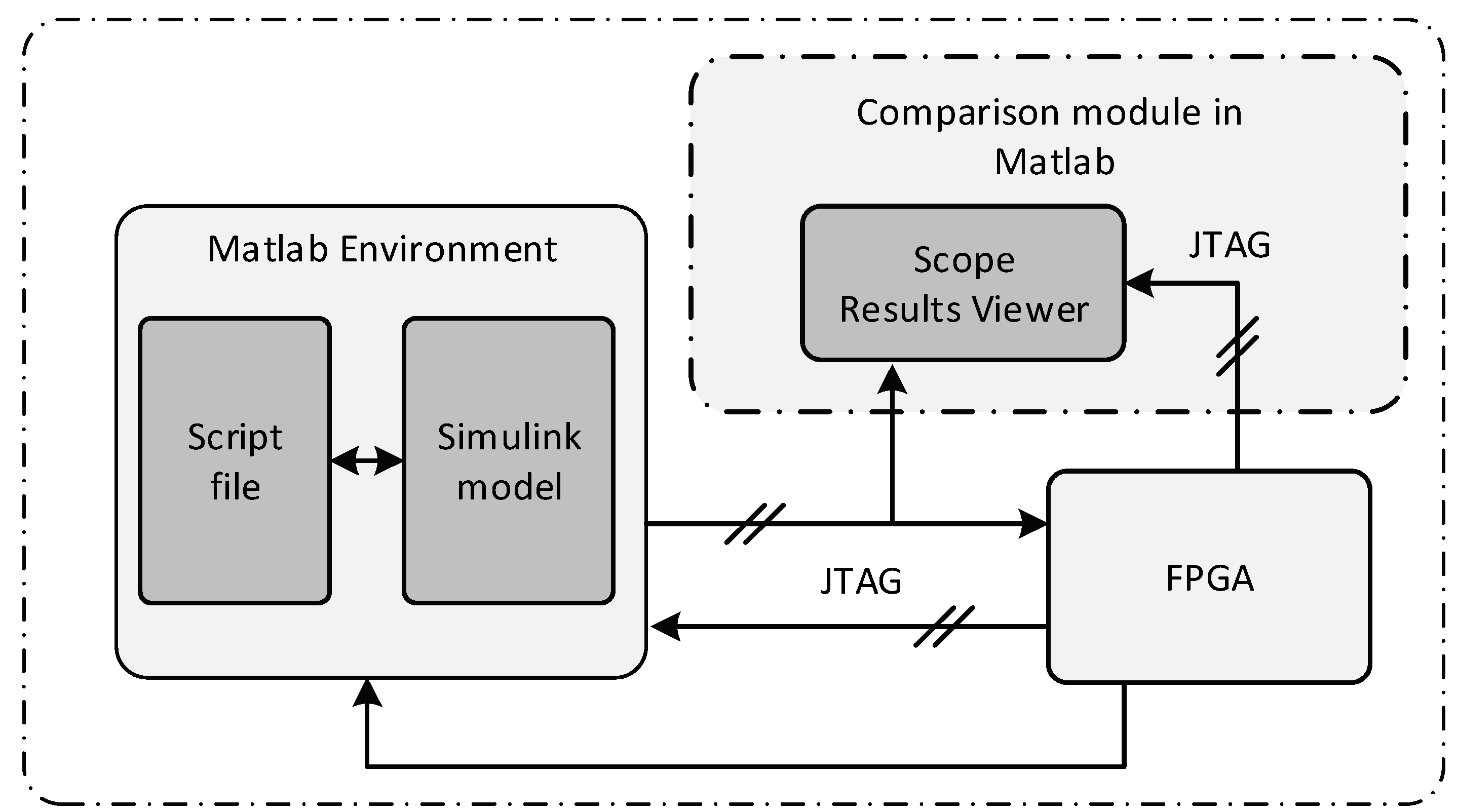
MATLAB/Simulink is a high-level language and interactive environment highly popular among system and algorithm designers for many different real-world applications and research topics. To accommodate developers to interface with real hardware (e.g., components implemented in FPGA devices), MathWorks® presented the FPGA-in-the-loop (FIL) concept. Based on this idea, data can be exchanged between the MATLAB/Simulink modules and the FPGA device. FIL scheme can be used for multiple tasks while designing, evaluating, and verifying designs. For example, it can be used to configure and tune FPGA design parameters at runtime, such as tuning data pipe gains and modifying filter parameters [29], or to monitor hardware components by reading specific status registers at runtime. Another powerful capability of the FIL approach is that allows the generation of complex stimulus datasets on the host PC and rapid download to the FPGA target in real time [29]. By using the FIL approach and connecting the hardware target via some common protocol interface (e.g., Ethernet or JTAG), one can obtain significant improvements in simulation runtime compared to cycle-accurate host simulation.
As shown in Section 5, the proposed approach in conjunction with the FIL technique achieves a speedup of around 253X compared to the MATLAB 2015b software simulation. Moreover, when design complexity increases, the advantages of the FIL methodology over software simulation at runtime will be more evident. Figure 7 presents the structure of the FIL acceleration scheme used in our system, where MATLAB/Simulink provides the user with a working environment.

4.4. System Architecture

The FPGA design consisting of the PID controller and the BB–BC algorithm is written in VHDL hardware description language and implemented in a Xilinx development platform, Zybo–7010 board, using the Xilinx ISE Design Suite 14.7 and Vivado Design Suite. 
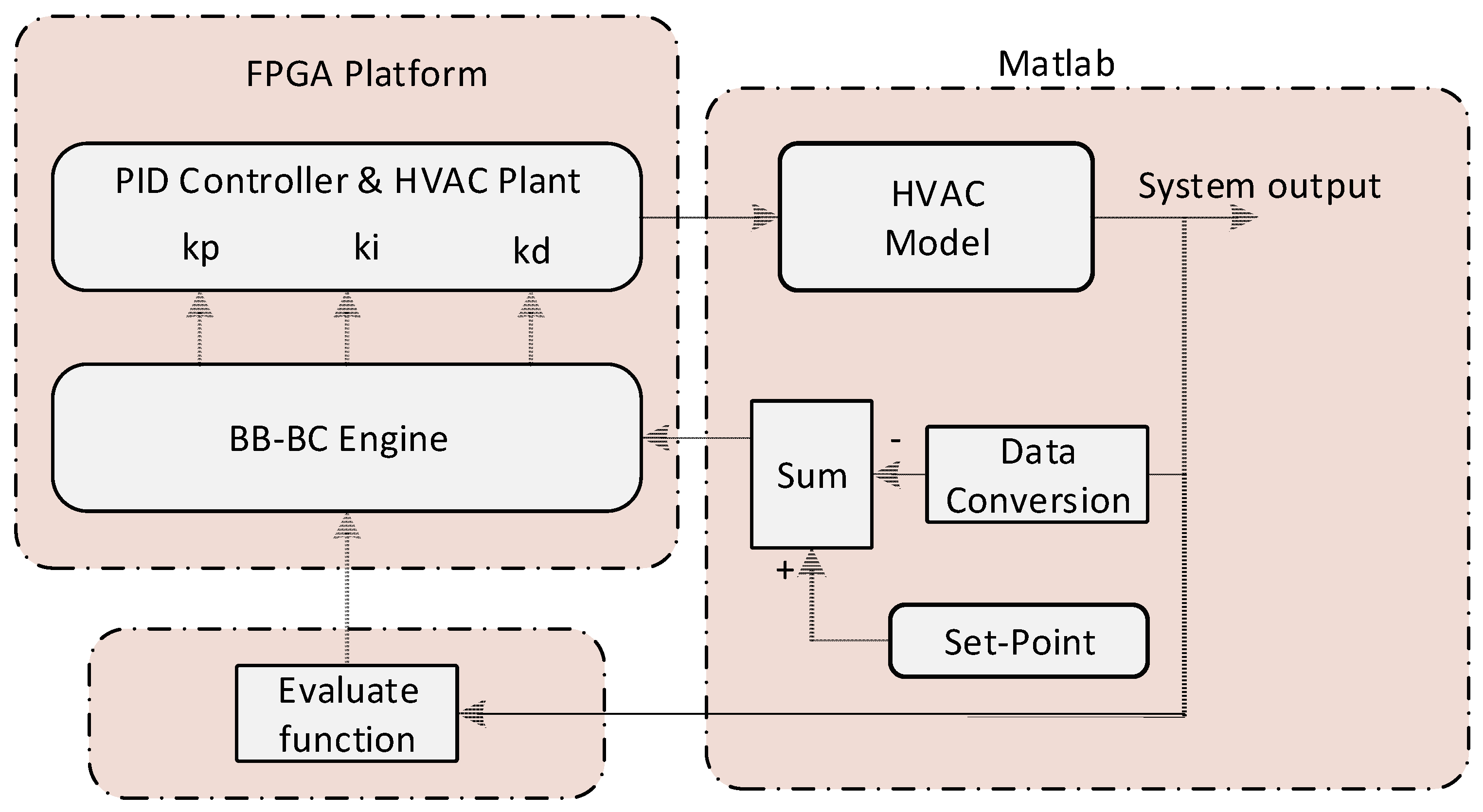
Figure 8 depicts the entire system architecture including the FPGA device and the HVAC model implemented in MATLAB environment. The processing steps of the proposed architecture are shortly described below.
(1)
The FPGA BB–BC module generates a set of random PID parameters (kp, ki, kd), either to form the initial candidate or the new candidate around the center of mass in the next iteration cycles.
(2)
The FPGA PID controller module receives the values of the parameters and controls the HVAC plant.
(3)
The FPGA BB–BC module calculates the fitness functions for this candidate (i.e., PID parameters) using the ITAE equation and then calculates the new center of mass.
(4)
The HVAC model runs for a short period.
(5)
The evaluate function checks the system output and decides whether the BB–BC module must re-run to improve system performance, i.e., when the system has been affected by external disturbances that cause the output to exceed some predefined thresholds. Note that we use the HVAC plant as a part of the FPGA BBBC module to produce the first optimization parameters (kp, ki, kd) of the PID controller for the HVAC model in the first run.
Given that the evolutionary algorithms consume enough time to reach the optimal solution, even when the number of iterations is small, they are not suitable for latency-sensitive applications in real time. However, accelerating the evolutionary algorithm using an FPGA-based platform, as in the case of FPGA-in-the-loop (FIL) paradigm, can reduce the execution time and achieve the convergence into the optimal solution under specific timing constraints. Therefore, the FPGA-based BB–BC algorithm can be executed much faster, fact that improves confidence that the target optimization algorithm can finally satisfy the real-time requirements of an industrial application.
The total execution time of the MATLAB/Simulink model ( T M S ) incorporates the MATLAB processing time, the FPGA execution time and the time required for the data exchange between the host PC and the FPGA board and is given by the equation
T M S = T M P + T M 2 F + ( T F P G A ) + T F 2 M
where T M S is total execution time of the MATLAB/Simulink model, T M P is the MATLAB processing time, T M 2 F is the time required for transferring data from MATLAB to FPGA platform, T F P G A is the FPGA processing time, and T F 2 M is the time required for copying data from FPGA platform to the MATLAB/Simulink environment.
Assuming population size N and number of iterations M, the total execution time ( T F P G A ) of the proposed FPGA BB–BC circuit is given by the equation
T F P G A = M × N × ( T C G + T F C + T C O M + T P I D + P l a n t )
where T C G ,   T F C ,   T C O M are the latencies of the FPGA BB–BC stages, i.e., candidate generation, fitness function calculation, and center of mass calculation, respectively and T P I D + P l a n t is the latency of FPGA PID controller and the plant.
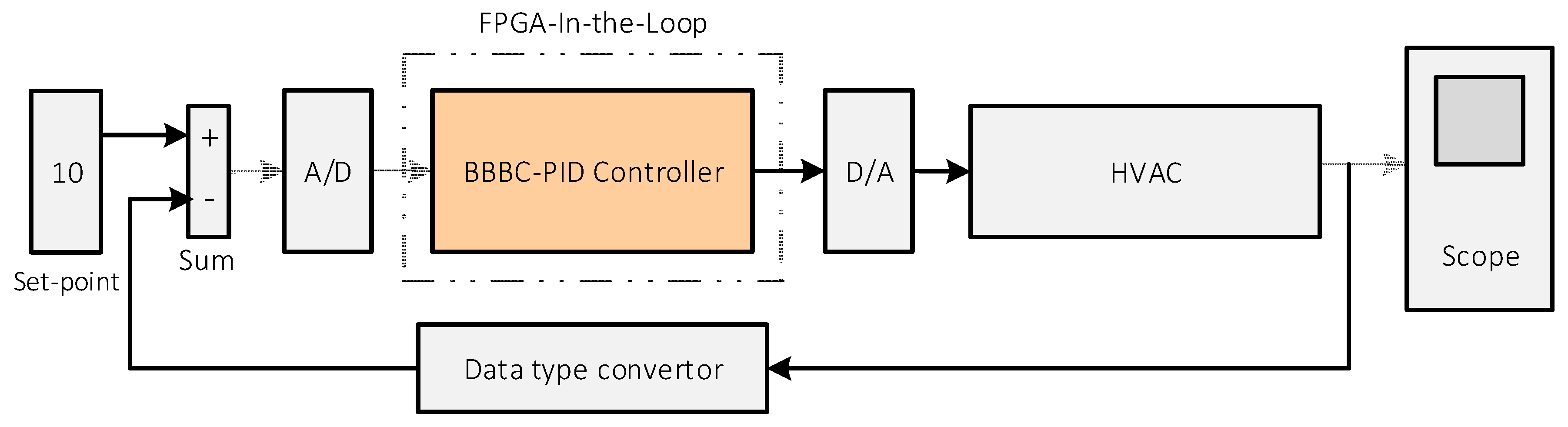
Figure 9 shows the top-level diagram of our MATLAB/Simulink model, which includes the FPGA BB–BC/PID module (using the FIL concept), the HVAC module, an analog-to-digital converter to feed the digital error value into the FPGA BB–BC module, an digital-to-analog converter to provide the PID controller output to the HVAC model, an adder to calculate the error and the set point.

5. Experiments on the HVAC System

The efficiency of the proposed approach was demonstrated by a set of experimental tests performed over a second order system with two seconds delay.
In our case study (HVAC) simulation experiments, we observed that, when BB–BC runs and the error value is calculated in the beginning, the plant output becomes equals to set point, while when the optimal values for k P , k i , and k d are used to calculate the current plant output, the plant output equals the set point when error reaches near to zero, hence plant starts running at the set point. The final outputs of the proposed design are the optimized PID controller parameters ( k P , k i , k d ) used in the HVAC control system. The experiments showed that our approach considerably reduces the overshoot value without compromising the latency sensitivity compared to the genetic and particle swarm optimization algorithms where the desired overshoot is not considered, even when the error and response time is reduced [30].

5.1. Experimental Setup

In the HVAC systems, the air pressure supplier is regulated by the speed of the air fan. Increasing the fan speed we manage to increase the supply air pressure, and vice versa. The dynamics system from the control signal output u(t) that providing to the fan variable speed drive to the supply air pressure can be modeled as a second-order added time-delay system. The process response is shown in Figure 3. For our experiments, we have adopted the HVAC model proposed in [14]. In [14], the authors derived this HVAC model after various experimental tests on supply air pressure and room pressure in an HVAC pilot. Thus, our target system is an HVAC model using the transfer function
G ( s ) = e 2 s 0.12 s 2 + 1.33 s + 1.24
The system response performance criterion used as objective function in our optimization algorithm is the integral time absolute error (ITAE) plus the control signal (u) given by the formula
I T A E = t . | e ( t ) | d t + u T u
Note that integral time absolute error (ITAE) is widely used in control processing since it is simple to implement and natural to define energy of a signal, which possesses symmetry and differentiability.

5.2. System Performance and Convergence

In order to evaluate the robustness of the proposed approach against other optimization methods we simulated our HVAC model running: (i) BB–BC algorithm in MATLAB sw, (ii) BB–BC in FPGA (our approach), (iii) PSO method in MATLAB sw and (iv) GA in MATLAB sw. The simulation is performed for different number of iterations (M = 100, 200, 500, 1000) and the results are illustrated in Figure 10.
The BB–BC, PSO, and GA models run in a Core i7-3612QM@ 2.10 GHz (64-bit) processor. The transient performance measured in seconds is presented in Table 4, while Figure 11 shows the control system action, i.e., system output, control signal, error, and objective function for all optimization methods, assuming population size (N = 10) and number of iterations (M = 100). As it can be clearly, the BBBC-FPGA approach is more robust compared to both PSO and GA approaches.
Figure 12 shows the best values of objective function per iteration for all four optimization algorithms for different number of iterations. In all cases, BBBC and BBBC-FPGA converge faster (locally minima) than GA and PSO, mostly expected from the BB–BC algorithm literature.
With a new run of all optimization methods, Table 5 and Figure 13 provide more details about the objective function convergence presented on Figure 12 including the number of iterations, the steady state time (SST) and the running time assuming population size (N) equals 10 and number of iterations (M) equals 100.

5.3. Computation Time

Table 6 compares the computation time of the proposed approach (BBBC-FPGA) with GA and BB–BC implemented in software (MATLAB model). The proposed approach achieves a speedup of more than 428X compared to the GA (in sw) approach and more than 253X compared to the BBBC (in sw) approach.

6. Conclusions

In this paper, we presented a novel technique for the fast tuning of the parameters of the PID controller of a second-order heat, ventilation, and air conditioning (HVAC) system using a low-cost, fast-convergent optimization algorithm, called Big Bang–Big Crunch (BB–BC). To further accelerate the optimization process, we proposed the implementation of both the BB–BC algorithm and the PID controller using FPGA technology. In order to emulate and evaluate the entire system we adopted the FPGA-in-the-loop (FIL) technique, according to which, the plant (i.e., MATLAB/Simulink model of HVAC) is connected to the FPGA board (i.e., the PID and BB–BC modules). To demonstrate the efficiency of the proposed approach, we run an extensive set of experiments in a second-order HVAC model using different optimization methods (BB–BC in FPGA, BB–BC in sw, GA, and PSO in sw). The experimental results proved the benefits of the proposed approach against the other methods in terms of convergence speed and computation time.

Author Contributions

The contributions of all authors are equals. All authors have worked together to develop and approved the manuscript. A.D., M.P. are the research advisors, who helped in proofreading and improving the quality of the final version of the manuscript.

Acknowledgments

The gratefully acknowledges the helpful comments and suggestions of both reviewers, which have improved the manuscript.

Conflicts of Interest

The authors declare no conflict of interest.

Abbreviations

ADDAdder
BB-BCBig Bang-Big Crunch
ClkClock
CoMCenter of Mass
DEDeferential Equation
FILField programmable gate array in the Loop
FPGAField Programmable Gate Array
GAGenetic Algorithm
HVACHeat Ventilation Air Condition
IAEIntegrated Absolute Error
ISEIntegrated Square Error
ITAEIntegrated Time Absolute Error
ITSEIntegrated Time-weighted Square Error
PIDProportional Integrating Derivative
PSOParticle Swarm Optimization
RandGenRandom Generator
REGRegister
RTRunning Time
RTLRegister Transfer Level
SSTSteady State Time
VHDLVery High Speed Integrated Circuit Hardware Description Language

References

  1. Cominos, P.; Munro, N. PID Controllers: Recent Tuning Methods and Design to Specification. IEEE Proc. Control Theory Appl. 2002, 149, 46–53. [Google Scholar] [CrossRef]
  2. Li, Y.; Ang, K.H.; Chong, G. PID control system analysis and design. IEEE Control Syst. Mag. 2006, 26, 32–41. [Google Scholar] [Green Version]
  3. Kumar, R.A.; Daya, J.L.F. A Novel Self-Tuning Fuzzy Based PID Controller for Speed Control of Induction Motor Drive. In Proceedings of the International Conference on Control Communication and Computing, Thiruvananthapuram, India, 13–15 December 2013. [Google Scholar]
  4. Xu, J.X.; Huang, D. Optimal Tuning of PID Parameters Using Iterative Learning Approach. In Proceedings of the IEEE 22nd International Symposium on Intelligent Control, Singapore, 1–3 October 2007; pp. 226–231. [Google Scholar]
  5. Mitsukura, Y.; Yamamoto, T.; Kaneda, M. A design of self-tuning PID controllers using a genetic algorithm. In Proceedings of the American Control Conference, San Diego, CA, USA, 2–4 June 1999; pp. 1361–1365. [Google Scholar]
  6. Chung, I.-Y.; Liu, W.; Cartes, D.A.; Schoder, K. Control parameter optimization for a microgrid system using particle swarm optimization. In Proceedings of the IEEE International Conference on Sustainable Energy Technologies, Singapore, 24–27 November 2008; pp. 837–842. [Google Scholar]
  7. Osman, E.; Eksin, I. New optimization method: Big Bang-Big Crunch. Adv. Eng. Softw. 2006, 37, 106–111. [Google Scholar]
  8. Kumbasar, T.; Hagras, H. Big Bang–Big Crunch optimization based interval type-2 fuzzy PID cascade controller design strategy. Inf. Sci. 2014, 282, 277–295. [Google Scholar] [CrossRef]
  9. Kaveh, A.; Talatahari, S. Size optimization of space trusses using Big Bang–Big Crunch algorithm. Comput. Struct. 2009, 87, 1129–1140. [Google Scholar] [CrossRef]
  10. Kaveh, A.; Talatahari, S. Optimal design of Schwedler and ribbed domes via hybrid Big Bang–Big Crunch algorithm. J. Constr. Steel Res. 2010, 66, 412–419. [Google Scholar] [CrossRef]
  11. Camp, C.V.; Akin, A. Design of retaining walls using big bang–big crunch optimization. J. Struct. Eng. 2011, 138, 438–448. [Google Scholar] [CrossRef]
  12. Kumbasar, T.; Eksin, I.; Guzelkaya, M.; Yesil, E. Adaptive fuzzy model based inverse controller design using BB-BC optimization algorithm. Exp. Syst. Appl. 2011, 38, 12356–12364. [Google Scholar] [CrossRef]
  13. Yesil, E. Interval type-2 fuzzy PID load frequency controller using Big Bang–Big Crunch optimization. Appl. Soft Comput. 2014, 15, 100–112. [Google Scholar] [CrossRef]
  14. Bi, Q.; Cai, W.-J. Advanced controller auto-tuning and its application in HVAC systems. Control Eng. Pract. 2000, 8, 633–644. [Google Scholar] [CrossRef]
  15. Ządek, P.; Koczor, A.; Gołek, M.; Matoga, L.; Penkala, P. Improving Efficiency of FPGA-in-the-Loop Verification Environment. IFAC-PapersOnLine 2015, 48, 180–185. [Google Scholar] [CrossRef]
  16. Astrom, K.J.; Hagglund, T. PID Controllers Theory, Design, and Tuning, 2nd ed.; Instrument Society of America: Research Triangle Park, NC, USA, 1995. [Google Scholar]
  17. Maasoumy, M.; Sangiovanni-Vincentelli, A. Total and peak energy consumption minimization of building HVAC systems using model predictive control. IEEE Des. Test Comput. 2012, 29, 26–35. [Google Scholar] [CrossRef]
  18. Wang, L.; Du, W.; Wang, H.; Wu, H. Fuzzy Self-Tuning PID Control of the Operation Temperatures in a Two-Staged Membrane Separation Process. J. Nat. Gas Chem. 2008, 17, 409–414. [Google Scholar] [CrossRef]
  19. Dounis, A.I.; Caraiscos, C. Advanced control systems engineering for energy and comfort management in a building environment—A review. Renew. Sustain. Energy Rev. 2009, 13, 1246–1261. [Google Scholar] [CrossRef]
  20. Lima, J.; Menotti, R.; Cardoso, J.; Marques, E. A methodology to design FPGA-based PID controllers. In Proceedings of the 2006 IEEE International Conference on Systems, Man and Cybernetics, Taipei, Taiwan, 8–11 October 2006. [Google Scholar]
  21. Chan, Y.; Wang, W.; Moallem, M. Design and Implementation of Modular FPGA-Based PID Controllers. IEEE Trans. Ind. Electron. 2007, 54, 1898–1906. [Google Scholar] [CrossRef] [Green Version]
  22. Sonoli, S.K.; Nagabhushan, R. Implementation of FPGA based PID Controller for DC Motor Speed Control System. In Proceedings of the World Congress on Engineering and Computer Science, San Francisco, CA, USA, 20–22 October 2010. [Google Scholar]
  23. Kim, D. An implementation of fuzzy logic controller on the reconfigurable FPGA system. IEEE Trans. Ind. Electron. 2000, 47, 703–715. [Google Scholar]
  24. Khan, S.; Papadimitriou, K.; Buttazzo, G.; Kalaitzakis, K. A Reconfigurable PID Controller. In Proceedings of the 14th International Symposium, ARC 2018, Applied Reconfigurable Computing, Architectures, Tools, and Applications, Santorini, Greece, 2–4 May 2018. [Google Scholar]
  25. Tang, W.; Yip, L. Hardware implementation of genetic algorithms using FPGA. In Proceedings of the 47th Midwest Symposium on Circuits and Systems, Hiroshima, Japan, 25–28 July 2004; pp. 549–552. [Google Scholar]
  26. Shackleford, B.; Snider, G.; Carter, R.J.; Okushi, E.; Yasuda, M.; Seo, K.; Yasuura, H. A high-performance, pipelined, FPGA-based genetic algorithm machine. Genet. Program. Evolv. Mach. 2001, 2, 33–60. [Google Scholar] [CrossRef]
  27. Tachibana, T.; Murata, Y.; Shibata, N.; Yasumoto, K.; Ito, M. A hardware implementation method of multi-objective genetic algorithms. In Proceedings of the IEEE Congress on Evolutionary Computation, Vancouver, BC, Canada, 16–21 July 2006; pp. 3153–3160. [Google Scholar]
  28. Almabrok, A.; Psarakis, M.; Anastasios, D. An Efficient FPGA Implementation of the Big Bang-Big Crunch Optimization Algorithm. In Proceedings of the 14th International Symposium, ARC 2018, Applied Reconfigurable Computing, Architectures, Tools, and Applications, Santorini, Greece, 2–4 May 2018. [Google Scholar]
  29. Altera. Hardware in the Loop from the MATLAB/Simulink Environment. Available online: https://www.altera.com/en_US/pdfs/literature/wp/wp-01208-hardware-in-the-loop.pdf (accessed on 22 January 2017).
  30. Pal, A.; Mudi, R. Self-Tuning Fuzzy PI Controller and its Application to HVAC Systems. Int. J. Comput. Cogn. 2008, 6, 25–30. [Google Scholar]
Figure 1. Block diagram of typical PID control structure.
Algorithms 11 00146 g001
Figure 2. BB–BC optimization algorithm flow chart.
Algorithms 11 00146 g002
Figure 3. Block diagram of conventional HVAC system and control unit structure.
Algorithms 11 00146 g003
Figure 4. Convergence and time response of the widely used objective function in controller tuning via optimization (ITAE, ITSE, IAE, ISE) for different number of iterations (a) 100, (b) 200, (c) 500 and (d) 1000 iterations.
Algorithms 11 00146 g004aAlgorithms 11 00146 g004b
Figure 5. Block diagram of a typical PID controller FPGA architecture.
Algorithms 11 00146 g005
Figure 6. Top-level diagram of the BB–BC FPGA architecture.
Algorithms 11 00146 g006
Figure 7. FPGA-in-the-loop (FIL) acceleration scheme.
Algorithms 11 00146 g007
Figure 8. Proposed system architecture.
Algorithms 11 00146 g008
Figure 9. Block diagram of our MATLAB/Simulink model.
Algorithms 11 00146 g009
Figure 10. Time responses of four optimization methods (BBBC, BBBC-FPGA, PSO, GA) for different number of iterations (a, b, c, and d for 100, 200, 500, and 1000 iterations, respectively).
Algorithms 11 00146 g010
Figure 11. The (a) system output, (b) control signal, (c) error signal, and (d) objective function for all four optimization methods.
Algorithms 11 00146 g011
Figure 12. Objective function convergence for all four optimization methods and for different number of iterations (a, b, c, and d for 100, 200, 500, and 1000 iterations, respectively).
Algorithms 11 00146 g012aAlgorithms 11 00146 g012b
Figure 13. Objective function convergence for all four optimization methods.
Algorithms 11 00146 g013
Table 1. Equivalence of parameters for PID controllers
C(z)k1k2k3k4k5
C(z) a 1 a 0 a 2 a 0 b 0 a 0 b 1 a 0 b 2 a 0
Table 2. Comparison of different errors, ITAE, ITSE, IAE, ISE as performance index (fitness function).
Iteration No.ITAEITSEIAEISE
1005.33 × 1022.47 × 1033.10 × 1022.25 × 103
2004.85 × 1022.58 × 1032.99 × 1022.24 × 103
5004.40 × 1022.62 × 1033.46 × 1022.34 × 103
10003.96 × 1022.20 × 1032.86 × 1022.45 × 103
Table 3. Device utilization summary of the PID controller on a Xilinx Zynq FPGA device
Logic UtilizationUsedAvailableUtilization
Number of Slice Registers30654,5760%
Number of Slice LUTs16,99827,28862%
Number of Block RAM/FIFO21161%
Number of DSP48A1s545893%
Table 4. Transient performance comparison.
MethodPID ParametersOs %TsTr
kpkikd
BBBC0.2050.0630.0460.5058.6327.708
BBBC-FPGA0.2360.0760.0200.5059.4987.959
GA0.3410.1540.0140.49323.19614.014
PSO0.4790.2170.0060.49915.4309.364
Table 5. Objective function convergence details (iterations and execution time) for all four optimization methods
Tuning MethodConvergence IterationSteady State Time (s)Running Time (s)
BBBC210.6424.061
BBBC-FPGA211.4560.016
GA7325.1166.887
PSO219.4408.634
Table 6. Computation time in (s) for GA, BBBC (in sw), and BBBC-FPGA (proposed approach)
MGA Mat swBBBC Mat swBBBC-FPGA
Exec. TimeSpeedup vs. GASpeedup vs. BBBC
1006.8874.0610.016430253
20012.0087.9900.028428258
50028.72818.0230.065441277
100059.20540.3020.140422287

