Next Article in Journal
Transform a Simple Sketch to a Chinese Painting by a Multiscale Deep Neural Network
Previous Article in Journal
Models for Multiple Attribute Decision-Making with Dual Generalized Single-Valued Neutrosophic Bonferroni Mean Operators
Previous Article in Special Issue
A Hierarchical Multi-Label Classification Algorithm for Gene Function Prediction
 
 
Correction published on 14 June 2022, see Algorithms 2022, 15(6), 206.
Article

Analytic Combinatorics for Computing Seeding Probabilities

by
Guillaume J. Filion
Department of Biological Sciences, University of Toronto Scarborough, 1265 Military Trail, Toronto, ON M1C 1A4, Canada
Algorithms 2018, 11(1), 3; https://doi.org/10.3390/a11010003
Submission received: 12 November 2017 / Revised: 7 January 2018 / Accepted: 8 January 2018 / Published: 10 January 2018 / Corrected: 14 June 2022
(This article belongs to the Special Issue Bioinformatics Algorithms and Applications)

Abstract

:
Seeding heuristics are the most widely used strategies to speed up sequence alignment in bioinformatics. Such strategies are most successful if they are calibrated, so that the speed-versus-accuracy trade-off can be properly tuned. In the widely used case of read mapping, it has been so far impossible to predict the success rate of competing seeding strategies for lack of a theoretical framework. Here, we present an approach to estimate such quantities based on the theory of analytic combinatorics. The strategy is to specify a combinatorial construction of reads where the seeding heuristic fails, translate this specification into a generating function using formal rules, and finally extract the probabilities of interest from the singularities of the generating function. The generating function can also be used to set up a simple recurrence to compute the probabilities with greater precision. We use this approach to construct simple estimators of the success rate of the seeding heuristic under different types of sequencing errors, and we show that the estimates are accurate in practical situations. More generally, this work shows novel strategies based on analytic combinatorics to compute probabilities of interest in bioinformatics.

1. Introduction

Bioinformatics is going through a transition driven by the ongoing developments of high throughput sequencing [1,2]. To cope with the surge of sequencing data, the bioinformatics community is under pressure to produce faster and more efficient algorithms. A common strategy to scale up analyses to large data sets is to use heuristics that are faster, but do not guarantee to return the optimal result. Good heuristics are thus based on a good understanding of the input data. With the right data model, one can calculate the risk of not returning the optimum and adjust the algorithm to achieve more precision or more speed. When the data is poorly understood, heuristics may be slow or inefficient for unknown reasons.
A particular area of bioinformatics where heuristics have been in use for a long time is the field of sequence alignment [3]. Computing the best alignment between two sequences is carried out by dynamic programming in time O ( m n ) , where m and n are the sequence lengths [4]. Heuristics are necessary when at least one of the sequences is long (e.g., a genome). The most studied heuristics for sequence alignment are called seeding methods [5]. The principle is to search short regions of the two sequences that are identical (or very similar) and use them as candidates to anchor the dynamic programming alignment. These short subsequences are called “seeds”. The benefit of the approach is that seeds can be found in short time. The risk is that they may not exist.
This strategy was most famously implemented in Basic Local Alignment Search Tool (BLAST) for the purpose of finding local homology between proteins or DNA [6]. By working out an approximate distribution of the identity score for the hits [7,8], the authors were able to calibrate the BLAST heuristic very accurately in order to gain speed. However, part of the calibration was empirical for lack of a theory to predict the probability that the hits contain seeds of different scores or sizes.
Seeding methods are heavily used in the mapping problem, where the original sequence of a read must be found in a reference genome. Seeding is used to reduce the search space and dynamic programming is used to choose the candidate sequence with the best alignment score. The dicovery of indexing methods based on the Burrows–Wheeler transform [9] was instrumental to develop short read mappers such as Burrows-Wheeler Aligner (BWA) and Bowtie [10,11]. With such indexes, one can know the number of occurrences of a substring in a genome in time O ( m ) , where m is the size of the substring [9] (i.e., independent of genome size). This yields a powerful seeding strategy whereby all the substrings of the read are queried in the genome.
The heuristic should be calibrated based on the probability that a seed of given length can be found in the read. The answer depends on the length of the seed, the size of the read, and on the types and frequencies of sequencing errors. Without a proper theoretical framework, computing such seeding probabilities is not straightforward.
Here, we focus on computing seeding probablities in the read mapping problem. We answer this question for realistic error models using the powerful theory of analytic combinatorics [12,13,14]. We show how to compute the probability that a read contains a seed of given size under different error models. Using symbolic constructions, we find the weighted generating functions of reads without seed and approximate the probabilities of interest by singularity analysis. The computational cost is equivalent to solving a polynomial equation. The approximations converge exponentially fast and are sufficiently accurate in practice. The weighted generating functions also allow us to specify recurrences in closed form, from which the probabilities can be computed at higher accuracy. Overall, the analytic combinatorics approach provides a practical solution to the problem of choosing an appropriate seed length based on the error profile of the sequencing instrument.

2. Related Work

The work presented here borrows, among others, theoretical developments from the related field of pattern matching on random strings. For instance, see [15] for a thorough review of finite automata, their application to pattern matching in biological sequences and the use of generating functions to compute certain probabilities of occurrence. In [16], Fu and Koutras study the distribution of runs in Bernoulli trials using Markov chain embeddings. In [17] Régnier and collaborators study the problem of matching multiple occurrences of a set of words in a random text. Their method is to compute the probability of interest from the traversals of a constructed overlap graph. In [18], Nuel introduces the notion of pattern Markov chain to find the probability of occurrence of structured motifs in biological sequences. In this case, patterns represented as finite automata are translated into Markov chains from which the probabilities of interest are computed by recurrence. In [19] Nuel and Delos show how to combine Markov chain embeddings with non-deterministic finite automata in order to improve the computation speed on patterns of high complexity.
Regarding seeding per se, Chaisson and Tesler in [20] develop a method to compute seeding probabilities in long reads. They focus on the case of uniform substitutions and use generating functions to compute this probability under the assumption that the number of errors is constant.

3. Background

In this section, we present the concepts of analytic combinatorics that are necessary to expose the main result regarding seeding probabilities in the read mapping problem. The analytic combinatorics strategy is to represent objects by generating functions, use a symbolic language to construct the generating functions of complex objects and finally approximate their probability of occurrence from the singularities of their generating function. The weighted generating function can also be used to extract a exact recurrence equation that can be used to compute the probabilities of interest with higher accuracy.

3.1. Weighted Generating Functions

The central object of analytic combinatorics is the generating function [13] (p. 92). Here, we will need the slightly more general concept of weighted generating function, which are used in many areas of mathematics and physics, sometimes under different names and with different notations (see [21] (pp. 44–45) for an example in the context of combinatorial species and [22] (Theorem 1.3.2) for a more recent example in combinatorics).
Definition 1.
Let A be a set of combinatorial objects characterized by a size and a weight that are nonnegative integer and nonnegative real numbers, respectively. The weighted generating function of
A ( z ) = a A w ( a ) z | a | ,
where | a | and w ( a ) denote the size and weight of the object a (see [23] (Equation (1)) and [14] (p. 357, Equation (108))). Expression (1) also defines a sequence of nonnegative real numbers ( a k ) k 0 such that
A ( z ) = k = 0 a k z k .
By definition, a k = a A k w ( a ) , where A k is the class of objects of size k in A . The number a k is called the total weight of objects of size k. Expression (2) shows that the terms a k are the coefficients of the Taylor series expansion of the function A ( z ) .
Combinatorial operations on sets of objects translate into mathematical operations on their weighted generating functions (see [13] (p. 95) and [14] (p. 166)). If two sets A and B are disjoint and have weighted generating functions A ( z ) and B ( z ) , respectively, the weighted generating function of A B is A ( z ) + B ( z ) . This follows from
c A B w ( c ) z | c | = a A w ( a ) z | a | + b B w ( b ) z | b | .
Size and weight can be defined for pairs of objects in A × B as | ( a , b ) | = | a | + | b | and w ( a , b ) = w ( a ) w ( b ) . In other words, the sizes are added and the weights are multiplied. With this convention, the weighted generating function of the Cartesian product A × B is A ( z ) B ( z ) . This simply follows from expression (1) and
A ( z ) B ( z ) = a A w ( a ) z | a | b B w ( b ) z | b | = ( a , b ) A × B w ( a ) w ( b ) z | a | + | b | .
Example 1.
Let A = { a } and B = { b } be alphabets with a single letter of size 1. Assume w ( a ) = p and w ( b ) = q . The weighted generating functions of A and B are then A ( z ) = p z and B ( z ) = q z , respectively. The weighted generating function of the alphabet A B = { a , b } is p z + q z = A ( z ) + B ( z ) . The set ( A B ) 2 contains the four pairs of letters ( a , a ) , ( a , b ) , ( b , a ) and ( b , b ) . They have size 2 and respective weight p 2 , p q , q p , and q 2 , so the weighted generating function of ( A B ) 2 is ( p 2 + 2 p q + q 2 ) z 2 = A ( z ) + B ( z ) 2 .
We can further extend the definition of size and weight to any finite Cartesian product in the same way. The sizes are always added and the weights are always multiplied. The generating function of a Cartesian product then comes as the product of their generating functions. This allows us to construct the weighted genearting function of finite sequences of objects using formal power series (for more details, see [14] (p. 28 and p. 731)).
Proposition 1.
Let A be a set with weighted generating function A ( z ) = k 0 a k z k . If a 0 = 0 , the weighted generating function of the set A + = k = 1 A k is well defined and is equal to
A ( z ) 1 A ( z ) .
Proof. 
For k 1 , the weighted generating function of A k is A ( z ) k . The sets A k are mutually exclusive so the weighted generating function of their union is A ( z ) + A ( z ) 2 + A ( z ) 3 + This sum converges in the sense of formal power series. Indeed, since a 0 = 0 , the coefficient of z n in the partial sums A ( z ) + A ( z ) 2 + + A ( z ) k is constant for k n . The formula of the weighted generating function follows from the equality ( A ( z ) + A ( z ) 2 + A ( z ) 3 + ) ( 1 A ( z ) ) = A ( z ) . ☐
Example 2.
Nonempty finite sequences of a or b correspond to the set ( A B ) + = k = 1 { a , b } k . If, as in Example 1, the weighted generating function of A B is ( p + q ) z , the weighted generating function of ( A B ) + is ( p + q ) z / 1 ( p + q ) z .

3.2. Transfer Graphs and Transfer Matrices

In many combinatorial applications, one needs to count the sequences where a pattern does not occur, or where some symbol may not follow another. A convenient way to find the weighted generating functions of such sequences is to encode this information in so-called transfer matrices [14,24]. Generalizing the notion of incidence matrix of a graph, every transfer matrix is associated with a unique transfer graph.
Definition 2.
A transfer graph is a directed graph whose edges are labelled by weighted generating functions. In addition, a transfer graph must contain a head vertex with only outgoing edges, and a tail vertex with only incoming edges. The matrix whose entry at position ( i , j ) is the weighted generating function labelling the edge between vertices i and j is called the transfer matrix of the graph.
Remark 1.
When all the weighted generating functions are polynomials, transfer graphs are equivalent to weighted sized graphs defined in [14] (p. 357, Definitions V.7 and V.8), where each monomial is considered a distinct edge between the same vertices.
Following the edges of a transfer graph from the head vertex to the tail vertex describes a sequence of combinatorial objects. The associated weighted generating function is the product of the functions labelling the edges (thus, an absent edge is associated with the function 0).
By convention, the vertices are ordered in the transfer matrix so that that the head vertex is first and the tail vertex is last. The first column of the transfer matrix is always 0 because the head vertex has no incoming edge, and the last row is always 0 because the tail vertex has no outgoing edge.
Say that a transfer graph with m + 2 vertices is represented by the ( m + 2 ) × ( m + 2 ) transfer matrix M ( z ) . The “body” of the transfer graph designates the sub-graph containing the m vertices that are neither the head nor the tail. M ( z ) denotes the m × m matrix obtained by removing from the transfer matrix the rows and columns that correspond to the head and the tail. M ( z ) will be referred to as the “body” of the transfer matrix M ( z ) . The rationale for breaking M ( z ) into blocks is that in general only M ( z ) contributes to the asymptotic growth rate.
We also introduce H ( z ) , the row vector of m weighted generating functions associated with the m edges from the head vertex to the body of the graph, and T ( z ) , the column vector of m weighted generating functions associated with the edges from the body of the graph to the tail vertex. H ( z ) and T ( z ) are called the “head” and “tail” vectors, respectively. The weighted generating function labelling the edge from the head to the tail vertex is denoted ψ ( z ) .
The main interest of transfer graphs and transfer matrices is that they allow us to compute the weighted generating function of the sequences that correspond to paths from the head vertex to the tail vertex. The theorem below is useful for calculations, and it also shows that if all the entries of M ( z ) are polynomials, then only M ( z ) contributes to the asymptotic growth rate of the coefficients.
Theorem 1.
Given a transfer matrix
M ( z ) = 0 H ( z ) ψ ( z ) 0 M ( z ) T ( z ) 0 0 0 ,
where M ( z ) is a m × m matrix, H ( z ) and T ( z ) are vectors of dimension m and ψ ( z ) has dimension 1, the weighted generating function of the sequences that correspond to all the possible paths from the head to the tail vertex of the transfer graph of M ( z ) is
ψ ( z ) + H ( z ) · ( I M ( z ) ) 1 · T ( z ) ,
where we assume that M ( 0 ) = 0 (the null matrix) and that all the eigenvalues of M ( z ) have modulus less than or equal to 1.
Proof. 
Generalizing the proof of Proposition 1 shows that the weighted generating function of paths of the transfer graph from vertex i to vertex j is the entry at position ( i , j ) of the matrix ( I M ( z ) ) 1 . We thus need to compute the top-right entry of this matrix, which corresponds to paths from the head to the tail vertex. Using the matrix inversion formula with the matrix of cofactors, this term is equal to ( 1 ) m + 2 C / det ( I M ( z ) ) , where C is the determinant
H ( z ) ψ ( z ) I M ( z ) T ( z ) .
Developing the determinant of ( I M ( z ) ) along the first column and then along the last row, we obtain det ( I M ( z ) ) = ( 1 ) m det ( I M ( z ) ) . Developing C along the first row and then along the last column, we obtain
C = ( 1 ) m ψ ( z ) det ( I M ( z ) ) + i = 1 m j = 1 m H i ( z ) ( 1 ) i + j C i , j ( z ) T j ( z ) ,
where C i , j is the cofactor of I M ( z ) at position ( i , j ) . Using once more the matrix inversion formula with the matrix of cofactors, we obtain
( 1 ) m + 2 C det ( I M ( z ) ) = ψ ( z ) + H ( z ) · ( I M ( z ) ) 1 · T ( z ) ,
which concludes the proof. ☐
Theorem 1 above will be instrumental in finding the weighted generating function of sequences defined from a transfer graph and its associated transfer matrix.

3.3. Asymptotic Estimates

The notion of weight corresponds to the frequency or the probability of the associated objects. The point of the analytic combinatorics approach is that we can create objects of increasing complexity and find their weighted generating function using Theorem 1 or equivalent. Meanwhile, we know from expression (2) that we can recover the total weight of objects of size k from the Taylor expansion of their weighted generating function. We will see below that there exists an efficient way to approximate those coefficients.
Since we will often need to refer to a k in expressions of the form A ( z ) = k = 1 a k z k , we define the symbol [ z k ] A ( z ) , referred to as the “coefficient of z k in A ( z ) ”. Theorem 2 below is a special case of a very important theorem of the field, showing how to extract the coefficients of a generating function (see more general cases in [25] (p. 498, Theorem 4) and in [12] (pp. 5–9, Theorem 1 and Corollary 3)).
Theorem 2.
If A ( z ) can be written as the ratio of two polynomials P ( z ) / Q ( z ) with P and Q coprime and Q ( 0 ) 0 , and if Q has exactly one root z 1 with minimum modulus and with multiplicity 1, then
[ z k ] A ( z ) P ( z 1 ) Q ( z 1 ) 1 z 1 k + 1 .
Lemma 1.
For n 0 and every complex number a 0 ,
1 ( 1 z / a ) n + 1 = k = 0 k + n n z k a k .
Proof of Lemma 1.
Using A ( z ) = z / a in Proposition 1 and adding 1 to the final result, we obtain
1 1 z / a = k = 0 z k a k .
Differentiating this equality n times, we obtain
n ! a n 1 ( 1 z / a ) n + 1 = k = n k ( k 1 ) ( k n + 1 ) z k n a k .
Rearranging the terms on both sides of the equality and shifting the index of the sum yields expression (5). ☐
Proof of Theorem 2.
Assume without loss of generality that the degree of P is lower than the degree of Q. Say that Q can be factored as ( z z 1 ) ( z z 2 ) ν 2 ( z z n ) ν n , where | z 1 | < | z 2 | | z n | . There exist complex numbers β 1 , β 2 , 1 , , β 2 , ν 2 , , β n , 1 , , β n , ν n such that the partial fraction expansion of P ( z ) / Q ( z ) can be written as
P ( z ) / Q ( z ) = β 1 z 1 z + β 2 , 1 z 2 z + β 2 , 2 ( z 2 z ) 2 + + β 2 , ν 2 ( z 2 z ) ν 2 + + β n , 1 z n z + + β n , ν n ( z 2 z ) ν n .
From Lemma 1, we can expand the terms of the sum as
β j , m ( z j z ) m = β j , m z j m ( 1 z / z j ) m = β j , m z j m 1 k = 0 k + m 1 m 1 z k z j k + 1 .
Substituting the expression above in expression (6), we obtain
[ z k ] A ( z ) = β 1 z 1 k + 1 + α 2 , k z 2 k + 1 + + α n , k z n k + 1 ,
where
α j , k = m = 1 ν j k + m 1 m 1 β j , m z j m 1 = O k ν j 1 .
Since z 1 is the root with smallest modulus, the sum (7) is dominated by the term z 1 k 1 as k increases, so the coefficient of z k in A ( z ) is asymptotically equivalent to
[ z k ] A ( z ) β 1 z 1 k + 1 .
To find the value of β 1 , we keep only the first term of the partial fraction decomposition. More specifically, there exist two polynomials P 1 and Q 1 such that
P ( z ) Q ( z ) = P ( z ) ( z 1 z ) Q 1 ( z ) = β 1 z 1 z + P 1 ( z ) Q 1 ( z ) .
Since ( z 1 z ) does not divide Q 1 , we can multiply this expression through by ( z 1 z ) and set z = z 1 to obtain P ( z 1 ) / Q 1 ( z 1 ) = β 1 . Differentiating the expression Q ( z ) = ( z 1 z ) Q 1 ( z ) shows that Q ( z 1 ) = Q 1 ( z 1 ) , and thus that β 1 = P ( z 1 ) / Q ( z 1 ) , which concludes the proof. ☐
Theorem 2 says that the asymptotic growth of the coefficients of the series expansion of A ( z ) is dictated by the singularity with smallest modulus, also known as the “dominant singularity”. An important observation is that the relative error in expression (4) is O ( | z 1 / z 2 | k ) , i.e., it decreases exponentially fast as k increases.
The hypotheses of Theorem 2 that there is only one dominant singularity and that it has multiplicity 1 are essential. Otherwise, expression (4) does not hold and other asymptotic regimes occur [25] (p. 498, Theorem 4). One can show that the conditions of Theorem 2 are satisfied for the weighted generating functions described in the next section. Importantly, one can also show that, in every case, the root with smallest modulus z 1 is a real number greater than 1. This has the important consequence that we can search z 1 in the space of real numbers greater than 1 using numerical methods such as Newton–Raphson or bisection. The proofs of these statements are outside the scope of this manuscript; the key observation is that, in all the cases, the body of the transfer graph is irreducible and aperiodic in the sense of Markov chains [14] (p. 341, Definitions V.5 and V.6). One can thus apply [14] (Theorem V.7 p. 434 and statement V.44 p. 358) to the body of the transfer graph, which by Theorem 1 is the sole contributor to the asymptotic growth of the coefficients. We refer the interested reader to [14] (pp. 336–58).
Note that expression (7) in the proof of Theorem 2 gives the exact value of the coefficients of the weighted generating function. Computing this expression requires finding all the singularities of the weighted generating function, and all the coefficients β 1 , β 2 , 1 , , β 2 , ν 2 , , β n , 1 , , β n , ν n . When all the singularities of the weighted generating function are simple poles, this expression is particularly simple.
Corollary 1.
With the hypotheses of Theorem 2, if z 1 , z 2 , , z n (the roots of Q) all have multiplicity 1, then
[ z k ] A ( z ) = j = 1 n P ( z j ) Q ( z j ) 1 z j k + 1 .
Corollary 1 can be used to find the exact value of the coefficients, but, in general, it is easier to use the weighted generating function to set up a linear recurrence to compute the coefficients (see, for instance, [13] (§3.3)).
Theorem 3.
If the weighted generating function A ( z ) = k 0 a k z k can be written as the ratio of two polynomials P ( z ) / Q ( z ) with deg ( P ) < deg ( Q ) , then the sequence ( a k ) k 0 satisfies a linear recurrence with constant coefficients.
Proof. 
Say that P ( z ) = p 0 + p 1 z + + p m z m and that Q ( z ) = q 0 + q 1 z + + q n z n . To balance the coefficient of z 0 on both sides of the equation P ( z ) = Q ( z ) k 0 a k z k , we must have p 0 = q 0 a 0 , yielding a 0 = p 0 / q 0 . The coefficient of z 1 must also be balanced, which implies p 1 = q 1 a 0 + q 0 a 1 , yielding a 1 = ( p 1 q 1 a 0 ) / q 0 . The process is repeated to find the next values of a k . For k < n , the solution depends on the previous values and on the first k + 1 coefficients of P and Q. For k n , we have a k = ( q 1 a k 1 + + q n a k n ) / q 0 . This is a linear recurrence of order n = deg ( Q ) with constant coefficients, whose initial conditions depend on the coefficients of P. ☐

4. Results

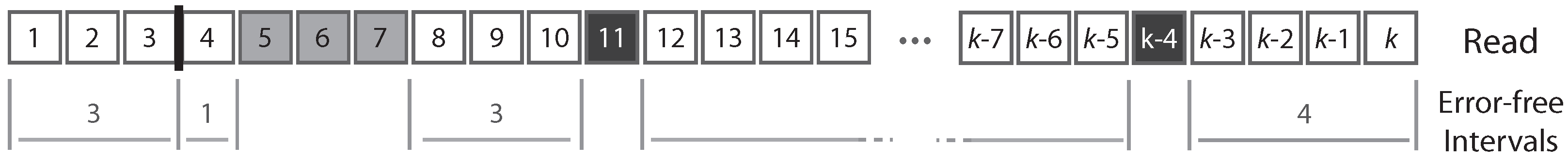
4.1. Reads, Error Symbols and Error-Free Intervals

From the experimental point of view, a sequencing read is the result of an assay on some polymer of nucleic acid. The output of the assay is the decoded sequence of monomers that compose the molecule. Three types of sequencing errors can occur: substitutions, deletions and insertions. A substitution is a nucleotide that is different in the molecule and in the read, a deletion is a nucleotide that is present in the molecule but not in the read, and an insertion is a nucleotide that is absent in the molecule but present in the read. For our purpose, the focus is not the nucleotide sequence per se, but whether the nucleotides are correct. Thus, we need only four symbols to describe a read: one for each type of error, plus one for correct nucleotides. In this view, a read is a finite sequence of letters from an alphabet of four symbols. Figure 1 shows the typical structure of a read.
A read can be partitioned uniquely into maximal sequences of identical symbols referred to as “intervals”. Thus, reads can also be seen as sequences of either error-free intervals or error symbols (Figure 2). As detailed below, this will allow us to control the size of the largest error-free interval.
These concepts established, we can compute seeding probabilities in the read mapping problem. We define an “exact γ -seed”, or simply a seed, as an exact match of minimum size γ between the read and the actual sequence of the molecule. In other words, an exact γ -seed is an error-free interval of size at least γ . Because of sequencing errors, it could be that the read contains no seed. In this case, the read cannot be mapped to the correct location if the mapping algorithm requires seeds of size γ or greater.
Our goal is to construct estimators of the probability that a read contains an exact γ -seed based on expected sequencing errors. For this, we will construct the weighted generating functions of reads that do not contain an exact γ -seed by decomposing them as sequences of either error symbols or error-free intervals of size less than γ . We will obtain their weighted generating functions from Theorem 1 and use Theorem 2 to approximate their probability of occurrence. With the weighted generating function of all the reads R ( z ) , and that of reads without an exact γ -seed S γ ( z ) , the probability that a read of size k has no exact γ -seed can be computed as [ z k ] S γ ( z ) / [ z k ] R ( z ) , i.e., the total weight of reads of size k without seed divided by the total weight of reads of size k.

4.2. Substitutions Only

In the simplest model, we assume that errors can be only substitutions, and that they occur with the same probability p for every nucleotide. Importantly, the model is not overly simple and it has some real applications. For instance, it describes reasonably well the error model of the Illumina platforms, where p is around 0.01 [26].
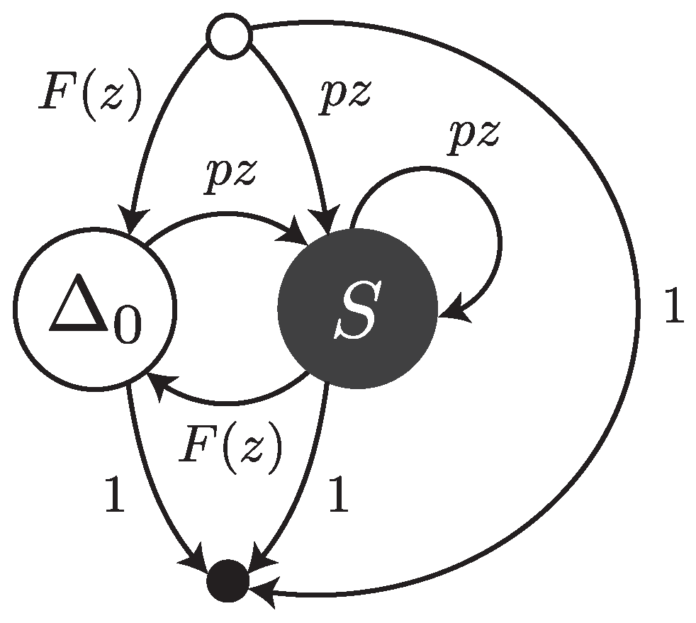
Under this error model, reads are sequences of single substitutions or error-free intervals. They can be thought of as walks on the transfer graph shown in Figure 3. The symbol Δ 0 stands for an error-free interval and the symbol S stands for a single substitution. F ( z ) and p z are the weighted generating functions of error-free intervals and substitutions, respectively. The fact that an error-free interval cannot follow another error-free interval is a consequence of the definition: two consecutive intervals are automatically merged into a single one.
A substitution is a single nucleotide and thus has size 1. Because substitutions have probability p, their weighted generating function is p z . Conversely, the weighted generating function of correct nucleotides is q z , where q = 1 p . Error-free intervals are non-empty sequences of correct nucleotides, so by Proposition 1 their weighted generating function is
F ( z ) = q z + ( q z ) 2 + ( q z ) 3 + = q z 1 q z .
The transfer matrix of the graph shown in Figure 3 is
M ( z ) =     Δ 0     S   Δ 0 S ( 0 F ( z ) p z 1 0 0 p z 1 0 F ( z ) p z 1 0 0 0 0 ) .
With the notations of Theorem 1, we have H ( z ) = ( F ( z ) , p z ) , T ( z ) = ( 1 , 1 ) , ψ ( z ) = 1 and
M ( z ) = Δ 0     S Δ 0 S ( 0 p z F ( z ) p z ) .
Applying Theorem 1, R ( z ) , the weighted generating function of all reads is found from the formula R ( z ) = ψ ( z ) + H ( z ) · ( I M ( z ) ) 1 · T ( z ) , which, in this case, translates to
R ( z ) = 1 + ( F ( z ) , p z ) · 1 λ ( z ) 1 p z p z F ( z ) 1 · 1 1 ,
where λ ( z ) = 1 p z ( 1 + F ( z ) ) is the determinant of I M ( z ) . Using equation (8), this expression simplifies to
R ( z ) = 1 + F ( z ) 1 p z ( 1 + F ( z ) ) = 1 1 z .
Since 1 / ( 1 z ) = 1 + z + z 2 + , the total weight of reads of size k is equal to 1 for any k 0 . As a consequence, [ z k ] R ( z ) = 1 and the probability that a read of size k has no exact γ -seed is equal to [ z k ] S γ ( z ) . To find the weighted generating function of reads without an exact γ -seed, we limit error-free intervals to a maximum size of γ 1 . To do this, we can replace F ( z ) in expression (9) by its truncation F γ ( z ) = q z + ( q z ) 2 + + ( q z ) γ 1 . We obtain
S γ ( z ) = 1 + F γ ( z ) 1 p z 1 + F γ ( z ) = 1 + q z + + ( q z ) γ 1 1 p z 1 + q z + + ( q z ) γ 1 .
Now applying Theorem 2 to the expression of S γ ( z ) above, we obtain the following proposition.
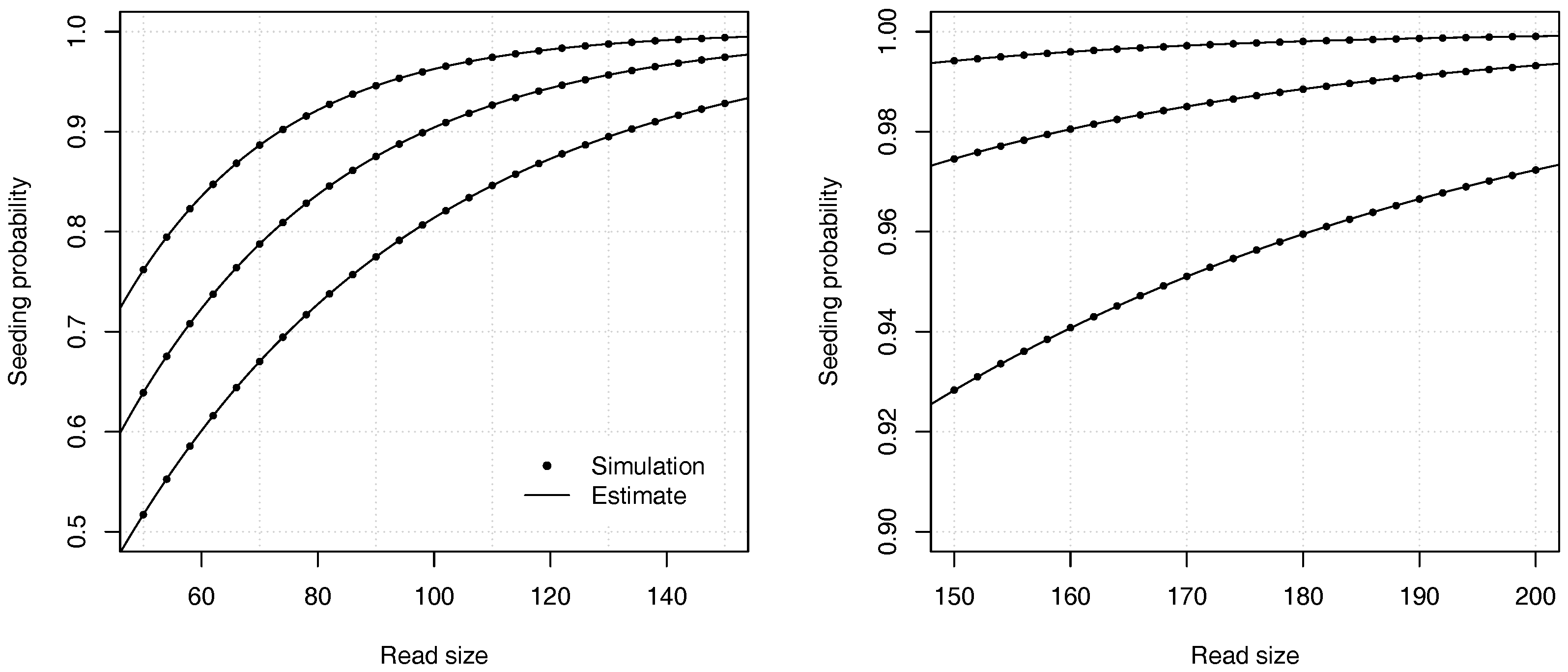
Proposition 2.
The probability that a read of size k has no seed under the uniform substitutions model is asymptotically equivalent to
C z 1 k + 1 ,
where z 1 is the root with smallest modulus of 1 p z ( 1 + q z + + ( q z ) γ 1 ) , and where
C = ( 1 q z 1 ) 2 p 2 z 1 1 ( γ + 1 γ q z 1 ) ( q z 1 ) γ .
If z 1 = 1 / q , expression (11) is undefined and the constant C should be computed as P ( z 1 ) / Q ( z 1 ) , where P ( z ) and Q ( z ) are the respective numerator and denominator of S γ ( z ) in expression (10).
Example 3.
Approximate the probability that a read of size k = 100 has no seed for γ = 17 and for a substitution rate p = 0.1 . To find the dominant singularity of S 17 , we solve 1 0.1 z × ( 1 + 0.9 z + + ( 0.9 z ) 16 ) = 0 . We rewrite the equation as 1 0.1 z × ( 1 ( 0.9 z ) 17 ) / ( 1 0.9 z ) = 0 and use numerical bisection to obtain z 1 1.0268856 . Substituting this value in equation (11) yields C 1.396145 , so the probability that a read contains no seed is approximately 1.396145 / 1.0268856 101 0.095763 . For comparison, a 99% confidence interval obtained by performing 10 billion random simulations is 0.09575 0.09577 . The computational cost of the analytic combinatorics approach is infinitesimal compared to the random simulations, and the precision is much higher for k = 100 .
Overall, the analytic combinatorics estimates are accurate. Figure 4 illustrates the precision of the estimates for different values of the error rate p and of the read size k.
One can also compute the probabilities by recurrence using Theorem 3, after replacing the term 1 + q z + + ( q z ) γ 1 by ( 1 ( q z ) γ ) / ( 1 q z ) in expression (10). Denoting [ z k ] S γ ( z ) as s k , one obtains for every positive integer γ
s k = 1 , if   0 k < γ , 1 q γ , if   k = γ , s k 1 p q γ · s k γ 1 , if   k > γ .

4.3. Substitutions and Deletions

We now consider a model where errors can be deletions or substitutions, but not insertions. This case is not very realistic, but it will be useful to clarify how to construct reads with potential deletions. As in the case of uniform substitutions, we assume that every nucleotide call is false with a probability p and true with a probability 1 p = q . Here, we also assume that between every pair of decoded nucleotides in the read, an arbitrary number of nucleotides from the original molecule are deleted with probability δ . Regardless of the number of deleted nucleotides, all the deletions are equivalent when the read is viewed as a sequence of error-free intervals or error symbols (see Figure 2).
A deletion may be adjacent to a substitution, or lie between two correct nucleotides. In the first case, the deletion does not interrupt any error-free interval so it does not change the probability that the read contains a seed. For this reason, we ignore deletions next to substitutions. More precisely, we assume that they can occur, but whether they do has no importance for the problem.
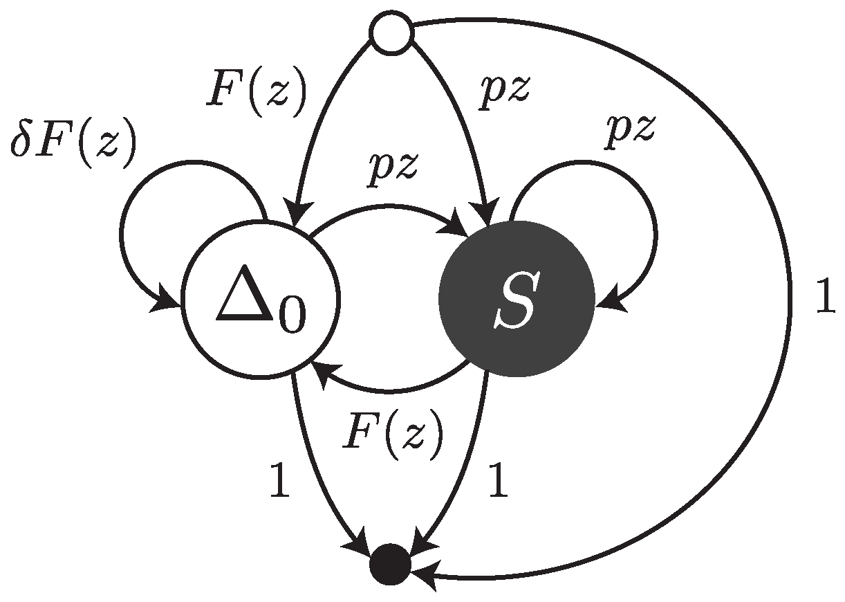
Under this error model, a read can be thought of as a walk on the transfer graph shown in Figure 5. The graph is almost the same as the one shown Figure 3; the only difference is the edge labelled δ F ( z ) from Δ 0 to Δ 0 . This edge represents the fact that an error-free interval can follow another one if a deletion with weighted generating function δ is present in between (as illustrated for instance in Figure 2).
The weighted generating function of error-free intervals F ( z ) has a different expression from that of Section 4.2. When the size of an error-free interval is 1, the weighted generating function is just q z . For a size k > 1 , there are k 1 “spaces” between the nucleotides, so the weighted generating function is ( 1 δ ) k 1 ( q z ) k . Summing for all the possible sizes, we obtain the weighted generating function of error-free intervals as
F ( z ) = q z + ( 1 δ ) ( q z ) 2 + ( 1 δ ) 2 ( q z ) 3 + = q z 1 ( 1 δ ) q z .
The transfer matrix of the graph shown in Figure 5 is
M ( z ) =     Δ 0     S   Δ 0 S ( 0 F ( z ) p z 1 0 δ F ( z ) p z 1 0 F ( z ) p z 1 0 0 0 0 ) .
With the notations of Theorem 1, H ( z ) = ( F ( z ) , p z ) , T ( z ) = ( 1 , 1 ) , ψ ( z ) = 1 and
M ( z ) =     Δ 0 S Δ 0 S ( δ F ( z ) p z F ( z ) p z ) .
From Theorem 1, the weighted generating function of all reads is
R ( z ) = 1 + ( F ( z ) , p z ) · 1 λ ( z ) 1 p z p z F ( z ) 1 δ F ( z ) · 1 1 ,
where λ ( z ) = 1 p z ( p z ( 1 δ ) + δ ) F ( z ) is the determinant of I M ( z ) . Using equation (13), this expression simplifies to
R ( z ) = 1 + ( 1 δ ) F ( z ) 1 p z p z ( 1 δ ) + δ F ( z ) = 1 1 z .
As in Section 4.2, the result is 1 / ( 1 z ) = 1 + z + z 2 + , which means that the probability that a read of size k contains no seed is equal to [ z k ] S γ ( z ) . To find the weighted generating function of reads without an exact γ -seed, we bound the size of error-free intervals to a maximum of γ 1 , i.e., we replace F ( z ) by its truncation F γ ( z ) = q z + ( 1 δ ) ( q z ) 2 + + ( 1 δ ) γ 2 ( q z ) γ 1 . With this, the weighted generating function of reads without seed is
S γ ( z ) = 1 + ( 1 δ ) F γ ( z ) 1 p z p z ( 1 δ ) + δ F γ ( z ) .
Applying Theorem 2 to this expression, we obtain the following proposition.
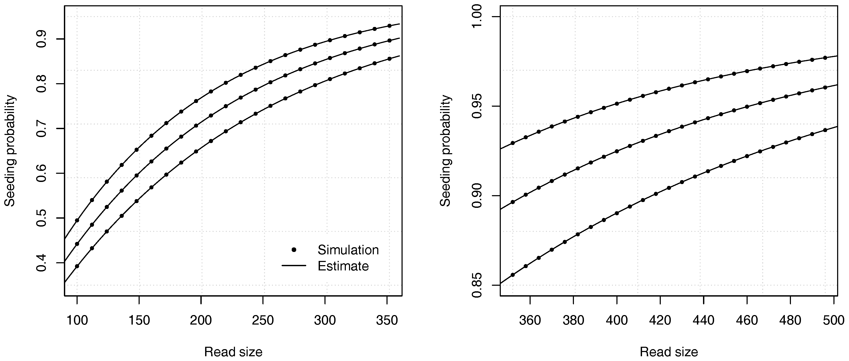
Proposition 3.
The probability that a read of size k has no seed under the model of uniform substitutions and deletions is asymptotically equivalent to
C z 1 k + 1 ,
where z 1 is the root with smallest modulus of 1 p z p z ( 1 δ ) + δ ( q z + ( 1 δ ) ( q z ) 2 + + ( 1 δ ) γ 2 ( q z ) γ 1 ) , and where
C = z 1 1 ( 1 δ ) q z 1 2 ( p + q δ ) z 1 c 1 ( 1 δ ) γ 1 ( q z 1 ) γ δ + ( 1 δ ) p z 1 , w i t h c 1 = γ δ ( 1 δ ) ( γ 1 ) δ p ( ( γ 1 ) δ + γ + 1 ) z 1 γ ( 1 δ ) 2 p q z 1 2 .
If z 1 = 1 / ( ( 1 δ ) q ) , expression (16) is undefined and the constant C should be computed as P ( z 1 ) / Q ( z 1 ) , where P ( z ) and Q ( z ) are the respective numerator and denominator of S γ ( z ) in expression (15).
Example 4.
Approximate the probability that a read of size k = 100 has no seed for γ = 17 , p = 0.05 and δ = 0.15 . To find the dominant singularity of S 17 , we solve 1 0.05 z 0.0425 z + 0.15 0.95 z + 0.85 ( 0.95 z ) 2 + + 0.85 15 ( 0.95 z ) 16 = 0 . We write it as 1 0.05 z ( 0.0425 z + 0.15 ) ( 0.95 z 0.85 16 ( 0.95 z ) 17 ) / ( 1 0.8075 z ) = 0 and use numerical bisection to obtain z 1 1.006705 . Now, substituting the obtained value in Equation (16) gives C 1.096177 , so the probability is approximately 1.096177 / 1.006705 101 0.558141 . For comparison, a 99% confidence interval obtained by performing 10 billion random simulations is 0.55813 0.55816 .
Once again, the analytic combinatorics estimates are accurate. Figure 6 illustrates the precision of the estimates for different values of the deletion rate δ and of the read size k.
The probabilities can also be computed by recurrence using Theorem 3, after replacing F γ ( z ) by q z ( 1 ( ( 1 δ ) q z ) γ 1 ) / ( 1 ( 1 δ ) q z ) in expression (15). Denoting [ z k ] S γ ( z ) as s k , one obtains for every integer γ > 1
s k = 1 , if   0 k < γ , 1 ( 1 δ ) γ 1 q γ , if   k = γ , s k 1 δ q γ ( 1 δ ) γ 1 · s k γ p q γ ( 1 δ ) γ · s k γ 1 , if   k > γ .

4.4. Substitutions, Deletions and Insertions

Here, we consider a model where all types of errors are allowed (also referred to as the “full error model”). Introducing insertions brings two additional difficulties: the first is that a substitution is indistinguishable from an insertion followed by a deletion (or a deletion followed by an insertion). By convention, we will count all these cases as substitutions. As a consequence, a deletion can never be found next to an insertion. The second difficulty is that insertions usually come in bursts. This is also the case of deletions, but we could neglect it because this does not affect the size of the interval (all deletions have size 0).
To model insertion bursts, we need to assign a probability r to the first insertion, and a probability r ˜ > r to all subsequent insertions of the burst. We will still denote the probability of a substitution p and that of a correct nucleotide q, but here p + q + r = 1 . We will also assume that an insertion burst stops with probability 1 r ˜ at each position of the burst.
Under this error model, reads can be thought of as walks on the transfer graph shown in Figure 7. To not overload the figure, the body of the transfer graph is represented on the left, and the head and tail vertices on the right. The symbols Δ 0 , S and I stand for error-free intervals, single substitutions and single insertions, respectively. The terms F ( z ) , p z and δ F ( z ) are the same as in Section 4.3. The terms r z and r ˜ z are the weighted generating functions of the first inserted nucleotide and of all subsequent nucleotides of the insertion burst, respectively. The burst terminates with probability 1 r ˜ and is followed by an error-free interval or by a substitution. The total weight of these two cases is p + q < 1 , so we need to further scale the weighted generating functions by a factor p + q = 1 r .
The expression of the weighted generating function of error-free intervals F ( z ) is the same as in Section 4.3, namely
F ( z ) = q z + ( 1 δ ) ( q z ) 2 + ( 1 δ ) 2 ( q z ) 3 + = q z 1 ( 1 δ ) q z .
The transfer matrix of the graph shown in Figure 7 is
M ( z ) =       Δ 0         S   I   Δ 0 S I ( 0 F ( z ) p z r z 1 0 δ F ( z ) p z r z 1 0 F ( z ) p z r z 1 0 1 r ˜ 1 r F ( z ) 1 r ˜ 1 r p z r ˜ z 1 0 0 0 0 0 ) .
With the notations of Theorem 1, H ( z ) = ( F ( z ) , p z , r z ) , T ( z ) = ( 1 , 1 , 1 ) , ψ ( z ) = 1 and
M ( z ) =   Δ 0     S           I Δ 0 S I ( δ F ( z ) p z r z F ( z ) p z r z 1 r ˜ 1 r F ( z ) 1 r ˜ 1 r p z r ˜ z ) .
From Theorem 1, the weighted generating function of all reads is ψ ( z ) + H ( z ) · ( I M ( z ) ) 1 · T ( z ) , which is equal to
R ( z ) = ( 1 r ) 1 ( r ˜ r ) z 1 + ( 1 δ ) F ( z ) 1 a ( z ) b ( z ) F ( z ) ,
where a ( z ) and b ( z ) are second degree polynomials defined as
a ( z ) = r + ( 1 r ) ( p + r ˜ ) z p ( r ˜ r ) z 2 , and b ( z ) = δ ( 1 r ) + ( 1 r ) ( p δ ( p + r ˜ ) ) + ( 1 r ˜ ) r z p ( 1 δ ) ( r ˜ r ) z 2 .
Substituting in (18) the expressions of F ( z ) , a ( z ) and b ( z ) , we find
R ( z ) = 1 1 z .
Again, we obtain the simple expression 1 / ( 1 z ) = 1 + z + z 2 + and the probability that a read of size k contains no seed is [ z k ] S γ ( z ) . To find the weighted generating function of reads without an exact γ -seed, we replace F ( z ) in expression (18) by its truncated version
F γ ( z ) = q z + ( 1 δ ) ( q z ) 2 + ( 1 δ ) 2 ( q z ) 3 + + ( 1 δ ) γ 2 ( q z ) γ 1 .
We obtain the following expression
S γ ( z ) = ( 1 r ) 1 ( r ˜ r ) z 1 + ( 1 δ ) F γ ( z ) 1 a ( z ) b ( z ) F γ ( z ) ,
where a ( z ) and b ( z ) are defined as in expression (19).
Remark 2.
Note that when r = r ˜ = 0 , then a ( z ) = p z and b ( z ) = p z ( 1 δ ) + δ , expression (21) becomes
S γ ( z ) = 1 + ( 1 δ ) F γ ( z ) 1 p z ( p z ( 1 δ ) + δ ) ) F γ ( z ) .
This is expression (15), i.e., the model described in Section 4.3. When we also have δ = 0 , this expression further simplifies to
S γ ( z ) = 1 + F γ ( z ) 1 p z ( 1 + F γ ( z ) ) .
This is expression (10), i.e., the model described in Section 4.2. In other words, the error models described previously are special cases of this error model.
As in the previous sections, we can use Theorem 2 to obtain asymptotic approximations for the probability that the reads contain no seed.
Proposition 4.
The probability that a read of size k has no seed under the error model with substitutions, deletions and insertions is asymptotically equivalent to
C z 1 k + 1 ,
where z 1 is the root with smallest modulus of the polynomial 1 a ( z ) b ( z ) F γ ( z ) and
C = ( 1 r ) 1 ( r ˜ r ) z 1 1 + ( 1 δ ) F γ ( z 1 ) a ( z 1 ) + b ( z 1 ) F γ ( z 1 ) + b ( z 1 ) F γ ( z 1 ) .
If z 1 = 1 / ( ( 1 δ ) q ) , then F γ ( z 1 ) = ( γ 1 ) / ( 1 δ ) and F γ ( z 1 ) = q γ ( γ 1 ) / 2 . Otherwise,
F γ ( z 1 ) = q z 1 1 ( 1 δ ) q z 1 γ 1 1 ( 1 δ ) q z 1 , a n d F γ ( z 1 ) = q 1 + ( 1 δ ) ( γ 1 ) q z 1 γ ( 1 δ ) q z 1 γ 1 1 ( 1 δ ) q z 1 2 .
If z 1 = 1 / ( r ˜ r ) , then 1 ( r ˜ r ) z divides the numerator and the denominator, which should be simplified to remain coprime. In this case, Theorem 2 should be applied to the simplified rational function.
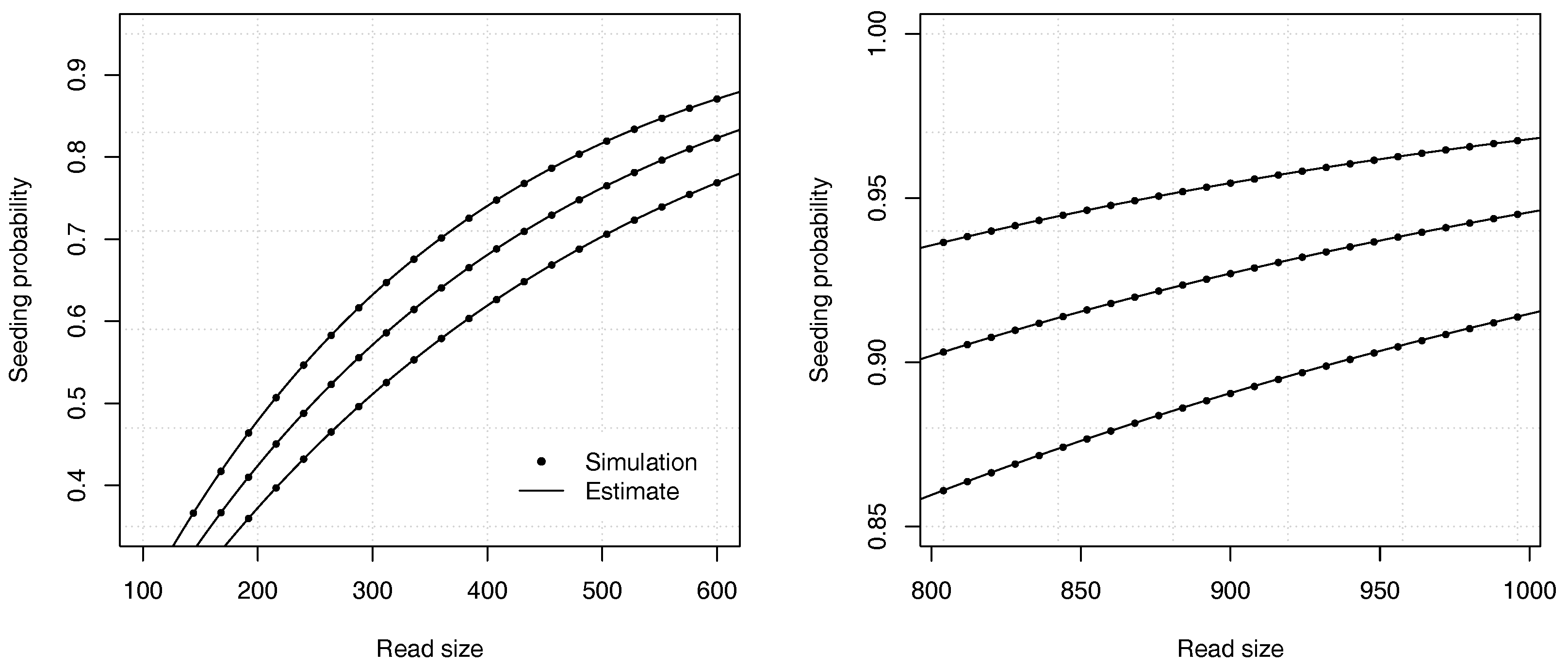
Example 5.
Approximate the probability that a read of size k = 100 has no seed for γ = 17 , p = 0.05 , δ = 0.15 , r = 0.05 and r ˜ = 0.45 . With these values, a ( z ) = 0.05 + 0.475 z 0.02 z 2 and b ( z ) = 0.1425 + 0.00375 z 0.017 z 2 . We need to solve 0.95 0.475 z + 0.02 z 2 ( 0.1425 + 0.00375 z 0.017 z 2 ) ( 0.9 z + 0.85 ( 0.9 z ) 2 + + 0.85 15 ( 0.9 z ) 16 ) = 0 . We rewrite the equation as 0.95 0.475 z + 0.02 z 2 ( 0.1425 + 0.00375 z 0.017 z 2 ) ( 0.9 z 0.85 15 ( 0.9 z ) 16 ) / ( 1 0.765 z ) = 0 and use bisection to solve it numerically, yielding z 1 1.00295617 . From expression (22), we obtain C 1.042504 , so the probability that a read contains no seed is approximately 1.042504 / 1 . 00295617 101 0.773749 . For comparison, a 99% confidence interval obtained by performing 10 billion random simulations is 0.77373 0.77376 .
Once again, the analytic combinatorics estimates are accurate. Figure 8 illustrates the precision of the estimates for different values of the insertion rate r and of the read size k.
The probabilities can also be computed by recurrence using Theorem 3, after replacing F γ ( z ) by q z ( 1 ( ( 1 δ ) q z ) γ 1 ) / ( 1 ( 1 δ ) q z ) in expression (21). Denoting [ z k ] S γ ( z ) as s k , one obtains for every integer γ > 2
s k = 1 if   0 k < γ , 1 ( 1 δ ) γ 1 q γ if   k = γ , 1 ( 1 δ ) γ 1 q γ 1 r r ˜ 1 r + p + q δ if   k = γ + 1 , ( 1 + r ˜ r ) · s k 1 ( r ˜ r ) · s k 2 δ q γ ( 1 δ ) γ 1 · s k γ if   k > γ + 1 . + q γ ( 1 δ ) γ 1 δ ( p + r ˜ ) p r 1 r ˜ 1 r · s k γ 1 + p q γ ( 1 δ ) γ r ˜ r 1 r · s k γ 2

4.5. Accuracy of the Approximations

So far, all the examples showed that the analytic combinatorics approximations are accurate. Indeed, the main motivation for our approach is to find estimates that converge exponentially fast to the target value. To find out whether we can use the approximations in place of the true values, we need to describe the behavior of the estimates in the worst conditions. The approximations become more accurate as the size of the sequence increases, i.e., as the reads become longer. This is somewhat inconvenient: the read size is usually fixed by the technology or by the problem at hand, so the user does not have easy ways to improve the accuracy. Overall, the approximations described above tend to be less accurate for short reads.
Another aspect is convergence speed. The proof of Theorem 2 shows that the rate of convergence is fastest when the dominant singularity has a significantly smaller modulus than the other singularities. Conversely, convergence is slowest when at least one other singularity is almost as close to 0. The worst case for the approximation is thus when the reads are small and when the parameters are such that singularities have relatively close moduli. It can be shown that, for the error model of uniform substitutions, this corresponds to small values of the error rate p (see Appendix A).
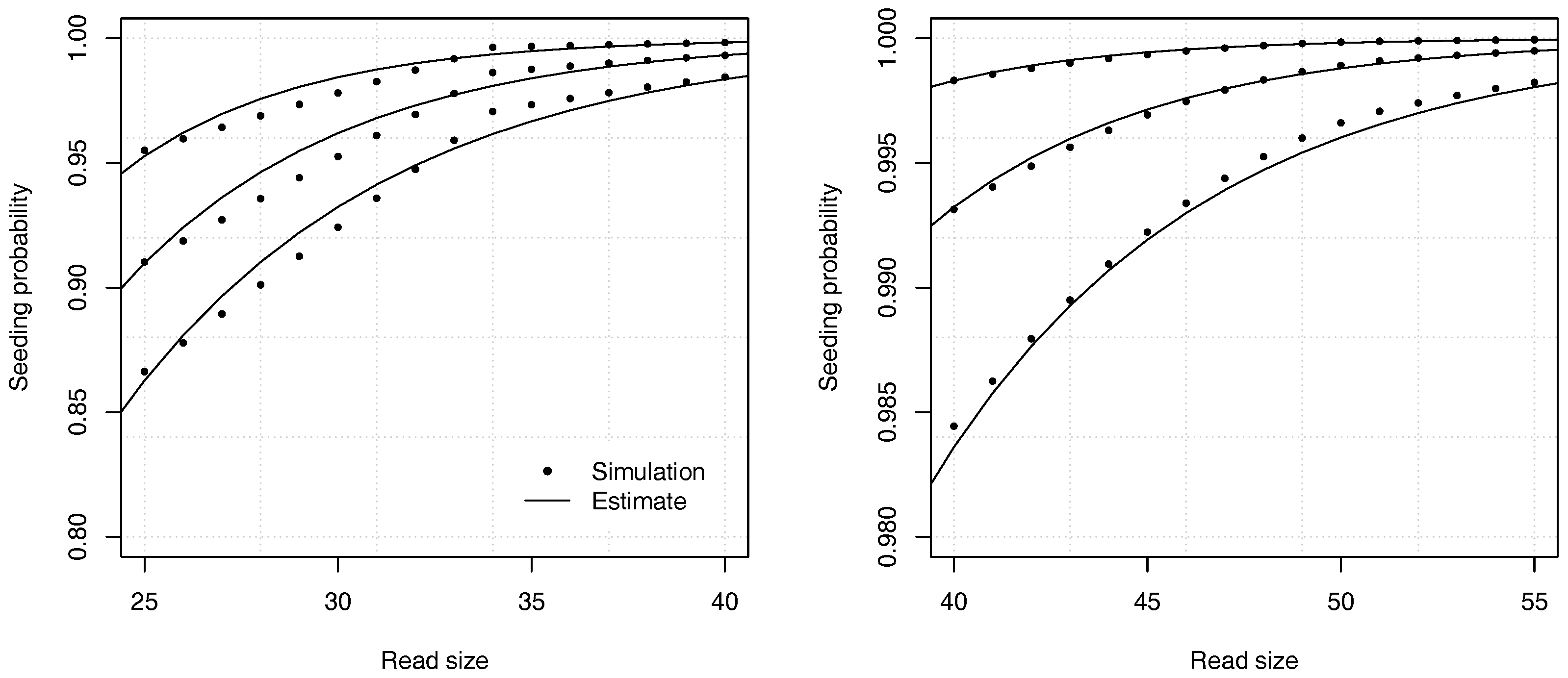
In practical terms, the situation above describes the specifications of the Illumina technology, where errors are almost always substitutions, occurring at a frequency around 1% on current instruments. Since the reads are often around 50 nucleotides, the analytic combinatorics estimates of the seeding probabilities are typically less accurate than suggested in the previous sections.
Figure 9 shows the accuracy of the estimates in one of the worst cases. The analytic combinatorics estimates are clearly distinct from the simulation estimates at the chosen scale, but the absolute difference is never higher than approximately 0.015 (and lower for read sizes above 40). Whether this error is acceptable depends on the problem. Often p itself must be estimated, which is a more serious limitation on the precision than the convergence speed of the estimates. In most practical applications, the approximation error of Theorem 2 can be tolerated even in the worst case, but it is important to bear in mind that it may not be negligible for reads of size 50 or lower. If this level of precision is insufficient, the best option is to compute the coefficients by recurrence.
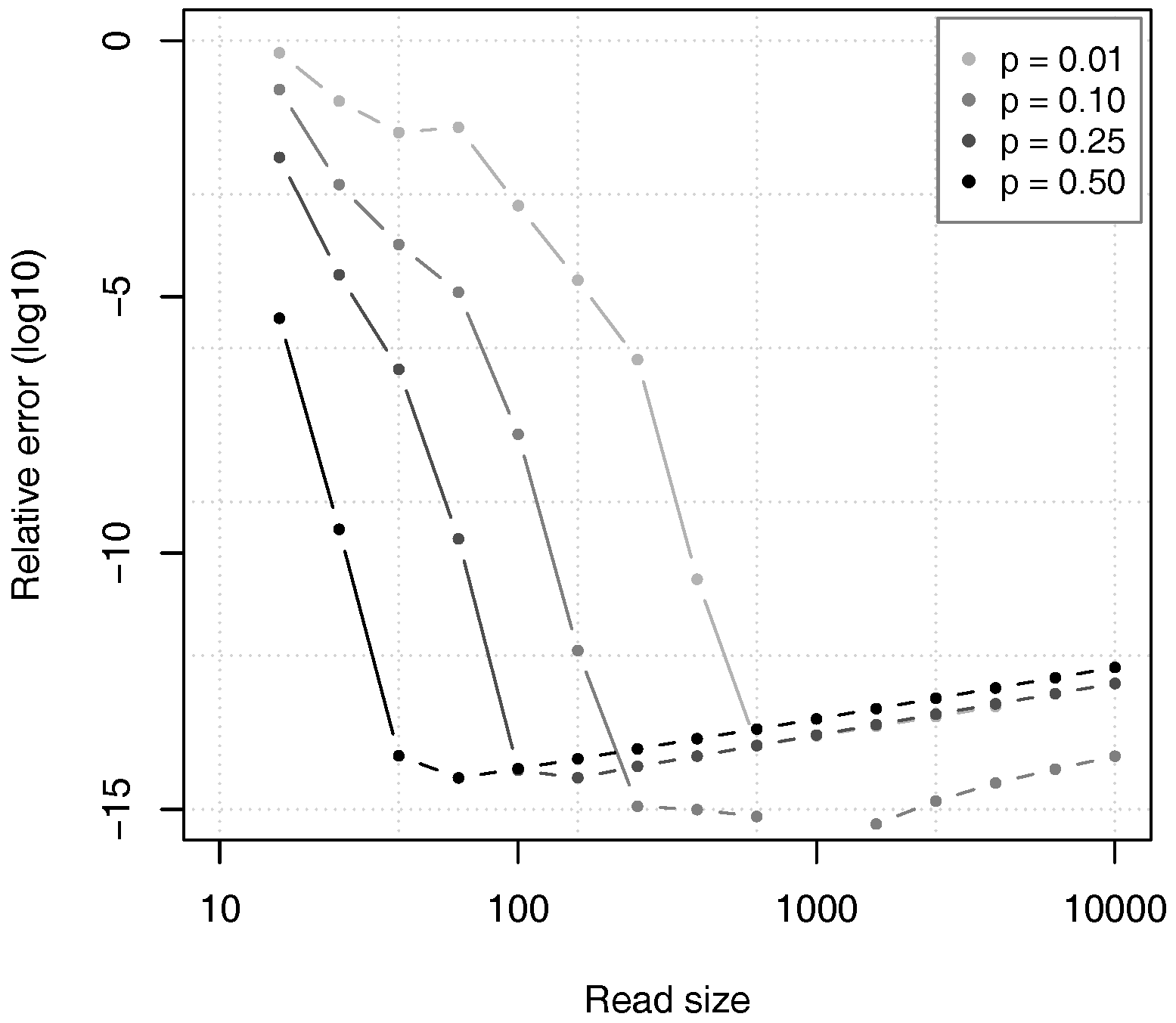
For long reads, the approximations rapidly gain in accuracy. Importantly, the calculations are also numerically stable, even for very long reads and for very high values of the error rate. To explore the behavior of the estimates, they were computed over a wide range of conditions, and compared to the values obtained by computing recurrence (12).
The value of s k is the exact probability that a read of size k does not contain a seed in the uniform substitution error model, when the probability of substitution is equal to p. However, because the numbers are represented with finite precision, the computed value of s k is also inexact in practice. Figure 10 shows the relative error of the estimates given by Proposition 2, as compared to the value of s k computed through equation (12) in double precision arithmetic. For all the tested values of p, the relative error first decreases to approximately 10 15 and then slowly rises. The reason is that the theoretical accuracy of the estimates increases with the read size k, as justified by Theorem 2, but the errors in numerical approximations also increase and they finally dominate the error.
In spite of this artefact, it is clear that the relative error of the estimates remains low for very large read sizes. This means that the estimates are sufficiently close to the exact value, and that the calculations are numerically stable. Figure 10 also confirms that the value of p has a large influence on the convergence speed of the approximation. For high values of p, the relative error drops faster than for low values of p, as argued above.
The main reason for the numerical stability of the estimates is that the polynomial equations to solve can be properly represented with double precision numbers. For instance, in the extreme case of seeds of size 30 with a substitution rate p = 0.5 , the leading term of Q ( z ) in Proposition 2 is p ( 1 p ) 29 z 30 10 9 z 30 . This is several orders of magnitude above the machine epsilon (approximately equal to 2.2 × 10 16 on most computers), sufficient to guarantee that this term will not underflow during the calculations, and thus that the dominant singularity will be computed with an adequate precision. The same applies for the other error models, as long as the rate of sequencing errors remains above 0.5 , which is the case in the vast majority of practical applications.
In summary, the estimates presented above are accurate and numerically stable. In the case of short reads with low error rate, the precision may be limiting for some applications, but the approximations can be replaced by exact solutions. The approach presented here is thus a practical solution for computing seeding probabilities.

5. Discussion

In this article, we exposed the analytic combinatorics approach to compute seeding probabilities in the read mapping problem. The general strategy of analytic combinatorics is to define combinatorial “atoms” with simple weighted generating functions (e.g., nucleotide symbols), combine these atoms into objects of increasing complexity (e.g., error-free intervals or reads without seed), construct their weighted generating functions from simple rules (e.g., through Theorem 1), and finally analyze the singularities of the weighted generating functions to approximate the quantities of interest (e.g., through Theorem 2). We can also use the generating function to set up an exact recurrence to find those quantities.
The seeding probabilities derived here are robust and relatively straightforward, as they only entail solving a polynomial equation in real space. For short reads, where the precision of the approximations may be an issue, the solution is better computed by recurrence. Mapping high throughput sequencing reads generates a sufficient amount of data to estimate the parameters of the error model. One can thus envision auto-tuning the seeding heuristic of read mapping during the run. This can give tight and automatic control over the seeding probability. Alternatively, the theory developed above could be used to help users choose the parameter values of the mapping algorithm.
Seeding is not only used in mapping, but also in other alignment problems. In this regard, the work presented above can be applied to different contexts. That said, mapping high throughput sequencing reads is a “sweet spot” for analytic combinatorics because the sequences are usually long enough for the approximations to be accurate.
In summary, analytic combinatorics is a powerful strategy that comes with a rich toolbox that has many applications in modern bioinformatics. More applications will see the light when this theory is more widely known in the bioinformaics community.

Acknowledgments

I would like to thank the anonymous reviewers for their important contributions to this work. I would also like to thank Eduard Valera Zorita, Patrick Berger and Roman Cheplyaka for their comments on this work. I acknowledge the financial support of the Spanish Ministry of Economy and Competitiveness (‘Centro de Excelencia Severo Ochoa 2013-2017’, Plan Nacional BFU2012-37168), of the CERCA (Centres de Recerca de Catalunya) Programme / Generalitat de Catalunya, and of the European Research Council (Synergy Grant 609989).

Conflicts of Interest

The author declares no conflict of interest.

Appendix A

Here, we show that in the error model of Section 4.2, the moduli of the singularities of S γ ( z ) expressed in (10) get closer to each other as p decreases. More specifically, | z j | | z m | ( p 0 ) for any two singularities z j and z m .
Recall that the singularities of S γ ( z ) are the roots of Q ( z ) = 1 p z 1 + q z + + ( q z ) γ 1 , where q = 1 p . Let z j be a root of Q and rearrange the terms of the equation Q ( z j ) = 0 to obtain z j 1 + q z j + + ( q z j ) γ 1 = 1 / p . As p 0 , the right-hand side tends to + so the left-hand side must also tend to + , imposing lim p 0 | z j | = + .
Multiply Q ( z ) = 0 by ( 1 q z ) and use 1 + q z + + ( q z ) γ 1 = 1 ( q z ) γ / ( 1 q z ) , where z 1 / q to see that every singularity z j solves the equation ( 1 q z ) Q ( z ) = 1 z + p q γ z γ + 1 = 0 or equivalently
1 1 / z j = p q γ z j γ , z j 1 q .
Since lim p 0 | z j | = + , taking the limit of the equation above yields
lim p 0 q p 1 / γ z j γ = 1 , i . e . , | z j | 1 q p 1 / γ ( p 0 ) .
This is sufficient to prove that | z j | | z m | ( p 0 ) for any two singularities z j and z m , but we can further show that
z j e 2 i ( j 1 ) π / γ q p 1 / γ ( p 0 ) , j = 1 , 2 , , γ .
From (A1), we see that the terms q p 1 / γ z j tend to γ -th roots of unity, which have γ possible values. If we prove that Q has γ distinct roots, then each of them must correspond to a different γ -th root of unity and (A2) will follow. Since Q is a polynomial of degree γ , we must prove that all its roots have multiplicity 1, i.e., that they do not solve Q ( z ) = 0 .
Let V ( z ) = ( 1 q z ) Q ( z ) = 1 z + p q γ z γ + 1 , so V ( z ) = 1 + ( γ + 1 ) p q γ z γ , and compute the greatest common divisor of V ( z ) and V ( z ) :
gcd V ( z ) , V ( z ) = gcd ( V ( z ) z γ + 1 V ( z ) , V ( z ) ) = gcd ( 1 γ z γ + 1 , V ( z ) ) .
Up to a constant factor independent of z, the greatest common divisor is either 1 or 1 γ z / ( γ + 1 ) . If z = 1 + 1 / γ is not a root of V ( z ) , then V ( z ) and V ( z ) are relatively prime, so V ( z ) does not have any double roots and neither does Q ( z ) .
If z = 1 + 1 / γ is a root of V ( z ) , then the greatest common divisor is 1 γ z / ( γ + 1 ) so z = 1 + 1 / γ is a root of V ( z ) with multiplicity 2. This case arises when p = 1 / ( γ + 1 ) , which implies that z = 1 + 1 / γ = 1 / q . In V ( z ) = ( 1 q z ) Q ( z ) , the factor 1 q z contributes one occurrence of the root, so Q ( z ) contributes the other occurrence and z = 1 + 1 / γ is thus a single root of Q ( z ) .

References

  1. Reuter, J.A.; Spacek, D.V.; Snyder, M.P. High-throughput sequencing technologies. Mol. Cell 2015, 58, 586–597. [Google Scholar] [CrossRef] [PubMed]
  2. Quilez, J.; Vidal, E.; Dily, F.L.; Serra, F.; Cuartero, Y.; Stadhouders, R.; Graf, T.; Marti-Renom, M.A.; Beato, M.; Filion, G. Parallel sequencing lives, or what makes large sequencing projects successful. Gigascience 2017, 6, 1–6. [Google Scholar] [CrossRef] [PubMed]
  3. Li, H.; Homer, N. A survey of sequence alignment algorithms for next-generation sequencing. Brief. Bioinform. 2010, 11, 473–483. [Google Scholar] [CrossRef] [PubMed]
  4. Durbin, R.; Eddy, S.R.; Krogh, A.; Mitchison, G. Biological Sequence Analysis: Probabilistic Models of Proteins and Nucleic Acids; Cambridge University Press: Cambridge, UK, 1998. [Google Scholar]
  5. Sun, Y.; Buhler, J. Choosing the best heuristic for seeded alignment of DNA sequences. BMC Bioinform. 2006, 7, 133. [Google Scholar] [CrossRef] [PubMed]
  6. Altschul, S.F.; Gish, W.; Miller, W.; Myers, E.W.; Lipman, D.J. Basic local alignment search tool. J. Mol. Biol. 1990, 215, 403–410. [Google Scholar] [CrossRef]
  7. Karlin, S.; Altschul, S.F. Applications and statistics for multiple high-scoring segments in molecular sequences. Proc. Natl. Acad. Sci. USA 1993, 90, 5873–5877. [Google Scholar] [CrossRef] [PubMed]
  8. Karlin, S.; Altschul, S.F. Methods for assessing the statistical significance of molecular sequence features by using general scoring schemes. Proc. Natl. Acad. Sci. USA 1990, 87, 2264–2268. [Google Scholar] [CrossRef] [PubMed]
  9. Ferragina, P.; Manzini, G. Opportunistic Data Structures with Applications. In Proceedings of the 41st Annual Symposium on Foundations of Computer Science, Redondo Beach, CA, USA, 12–14 November 2000; pp. 390–398. [Google Scholar]
  10. Li, H.; Durbin, R. Fast and accurate short read alignment with Burrows-Wheeler transform. Bioinformatics 2009, 25, 1754–1760. [Google Scholar] [CrossRef] [PubMed]
  11. Langmead, B.; Trapnell, C.; Pop, M.; Salzberg, S.L. Ultrafast and memory-efficient alignment of short DNA sequences to the human genome. Genome Biol. 2009, 10, R25. [Google Scholar] [CrossRef] [PubMed]
  12. Flajolet, P.; Odlyzko, A. Singularity analysis of generating functions. SIAM J. Discrete Math. 1990, 3, 216–240. [Google Scholar] [CrossRef]
  13. Flajolet, P.; Sedgewick, R. An introduction to the analysis of algorithms, 2nd ed.; Addison-Wesley Longman Publishing Co., Inc.: Boston, MA, USA, 1996. [Google Scholar]
  14. Flajolet, P.; Sedgewick, R. Analytic Combinatorics, 1st ed.; Cambridge University Press: New York, NY, USA, 2009. [Google Scholar]
  15. Lladser, M.E.; Betterton, M.D.; Knight, R. Multiple pattern matching: A Markov chain approach. J. Math. Biol. 2008, 56, 51–92. [Google Scholar] [CrossRef] [PubMed]
  16. Fu, J.C.; Koutras, M.V. Distribution Theory of Runs: A Markov Chain Approach. J. Am. Stat. Assoc. 1994, 89, 1050–1058. [Google Scholar] [CrossRef]
  17. Regnier, M.; Kirakossian, Z.; Furletova, E.; Roytberg, M. A word counting graph. In London Algorithmics 2008: Theory and Practice (Texts in Algorithmics); Chan, J., Daykin, J.W., Sohel, M., Eds.; Rahman London College Publications: London, UK, 2009; p. 31. [Google Scholar]
  18. Nuel, G. Pattern Markov Chains: Optimal Markov Chain Embedding Through Deterministic Finite Automata. J. Appl. Prob. 2008, 45, 226–243. [Google Scholar] [CrossRef]
  19. Nuel, G.; Delos, V. Counting Regular Expressions in Degenerated Sequences Through Lazy Markov Chain Embedding. In Forging Connections between Computational Mathematics and Computational Geometry: Papers from the 3rd International Conference on Computational Mathematics and Computational Geometry; Chen, K., Ravindran, A., Eds.; Springer International Publishing: Cham, Switzerland, 2016; pp. 235–246. [Google Scholar]
  20. Chaisson, M.J.; Tesler, G. Mapping single molecule sequencing reads using basic local alignment with successive refinement (BLASR): Application and theory. BMC Bioinform. 2012, 13, 238. [Google Scholar] [CrossRef] [PubMed]
  21. Joyal, A. Une théorie combinatoire des séries formelles. Adv. Math. 1981, 42, 1–82. [Google Scholar] [CrossRef]
  22. Bona, M. Handbook of Enumerative Combinatorics; CRC Press: Boca Raton, FL, USA, 2015. [Google Scholar]
  23. Flajolet, P.; Gardy, D.; Thimonier, L. Birthday Paradox, Coupon Collectors, Caching Algorithms and Self-organizing Search. Discrete Appl. Math. 1992, 39, 207–229. [Google Scholar] [CrossRef]
  24. Pemantle, R.; Wilson, M.C. Analytic Combinatorics in Several Variables; Cambridge University Press: New York, NY, USA, 2013. [Google Scholar]
  25. Bender, E.A. Asymptotic Methods in Enumeration. SIAM Rev. 1974, 16, 485–515. [Google Scholar] [CrossRef]
  26. Nakamura, K.; Oshima, T.; Morimoto, T.; Ikeda, S.; Yoshikawa, H.; Shiwa, Y.; Ishikawa, S.; Linak, M.C.; Hirai, A.; Takahashi, H.; et al. Sequence-specific error profile of Illumina sequencers. Nucleic Acids Res. 2011, 39, e90. [Google Scholar] [CrossRef] [PubMed]
  27. R Core Team. R: A Language and Environment for Statistical Computing; R Foundation for Statistical Computing: Vienna, Austria, 2015. [Google Scholar]
Figure 1. Read as sequence of symbols. Reads consist of correct nucleotides (white boxes), substitutions (black boxes), deletions (vertical bars) and insertions (grey boxes). A single deletion can correspond to several missing nucleotides.
Algorithms 11 00003 g001
Figure 2. Read as sequence of error-free intervals or error symbols. Consecutive correct nucleotides can be lumped together in error-free intervals. The representation of a read as a sequence of either error-free intervals or error symbols is unique.
Algorithms 11 00003 g002
Figure 3. Transfer graph of reads with uniform substitutions. Reads are viewed as sequences of error-free intervals (symbol Δ 0 ) or substitutions (symbol S). F ( z ) and p z are the weighted generating functions of error-free intervals and individual substitutions, respectively. The head vertex is represented as a small white circle, and the tail vertex as a small black circle.
Algorithms 11 00003 g003
Figure 4. Example estimates for substitutions only. The analytic combinatorics estimates of Proposition 2 are benchmarked against random simulations. Shown on both panels are the probabilities that a read of given size contains a seed, either estimated by 10,000,000 random simulations (dots), or by Proposition 2 (lines). The curves are drawn for γ = 17 and p = 0.08 , p = 0.10 or p = 0.12 (from top to bottom).
Algorithms 11 00003 g004
Figure 5. Transfer graph of reads with uniform substitutions and deletions. Reads are viewed as sequences of error-free intervals (symbol Δ 0 ) or substitutions (symbol S). Deletions are implicitly represented by the fact that an error-free interval can follow another one if a deletion is present in between. F ( z ) and p z are the weighted generating functions of error-free intervals and individual substitutions, respectively. δ F ( z ) is the weighted generating function of a deletion followed by an error-free interval. The head vertex is represented as a small white circle, and the tail vertex as a small black circle.
Algorithms 11 00003 g005
Figure 6. Example estimates for substitutions and deletions. The analytic combinatorics estimates of Proposition 3 are benchmarked against random simulations. Shown on both panels are the probabilities that a read of given size contains a seed, either estimated by 10,000,000 random simulations (dots), or by Proposition 3 (lines). The curves are drawn for γ = 17 , p = 0.05 and δ = 0.14 , δ = 0.15 or δ = 0.16 (from top to bottom).
Algorithms 11 00003 g006
Figure 7. Transfer graph of reads under the full error model. Reads are viewed as sequences of error-free intervals (symbol Δ 0 ), substitutions (symbol S) or insertions (symbol I). The body of the transfer graph is shown on the left, and the head and tail edges are shown on the right. F ( z ) and p z are the weighted generating functions of error-free intervals and individual substitutions, respectively. δ F ( z ) is the weighted generating function of a deletion followed by an error-free interval. r z and r ˜ z are the weighted generating functions of the first and all subsequent insertions of a burst, respectively. ( 1 r ˜ ) F ( z ) / ( 1 r ) is the weighted generating function of an error-free interval following an insertion and ( 1 r ˜ ) p z / ( 1 r ) is the weighted generating function of a substitutition following an insertion. The head vertex is represented as a small white circle, and the tail vertex as a small black circle.
Algorithms 11 00003 g007
Figure 8. Example estimates for substitutions, deletions and insertions. The analytic combinatorics estimates of Proposition 4 are benchmarked against random simulations. Shown on both panels are the probablities that a read of given size contains a seed, either estimated by 10,000,000 random simulations (dots), or by Proposition 4 (lines). The curves are drawn for γ = 17 , p = 0.05 , δ = 0.15 , r ˜ = 0.45 and r = 0.04 , r = 0.05 or r = 0.06 (from top to bottom).
Algorithms 11 00003 g008
Figure 9. Example worst case for seeding with substitutions only. The analytic combinatorics estimates of Proposition 2 are benchmarked against 10,000,000 random simulations. Shown on both panels are the probabilities that a read of given size contains a seed of size γ = 17 , either estimated by random simulations (dots), or by Proposition 2. The curves are drawn for p = 0.005 , p = 0.010 or p = 0.015 (from top to bottom). The largest difference between the estimates and the simulations is around 0.015 .
Algorithms 11 00003 g009
Figure 10. Accuracy of the approximations in the uniform substitution model. The estimates of Proposition 2 were computed for γ = 17 and different values of the substitution rate p ranging from 0.01 to 0.50 and for different read sizes k ranging from 15 to 10 , 000 . The reference target value was computed by recurrence through expression (12) and the relative error between the two terms was computed. All calculations were done in double precision arithmetic using R [27].
Algorithms 11 00003 g010

