Control-Oriented Models for SO Fuel Cells from the Angle of V&V: Analysis, Simplification Possibilities, Performance

Abstract

In this paper, we take a look at the analysis and parameter identification for control-oriented, dynamic models for the thermal subsystem of solid oxide fuel cells (SOFC) from the systematized point of view of verification and validation (V&V). First, we give a possible classification of models according to their verification degree which depends, for example, on the kind of arithmetic used for both formulation and simulation. Typical SOFC models, consisting of several coupled differential equations for gas preheaters and the temperature distribution in the stack module, do not have analytical solutions because of spatial nonlinearity. Therefore, in the next part of the paper, we describe in detail two possible ways to simplify such models so that the underlying differential equations can be solved analytically while still being sufficiently accurate to serve as the basis for control synthesis. The simplifying assumption is to approximate the heat capacities of the gases by zero-order polynomials (or first-oder polynomials, respectively) in the temperature. In the last, application-oriented part of the paper, we identify the parameters of these models as well as compare their performance and their ability to reflect the reality with the corresponding characteristics of models in which the heat capacities are represented by quadratic polynomials (the usual case). For this purpose, the framework UniVerMeC (Unified Framework for Verified GeoMetric Computations) is used, which allows us to employ different kinds of arithmetics including the interval one. This latter possibility ensures a high level of reliability of simulations and of the subsequent validation. Besides, it helps to take into account bounded uncertainty in measurements.

1. Introduction

Since 2010, the ongoing project VerIPC-SOFC has been dealing with modelling, simulation, and control of solid oxide fuel cell (SOFC) systems. During this time, highly efficient models for the thermal subsystem (consisting of the fuel cell stack and the anode and cathode gas preheaters) have been developed, verified, and validated on a test rig available at the Chair of Mechatronics at the University of Rostock [1,2]. The general goal of the project is to develop robust control methods that prevent over-temperatures in the stack by taking into account uncertainty in parameters, measurements and unknown influences on the system dynamics with the help of interval arithmetics. Our methods make use of sliding mode techniques [3,4] and of predictive control approaches [1].

Because both control techniques rely on dynamic system models given as ordinary differential equations (ODEs) in symbolic form, one of the important steps in the overall procedure is parameter optimisation. In this step, a least squares minimization problem is solved for systems of ODEs with a given structure (but usually without analytical solutions) against a large amount of data (several thousand measurements). In this paper, we bring structure into the modelling possibilities by using the so-called verification and validation analysis [5] and, in particular, its process-oriented version [6]. This analysis helps to point out in a clear way where the considered models can be simplified or enhanced. Although the use of modern hardware architectures such as the GPU helps to keep the computational effort manageable [7], it is nonetheless necessary to study how simplifying the models in such a way as for them to have analytical solutions influences the overall performance. Therefore, one of the subjects of this paper is to study the ability of simplified models to reflect the reality adequately along with their accuracy and computational load.

In modern engineering, soft computing methods are powerful tools for dealing with inexact parameter values, imprecise information, and even uncertainty in the choice of suitable models. Among various techniques available in the area, interval analysis [8] plays an important role in addressing the issue of bounded uncertainty, that is, information representable by closed intervals. In the last decades, an ever increasing number of developed tools, guidelines, and techniques have allowed for wider and easier application possibilities of interval analysis in the area of engineering. The feature that makes this approach especially advantageous is that it can be applied not only during the qualification, but also during the verification and validation stages of the engineering modelling and simulation cycle. This allows developers to monitor safety-critical areas of their processes with a higher degree of reliability.

Interval analysis belongs to the group of methods with result verification. Such methods provide a mathematical proof that a result obtained on a computer is correct. The mathematical proof can be simple or more advanced according to the algorithm in question. The main disadvantage of methods with result verification is the possibility of a too conservative enclosure of the true result (e.g., somewhere inside $(-\infty ,+\infty )$). One of the reasons is the dependency problem, that is, the loss of information that two given intervals represent the same variable (see Section 2.2 for details). This is an inherent problem of naive interval analysis, which can be tackled by using more advanced arithmetics such as Taylor models, or by other techniques [9].

The present paper is based on our preivious work [10]. In addition to that paper, in which we considered only one kind of simplification for the SOFC models in detail, we analyse a further possibility in full. This includes, on the theoretical side, providing the analytical solution to the underlying ODE and, on the practical side, identifying the parameters to this model under different conditions, followed by a performance comparison.

The remainder of the paper is structured as follows. In Section 2, we provide information and background on the first topic of the paper, namely, the V&V analysis of control-oriented models for the temperature of SOFC stacks. This includes a brief overview of the general modelling process for the temperature in Section 2.1 and of methods with result verification in Section 2.2. For more details on these topics, refer to, for example, Rauh et al. [1,2] and Moore et al. [8]. After explaining the specifics of the V&V process using methods with result verification in Section 2.3, we apply it to control-oriented models of the SOFC temperature in Section 2.4. The latter includes classifying the available possibilities with respect to the use of soft computing techniques along with the corresponding degrees of verification and pointing out where the existing ODEs can be simplified. This leads to the second topic of the paper: We are interested in finding (local) linear approximations to the “normal” models (e.g., from [2]) along with their areas of validity (if necessary). Therefore, we show how to obtain analytical solutions for the new (simplified) models in Section 3. After that, we compare the results for the simplified models with the corresponding non-simplified ones from the points of view of their closeness to the measured data and the computing time required for simulation in Section 4. Throughout the paper, we use interval arithmetic to increase the degree of reliability of simulations and, if possible, for validation. Finally, we summarize the results and overview directions for future work.

2. Models for SOFC and their Verification Degree

In [1,2], the modelling principle for the thermal subsystem of SOFCs was described. It is based on general techniques presented, for example, in [11], and is adjusted to fit the actual SOFC test rig. The overall procedure can be divided into three general steps. The first is to describe the thermal behaviour of the corresponding SOFC subsystem by balancing the here considered thermal energy of internal heat generation, heat conduction and heat flows across the system boundary due to gas supply, heat convection and radiation. In the second step, this system model is discretised in the space coordinates with the help of the finite volume method to obtain a set of ODEs for the temperature of the stack which are coupled with the dynamics of the gas preheaters. From a control perspective, the preheaters represent the actuators that are required to influence the operating temperature despite variable electric power generation by the SOFC stack. These ODEs are used as the basis for the subsequent simulation and control of the SOFC stack. In contrast to the methodology in [12], where the system model is simplified even further by a linearisation, the approach described in [1,2] leads to system representations that are valid for large operating domains by accounting for the most relevant nonlinear phenomena. In the third step, the parameters of the developed ODE models are identified using least squares minimization (or, in case of interval methods, global optimisation) with the measured data from the SOFC test rig. Further control-oriented models for SOFCs, for example, those for designing model-based state estimation procedures, can be found in [13,14].

In this paper, we assume that the structure of the ODE-based SOFC models is already given and that their parameters need to be identified on the basis of experimental data. To analyse their reliability, we apply the principles developed in [6,15,16] for verification and validation assessment of complex processes with the help of result verification. These principles originate from the corresponding traditional studies in the areas of computational fluid dynamics and biomechanics [5,17]. In this section, we first give a brief overview of the modelling principles behind the SOFC test rig. After that, we outline the features of methods with result verification. Next, we show how a verification hierarchy can be defined for a system model implemented using a computer. Finally, we analyse the ODE-based SOFC models with respect to their verification degree. This analysis gives a better understanding of the model quality and points out possible simplifications.

2.1. Modelling of the Temperature of an SOFC Stack

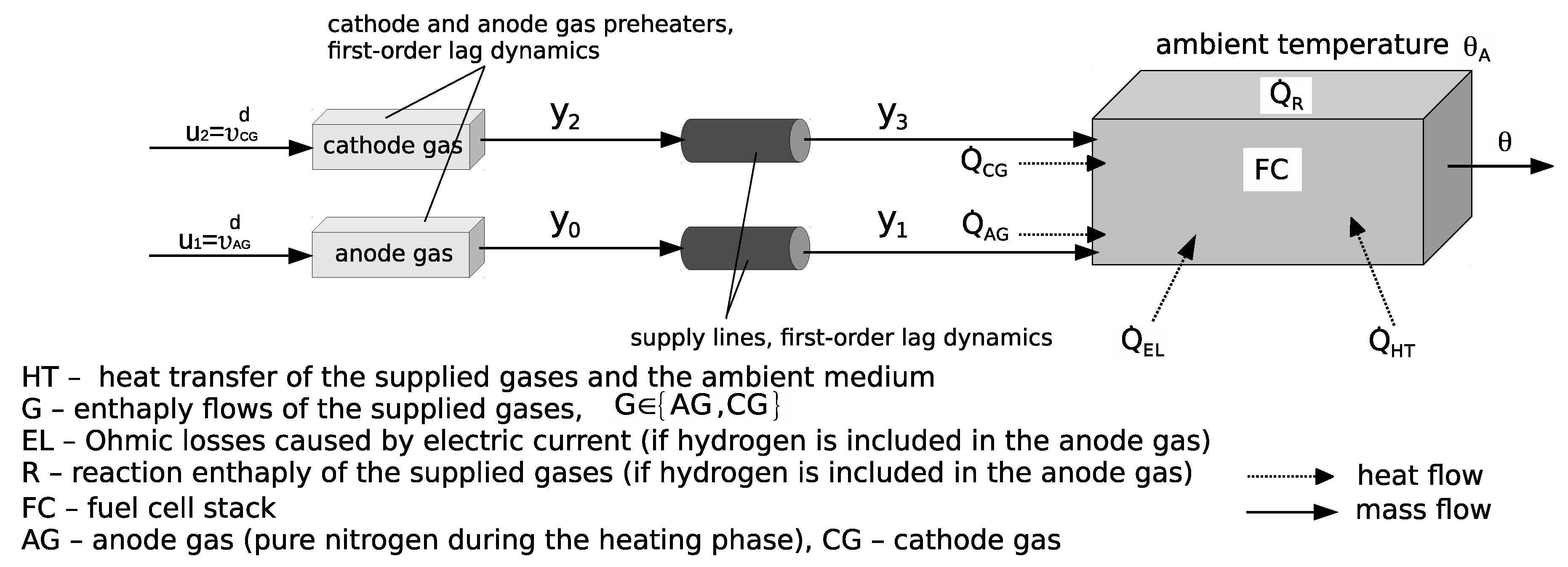
In Figure 1, a schematic overview of the SOFC test rig available at the Chair of Mechatronics at the University of Rostock is given. The key component of this test rig is an SOFC stack module with planar fuel cells in electrical series connection. The SOFC stack converts the chemical energy of the fuel gas (supplied at the anode side) into both electricity and process heat by electrochemical reactions with the oxygen contained in the cathode gas. The electrochemical energy conversion starts as soon as the required operating temperature has been reached.

For the heating phase, which begins at the ambient temperature and finishes at temperatures above $800\mathrm{K}$, two independent electric preheaters are used. During this phase, the anode gas consists of pure nitrogen (${\mathrm{N}}_2$) while air serves as the cathode gas. The time constants of both anode and cathode gas preheaters play a major role in controlling the SOFC temperature at usual operating conditions. Additionally, time constants of the corresponding supply lines (representing parasitic thermal capacities) coupling the preheater outlets with the inlet gas manifold of the SOFC stack need to be taken into account. Variations in the electric power taken from the stack module can cause local overtemperatures in the interior of the SOFC stack. These overtemperatures might lead to an accelerated degradation or even to a destruction of the SOFC stack. Hence, they need to be prevented by manipulating the cathode gas enthalpy flow with the help of a robust control strategy.

The efficiency of such controllers significantly depends on the mathematical model for the overall system. A representation of the SOFC stack by a single finite volume element with the assumption of a homogeneous temperature is sufficient for heating the system in a predefined manner. However, a spatial discretization of the temperature distribution in the interior of the stack module by a larger number volume elements is inevitable if local overtemperatures need to be detected and prevented reliably at high-temperature operating conditions. In this case, the time constants of the preheaters and of the gas supply lines need to be considered to achieve acceptable settling times for the required control procedures. As shown experimentally, linear first-order differential equations are sufficiently accurate as a mathematical model for these components.

Finite volume modelling techniques for the temperature distribution in the interior of the SOFC stack rely on an integral formulation of the energy conservation law over finitely large domains. In such a way, the partial differential equation for heat transfer can be replaced by a finite dimensional set of typically nonlinear ordinary differential equations. As pointed out above, the number of volume elements can vary. If we take one volume element for the whole stack, we obtain a single ODE for the temperature, which would be efficient wrt. the computing time, but would give us no information about temperature gradients inside the stack. Using more volume elements allows us to simulate the spatial temperature variation. If we discretise the stack by L elements in the x-axis direction, M elements in the y direction and N elements in the z direction, then the models we consider are referred to their spatial configurations $L\times M\times N$. As typical representatives, we consider a model with one volume element (configuration $1\times 1\times 1$), a model with three volume elements ($1\times 3\times 1$), and finally nine volume elements ($3\times 3\times 1$). Nonlinearities in the ODEs arise because heat capacities of the anode and cathode gases depend on temperature in a nonlinear way. The same holds for the temperature dependency of the exothermic reaction enthalpy of hydrogen.

According to the detailed description in [3], the balance equations corresponding to Figure 1 take into account the following heat flows across the boundaries of each finite volume element for the SOFC stack: heat exchange of the stack with the ambiance ${\dot{Q}}_{\mathrm{HT}}$, enthalpy flows of the supplied gases ${\dot{Q}}_{\mathrm{CG}}$, ${\dot{Q}}_{\mathrm{AG}}$, exothermic reaction enthalpies ${\dot{Q}}_{\mathrm{R}}$ (as soon as hydrogen is included in the anode gas), and Ohmic losses ${\dot{Q}}_{\mathrm{EL}}$. This leads to differential equations for the local stack temperatures with (constant) parameters that need to be identified experimentally. The control inputs of these experiments are denoted by $u_1$ and $u_2$ in Figure 1. Measured data are represented by the variables $y_i$, $i\in \{0,\dots ,3\}$, and to the stack temperature $\theta$ at specific positions in the interior of the SOFC stack. The notations like ${\nu }_{\mathrm{CG}}^{\mathrm{d}}$ stand for products of a mass flow and a temperature (e.g., for the cathode gas, “CG”). Desired values (superscript “d”) correspond to the control signals provided to our test rig.

2.2. A Short Overview of Methods with Result Verification

Methods with result verification, for example, interval arithmetic [8], affine arithmetic [18], or Taylor models [19], are constructed in such a way as to mathematically ensure a priori that the results produced by their implementation on a computer will be correct. An important effect of this view is that such methods allow us to take into account bounded uncertainty in parameters explicitly. Note that this does not include making sure that the code of the implementation is correct, which is the subject matter of code verification [20,21].

As a simple example of a method with result verification, consider obtaining a verified result of the sum $a+b$ with the help of interval analysis, where $a,b\in \mathbf{R}$ are not representable as floating point numbers. First, it is necessary to compute representations of these numbers as intervals (i.e., their enclosures) $\left[a\right]=[\underset{¯}{a},\overline{a}]$ and $\left[b\right]=[\underset{¯}{b},\overline{b}]$ with floating point bounds $\underset{¯}{a}$, $\underset{¯}{b}$, $\overline{a}$, $\overline{b}$, which is usually done by directed rounding. The lower bound is the largest representable number smaller than the exact one (rounding down, to $-\infty$, denoted by ∇). The upper bound is the smallest floating point number greater than the considered one (rounding up, to $+\infty$, ∆). The details on rigorous implementation possibilities for this procedure, even in the case when the IEEE 754 roundings to $\pm \infty$ are not available, are given in [22]. The sum is then enclosed according to the rule $\left[a\right]+\left[b\right]=\{a+b|\mathrm{for}\mathrm{all}a\in \left[a\right],b\in \left[b\right]\}=[\underset{¯}{a}+\underset{¯}{b},\overline{a}+\overline{b}]$, where the lower bound $\underset{¯}{s}=\underset{¯}{a}+\underset{¯}{b}$ has to be rounded down if it is not representable in the floating point arithmetic used on a computer, and the upper bound $\overline{s}=\overline{a}+\overline{b}$ is rounded up. In this way, the true result $s=a+b$ of the addition is always inside the interval $[\nabla \underset{¯}{s},∆\overline{s}]$ obtained using a computer, and all rounding or conversion errors are taken care of. Such rules can be devised for all basic arithmetic operations and elementary functions. They need not necessarily rely on intervals, but can take internal dependencies of variables into account, for example, in a linear way as in affine arithmetic or as a polynomial of a higher degree as in Taylor model arithmetic. To prove the correctness of results for more advanced algorithms such as those for solving algebraic or differential equations, fixed point theorems are employed. There are a number of software libraries for methods with result verification which implement the corresponding arithmetics (e.g, C-XSC [23] for intervals) and higher level algorithms (e.g., VNODE-LP [24] for solving initial value problems with the help of interval analysis).

As already mentioned in the introduction, the main disadvantage of methods with result verification is the possibility of too conservative bounds (e.g., $\pm \infty$) which appear because of the dependency problem or wrapping effect (the latter being a variation of the former). As a simple example, consider the difference of the interval $[\underset{¯}{a},\overline{a}]=\{x\in \mathbf{R}|\underset{¯}{a}\le x\le \overline{a},\underset{¯}{a}<\overline{a}\}$ and itself: $[\underset{¯}{a},\overline{a}]-[\underset{¯}{a},\overline{a}]=[\underset{¯}{a},\overline{a}]+[-\overline{a},-\underset{¯}{a}]$. According to the general definition, the true result (which is zero) is inside the interval $[\underset{¯}{a}-\overline{a},\overline{a}-\underset{¯}{a}]$ of the nonzero width $2(\overline{a}-\underset{¯}{a})$, which contains zero, but is not equal to it. In addition, the width of the resulting enclosure is twice the width of the interval $[\underset{¯}{a},\overline{a}]$ (which is equal to $\overline{a}-\underset{¯}{a}$). This happens because the general definition of the interval addition given above does not take into account that the operands are the same. Actually, we do not compute the set $\{x-x|x\in [\underset{¯}{a},\overline{a}]\}$ but rather $\{x-y|x,y\in [\underset{¯}{a},\overline{a}]\}$, which leads to the overestimation. This problem of the naive interval analysis can be solved in different ways, in particular, by “recording” dependencies (as in the Taylor model or affine approach) or by shifting the coordinate system to eliminate disturbing (unstable) factors (e.g., the QR-decomposition based method for ODEs [24]).

2.3. Verification and Validation Assessment Verification Degree

Nowadays, it is agreed [5] to consider development processes in engineering as comprising analysis, formalization, simulation, and optimisation (calibration) steps, the relations between which are characterized by the verification and validation (V&V) cycle. The cycle can be reiterated any number of times so that the task of design and formalization turns into system optimisation/calibration (including customizing) after the initial round is completed. The first stage of the cycle is to analyse the real world problem and to develop a conceptual and a formal model for it. During this phase, qualification is carried out, defined as “determination of adequacy of the conceptual model to provide an acceptable level of agreement for the domain of intended application” [5]. The second stage consists in implementing the formal model, in most cases using a computer. Here, verification is necessary, that is, making sure that the formal model is implemented correctly in the sense established by requirements devised at the previous stage. The third stage of the cycle is simulation. Validation needs to be carried out at this stage, the task of which is to compare the outcomes of the computerized model or the prototype to reality, establish the degree of similarity, and address model fidelity.

An important distinction made clear by the V&V cycle is that between the concepts of verification and validation, the exact meaning of which often depends on the considered application area. In essence, to verify a model means to prove that the model is built and simulated with the correct methods whereas the term validation denotes showing the degree of its similarity to the reality [25]. A precondition for this kind of analysis is that features of the real world problem, with respect to which the comparison is carried out, are identified at the stage of qualification. In this paper, we focus mainly on verification with the help of interval methods. However, in general, methods with result verification such as interval analysis might also offer assistance at the qualification and validation stages (cf. [26]).

At the second stage of the cycle, traditional V&V methodologies (concentrating on formal verification) suggest using benchmarks in the cases where no theoretical proof of the model and algorithm accuracy is possible and interpreting the outcome of the process of interest on these. In [6,15,16], we proposed to shift the focus on the process itself. Helped by appropriate questionnaires, users subdivide their processes into smaller tasks and classify the input/output data and algorithms, which allows us to assign a certain initial verification degree from the four-tier hierarchy shown below to the (sub-)process. Note that this hierarchy highlights our process-oriented understanding of the V&V analysis as presented in [6,15,16]. After that, the initial degree can be improved and uncertainty quantified by using a selection of specialized data types and tools. Here, interoperability with respect to data types, algorithms and used hardware is highly relevant. On the one hand, interoperable software would allow us to compute the solution in several ways in parallel and compare/interpret the outcome of these different computational models (cf. Section 4). On the other hand, a combination of different kinds of tools in one interconnected package would help to solve problems a single tool might not have the necessary means for.

A computerized system model (CSM) associated with a given real-life system has the verification degree C4 to C1 if [16]:

C4

The CSM uses standard floating point or fixed point arithmetic (the lowest verification degree).

C3

The CSM is meaningfully subdivided into its constituent parts; the numerical implementation uses at least standardized IEEE 754 floating point arithmetic; and sensitivity analysis is carried out for uncertain parameters or uncertainty is propagated through the subsystems using traditional methods (e.g., Monte-Carlo).

C2

Relevant subsystems of a CSM are implemented using tools with result verification or delivering reliable error bounds; and the convergence of numerical algorithms is proven via analytical solutions, computer-aided proofs, or fixed point theorems.

C1

The whole CSM is verified using tools and algorithms with result verification or using real number algorithms, analytical solutions, or computer-aided existence proofs; software and hardware comply with the IEEE754 and follow the interval standard P1788; uncertainty is quantified and propagated throughout the CSM using verified or stochastic (or both) approaches; and sensitivity analysis is carried out.

The degree is tagged with a minus if neither the sensitivity analysis nor uncertainty quantification were carried out. A plus alongside a degree means that the code verification (e.g, using literate programming) is performed additionally. Note that it does not necessarily mean that the result of a simulation with such a CSM would be correct. For example, a CSM categorized as having degree C3 corresponds to a situation common in small-scale engineering applications, where the model and the simulation use IEEE 754 floating point software and neither the sensitivity analysis nor uncertainty quantification are necessary.

The quality of the obtained results might also play an important role for an engineer trying to achieve a certain verification degree. Therefore, an additional quality indicator $Q_{\mathrm{id}}q$ can be used, where $q\in [0,1]$ is a real number increasing with the higher quality. The identifier id $\in \{n,u\}$ indicates whether nominal (n) or uncertain (u) parameters were considered. Different ways of computing q can be thought of. For example, the ratio $x\ge 0$ between the achieved maximum integration time and the width of the enclosure can be used in the normalized form $q:=q\left(x\right)=\frac{1}{1+e^{1-x}}$ as such a quality measure. For purely kinematic systems, the integration time is assumed to equal one (only the width is taken into account). If nominal parameters and purely floating point computations (C4, C3) without any sensitivity or uncertainty analysis are used, the quality indicator cannot be applied as defined above. In this case, an additional study is necessary to assess the reliability (e.g., using interval or stochastic approaches).

2.4. Verification Degree of ODE Based SOFC Models

Experimental identification or improvement of model parameters is an important task in the context of control-oriented SOFC modelling. As already mentioned, we are interested in control-oriented SOFC models of the general form

$$y^{\prime }=f(t,y,p),y\left(t_0\right)=y_0,$$

(1)

with the independent variable t usually assossiated with time in seconds and constant (but unknown) parameters p. To solve the identification problem, the upper bound $\overline{J}$ (if interval techniques are used) of the cost function

$$J=\sum _{k=T_b}^{T_e}\sum _{i=1}^N{\left(y_i(t_k,p)-y_{m,i}\left(t_k\right)\right)}^2$$

(2)

is minimized with respect to the parameters p. Here, $y(t_k,p)$ is the solution to the model equations (e.g., as given in Equations (5)–(9)) at the time $t_k$, $k=T_b,\cdots ,T_e$. The symbols $T_b$, $T_b$ denote the beginning and the end times in seconds, respectively. In our context, $t_k=t_{T_b},t_{T_b}+1,\cdots ,t_{T_e}$. Without loss of generality, we assume that the N states that can be measured using the SOFC test rig are the first N ones in the vector $y(t_k,p)$. The solution is obtained from the initial value problem (IVP) such as in (1) corresponding to the used SOFC model and optimised with respect to the measured values $y_{m,i}\left(t_k\right)$, $i=1\cdots N$. That is, the function J quantifies deviations between the simulated results and the measured output vector acquired with $T=T_e-T_b$ samples and a constant sampling time $h=1$ s.

According to the number of finite volume elements that are used to discretize the differential equations for the stack temperature, we might have different numbers of equations for this quantity. Until now, we considered one (MQ1), three (MQ3), and nine volume elements (MQ9) without preheaters, cf.

Table 1. Options for modelling and simulation of SOFCs.

Model	(i.a)			(i.b)			(i.c)
	(ii.a)	(ii.b)	(ii.c)	(ii.a)	(ii.b)	(ii.c)	(ii.a)	(ii.b)	(ii.c)
Models without preheaters, with quadratic $c\left(\theta \right)$, 1, 3 and 9 volume elements, resp.
MQ1	not possible			[27]	[28]		[26,29]
MQ3	not possible			[27]	[7]		[29]	too slow	too slow
MQ9	not possible			[27]	future work		too slow
Model without preheaters, with linear $c\left(\theta \right)$, 1 volume element
ML1	[26]			not interesting			not interesting
Models with preheaters, quadratic $c\left(\theta \right)$, 1 and 3 volume elements, resp.
MPQ1	not possible			[4]	future work		future work
MPQ3	not possible			[4]	future work		future work
Model with piecewise constant preheaters, linear $c\left(\theta \right)$, 1 volume element
MPL1	this paper			this paper			not interesting
Models with preheaters, constant $c\left(\theta \right)$, 1, 3 and 9 volume elements, resp.
MPC1	this paper						not interesting
MPC3	future work						not interesting
MPC9	too complex			future work			too slow

and [27]. Finer discretisations are possible in principle but are expensive computationally. Notations such as MQ1 are labels for the corresponding models (e.g., the one with a single volume element) and allow us to refer to them in a compact form according to the following system. The letter M just means model. Q,L,C mean using the approximations to the heat capacities by a quadratic, a linear and a constant polynomial. Letter P indicates the use of the model for the preheaters, and the number denotes the number of volume elements. An empirically motivated additional condition is induced by the accuracy of the measurements:

$$y_i\left(t_k\right)\subseteq [y_{m,i}\left(t_k\right)-c_i,y_{m,i}\left(t_k\right)+c_i]=:[\Delta y_m\left(t_k\right)]\text{for}k=T_b,\cdots ,T_e,i=1\cdots N$$

(3)

with constants $c_i>0$ chosen in accordance with the sensor data sheets of the actual SOFC test rig.

The models described above might have the following basic forms depending on:

(i)

the way the simulated solution $y(t_k,p)$ of the IVP is obtained in Equation (2):

(i.a)

$y(t_k,p)$ is computed analytically,

(i.b)

$y(t_k,p)$ is approximated by an analytic expression (e.g., using the Euler method) and the approximation error is neglected, which is justified in cases in which the integration step size is smaller by several orders of magnitude than the smallest time constant of an asymptotically stable ODE system (cf. Equation (4)), and

(i.c)

$y(t_k,p)$ is computed using a “black box” numerical solver (no explicit expression for the solution); and

(ii)

the kind of used arithmetic:

(ii.a)

traditional floating point arithmetic,

(ii.b)

interval arithmetic, and

(ii.c)

affine arithmetic, Taylor models, etc.

Generally, forms (i.a) and (i.c) combined with (ii.b) or (ii.c) correspond to the complete verification of the model (C1), if optimisation is carried out in a completely verified way. If a certain best suitable interval vector is chosen from the list of candidates produced by global optimisation according to a heuristic technique, then the corresponding degree is C2.

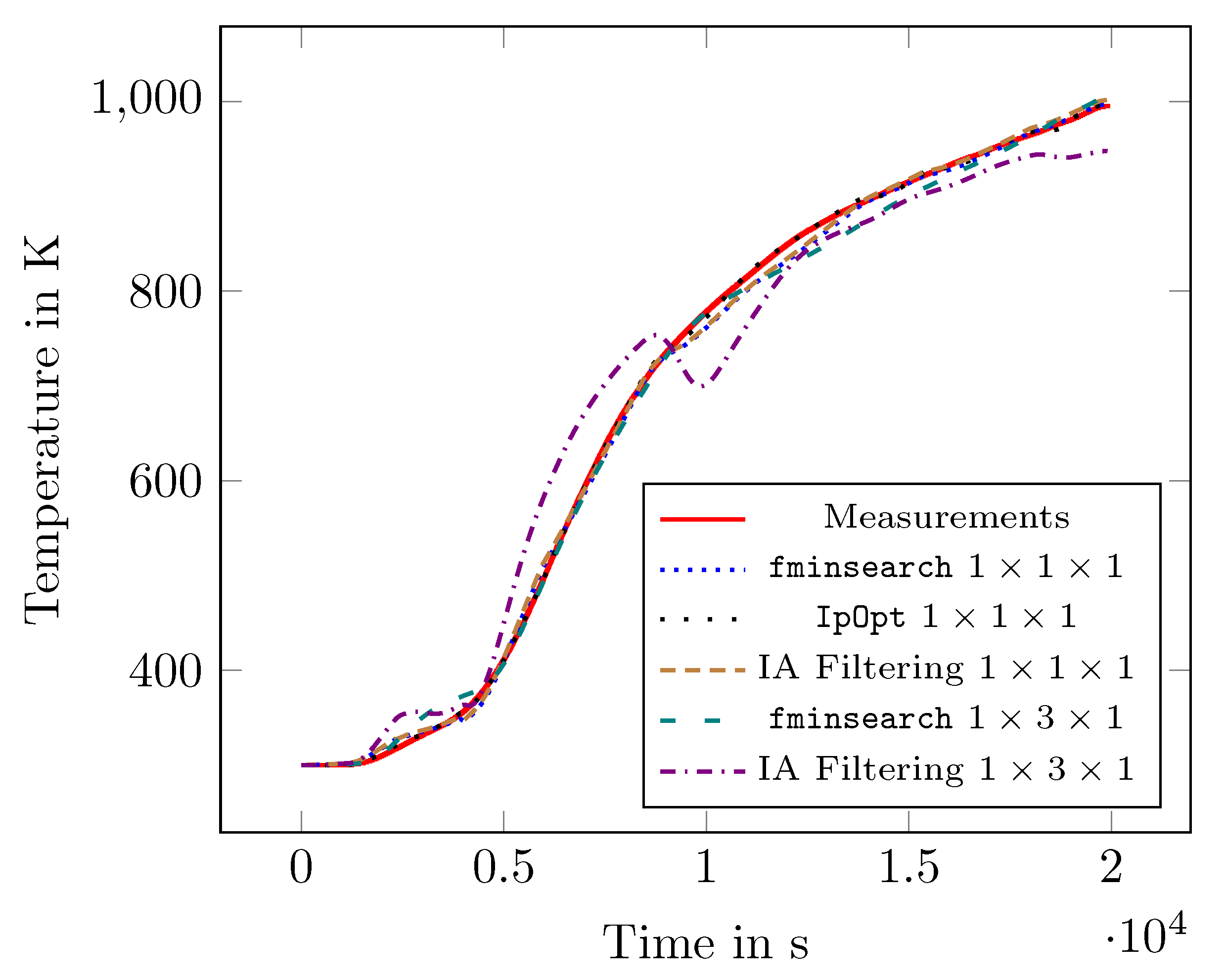
In most of our recent publications (e.g., [7,28]), we solved the global optimisation problem in Equation (2) by verified approximation ((i.b) with (ii.b)): The true solution $y\left(t\right)$ of the IVP was approximated by the explicit Euler method in its interval version taking into account numerical errors but not the discretisation error as $\left[y^{\left(k\right)}\right]:=\left[y^{(k-1)}\right]+h·f(\left[y^{(k-1)}\right],\left[p\right])$, where f denotes the right-hand side of the IVP (componentwise). The interval approximation $\left[y^{\left(k\right)}\right]$ at $t_k$ was substituted for the exact solution $y\left(t_k\right)$ in the cost function in Equation (2) and the discretisation error ignored. In our setup, the sampling time $h=1$ s is by at least two orders of magnitude smaller than the dominant time constant of the thermal process, that is, $\left[y^{\left(k\right)}\right]$ was an acceptable approximation of the true solution $y\left(t_k\right)$. Although we could not verify the whole process by applying interval optimisation procedures in this case, the approximated cost function

$$J_{app}=\sum _{k=T_b+1}^{T_e}\sum _{i=1}^N{\left(y_i^{(k-1)}-y_{m,i}\left(t_k\right)+h·f(y_i^{(k-1)},p)\right)}^2,$$

(4)

where $y^{\left(T_b\right)}$ is the initial condition, was evaluated in a verified way and optimised using an interval algorithm, resulting in the verification degree of C2 for MQ1 and MQ3. Note that the first (and second) derivatives of $J_{app}$ were computed exactly with the help of algorithmic differentiation. In Figure 2, the results of this study are shown.

As explained above, fully verified versions of the models for the parameter identification can appear if Variant (i.c) with (ii.b) is used. That means that the true solution $y(t,p)$ needs to be enclosed numerically by a verified IVP solver. For the Variant (i.c), it is more difficult to compute the derivatives $\partial J/\partial p$ of the cost function J in general, because it requires solving an additional IVP to obtain the sensitivities of the solution. This possibility was explored in [26,29]. The general outcome here is that although the quality of the obtained parameters improves in this case, the computing times become too high even for MQ1. On the one hand, there is no possibility to use parallelisation on the GPU (and even on a multicore CPU) due to the lack of corresponding implementations (e.g., for verified IVP solvers). On the other hand, the IVP becomes more complex since the derivatives cannot be calculated by using algorithmic differentiation. The overall verification degree is still C2 in this case since high computing times prevented the summation over the whole interval $[T_b,T_e]$ and necessitated partial optimisation over smaller time intervals.

ODEs for the SOFC models MQ1, MQ3, MQ9 cannot be solved analytically in general. This is mainly due to the temperature dependent heat capacities of the gases. For example, the heat capacity $c_{\mathrm{N}2}\left(\theta \right)$ of nitrogen is usually approximated by a second-degree polynomial as $c_{\mathrm{N}2}^{\mathrm{app}}\left(\theta \right)=c_{\mathrm{N}2,0}+c_{\mathrm{N}2,1}\theta +c_{\mathrm{N}2,2}{\theta }^2$, where $c_{\mathrm{N}2,0}$, $c_{\mathrm{N}2,1}$, $c_{\mathrm{N}2,2}$ are constants (time-invariant parameters to be identified later). This leads to the right-hand side of the ODE which is cubic in temperature. In [26], we showed how to compute an analytical solution for the model with one volume element for the temperature (and without preheaters) if all heat capacities and the reaction enthalpy are considered to be linear (that is, the parameters $p_i=c_{·,2}$ with the last index 2 are neglected), the model which we call ML1. With more volume elements for the temperature, we cannot solve the resulting higher dimensional ODEs analytically even if the dependency of the heat capacities on the temperature is linearized, since the right-hand sides of the IVPs have (mixed) quadratic dependencies on the individual temperature states. In Table 1, an overview of possibilities along with the options we covered is given.

The model can be simplified even further if we assume that the heat capacities of the involved gases are constant. This results in an overall set of ODEs which are linear in temperature with constant coefficients, so that an analytical solution can be obtained in all cases of the finite volume discretisation, at least in theory. Additionally, we take into account two preheaters, each described by two linear ODEs, each of the first order. As a first study of usefulness of such models, we consider only one volume element for the temperature of the stack (MPQ1, MPL1 and MPC1).

Note that although the control-oriented SOFC models are less complex than those based on partial differential equations, they are still complex enough so that their treatment with general-purpose verified global optimisation software is next to impossible. For example, the summation in Equation (2) is carried out for T = 17,628 measurements (corresponding to the heating stage of the experiment), which causes numerical problems even in the usual floating point based case.

3. Simplifying the Models

The previous section demonstrated that a trade-off between a high verification degree and an acceptable computing time is necessary. That is, if we would like to arrive at high verification degrees in a real-time simulation or control, we might need to simplify the models, the possibilities for which are described in this section. Besides, we study the quality of such models and try to find their areas of validity in an empirical way in the next section.

In this paper, we consider the nitrogen as the only anode gas for the heating phase without any chemical reactions of gases. Besides, we work with a single volume element to describe the temperature of the stack as a whole. In [26], we pointed out ways to simplify the model for the SOFC stack with one volume element and no preheaters. In this paper, we consider two preheaters, since this improves the overall quality of SOFC models from the point of view of their control. Parameters denoted by $\dot{m}$ describe mass flows of, for example, nitrogen and are assumed to be piecewise constant (applies to all control variables from

Table 2. Model parameters, control inputs and state variables.

Parameters (to Identify)
${\alpha }_i$, ${\alpha }_j$, ${\alpha }_k$	coefficients of heat convection in $\frac{\mathrm{W}}{{\mathrm{m}}^2·\mathrm{K}}$
$c_{\mathrm{N}2,0}$, $c_{\mathrm{N}2,1}$	heat capacity of nitrogen as $c_{\mathrm{N}2}\left(\theta \right)=c_{\mathrm{N}2,0}+c_{\mathrm{N}2,1}·\theta$ in $\frac{\mathrm{J}}{\mathrm{kg}·\mathrm{K}}$
$c_{\mathrm{CG},0}$, $c_{\mathrm{CG},1}$	heat capacity of the cathode gas as $c_{\mathrm{CG}}\left(\theta \right)=c_{\mathrm{CG},0}+c_{\mathrm{CG},1}·\theta$ in $\frac{\mathrm{J}}{\mathrm{kg}·\mathrm{K}}$
$T_{\mathrm{AG}}^{\mathrm{inv}}$	inverse time constant of the anode gas preheater in s${}^{-1}$
$T_{\mathrm{CG}}^{\mathrm{inv}}$	inverse time constant of the cathode gas preheater in s${}^{-1}$
$T_{\mathrm{SL},\mathrm{AG}}^{\mathrm{inv}}$	inverse time constant of the anode gas supply line in s${}^{-1}$
$T_{\mathrm{SL},\mathrm{CG}}^{\mathrm{inv}}$	inverse time constant of the cathode gas supply line in s${}^{-1}$
c	specific heat capacity of the stack module in $\frac{\mathrm{J}}{\mathrm{kg}·\mathrm{K}}$
m	mass of the stack module in kg
$c_m^{\mathrm{inv}}$	$=1/(c·m)$
Variables
$y_0=v_{\mathrm{N}2}$	product of the mass flow and the temperature ${\dot{m}}_{\mathrm{N}2}^{\mathrm{in}}·{\theta }_{\mathrm{N}2}$ of the anode gas (nitrogen) at the preheater outlet in $\frac{\mathrm{kg}·\mathrm{K}}{\mathrm{s}}$
$y_1=v_{\mathrm{N}2}^{\mathrm{in}}$	product ${\dot{m}}_{\mathrm{N}2}^{\mathrm{in}}·{\theta }_{\mathrm{N}2}^{\mathrm{in}}$ for the nitrogen at the stack inlet in $\frac{\mathrm{kg}·\mathrm{K}}{\mathrm{s}}$
$y_2=v_{\mathrm{CG}}$	product ${\dot{m}}_{\mathrm{CG}}^{\mathrm{in}}·{\theta }_{\mathrm{CG}}$ for the cathode gas at the preheater outlet in $\frac{\mathrm{kg}·\mathrm{K}}{\mathrm{s}}$
$y_3=v_{\mathrm{CG}}^{\mathrm{in}}$	product ${\dot{m}}_{\mathrm{CG}}^{\mathrm{in}}·{\theta }_{\mathrm{CG}}^{\mathrm{in}}$ for the cathode gas at the stack inlet in $\frac{\mathrm{kg}·\mathrm{K}}{\mathrm{s}}$
$\theta$	temperature of the stack in K
Control Inputs
${\dot{m}}_{\mathrm{N}2}^{\mathrm{in}}$	mass flow of anode gas in $\frac{\mathrm{kg}}{\mathrm{s}}$ (recorded data)
${\dot{m}}_{\mathrm{CG}}^{\mathrm{in}}$	mass flow of cathode gas in $\frac{\mathrm{kg}}{\mathrm{s}}$ (recorded data)
${\theta }_A$	ambient temperature in K
${\theta }_{\mathrm{AG}}^{\mathrm{d}}$	desired temperature of the anode gas in K (recorded data)
${\theta }_{\mathrm{CG}}^{\mathrm{d}}$	desired temperature of the cathode gas in K(recorded data)
$u_1=v_{\mathrm{N}2}^{\mathrm{d}}$	desired $v_{\mathrm{N}2}={\theta }_{\mathrm{AG}}^{\mathrm{d}}·{\dot{m}}_{\mathrm{N}2}^{\mathrm{in}}$ in $\frac{\mathrm{kg}·\mathrm{K}}{\mathrm{s}}$
$u_2=v_{\mathrm{CG}}^{\mathrm{d}}$	desired $v_{\mathrm{CG}}={\theta }_{\mathrm{CG}}^{\mathrm{d}}·{\dot{m}}_{\mathrm{CG}}^{\mathrm{in}}$ in $\frac{\mathrm{kg}·\mathrm{K}}{\mathrm{s}}$

). They are spatially invariant in the complete test rig; there are no relevant storage effects due to compressibility. Note that although the notation $\dot{x}$ denotes the derivative of x wrt. time and $\dot{m}$ could have been modeled using appropriate IVPs, we use the information from measurements to describe these values if they are shown in Table 2. All other parameters are constant. Here, we consider the models MPC1 and MPL1 in detail, cf. Table 1.

The simplified model MPL1 relies on linear polynomial approximations for the heat capacities. However, this results in a Riccati differential equation if we assume that preheater states are not constant inside the considered time interval (of the width 1s in our case). This differential equation can be transformed into a system of two linear differential equations with non-constant coefficients which is not easy to solve analytically in our case. For piecewise constant preheater states, it is possible to calculate the analytical solution similarly to [26]. In this paper, we study the properties of MPL1 in addition to MPC1.

3.1. Simplified Model MPC1: Constant Heat Capacities

The system of ODEs we can derive if we assume all heat capacities to be constant in temperature (MPC1) is shown below:

$$\begin{array}{ccc}\hfill {\dot{y}}_0& =& T_{\mathrm{AG}}^{\mathrm{inv}}·(u_1-y_0)\hfill \end{array}$$

(5)

$$\begin{array}{ccc}\hfill {\dot{y}}_1& =& T_{\mathrm{SL},\mathrm{AG}}^{\mathrm{inv}}·(y_0-y_1)\hfill \end{array}$$

(6)

$$\begin{array}{ccc}\hfill {\dot{y}}_2& =& T_{\mathrm{CG}}^{\mathrm{inv}}·(u_2-y_2)\hfill \end{array}$$

(7)

$$\begin{array}{ccc}\hfill {\dot{y}}_3& =& T_{\mathrm{SL},\mathrm{CG}}^{\mathrm{inv}}·(y_2-y_3)\hfill \end{array}$$

(8)

$$\begin{array}{ccc}\hfill \dot{\theta }& =& -c_m^{\mathrm{inv}}·(k_{\mathrm{const}}-(c_{\mathrm{CG},0}·y_3+c_{\mathrm{N}2,0}·y_1)+k_{\mathrm{lin}}\theta ),\hfill \end{array}$$

(9)

with

$$\begin{array}{cc}\hfill k_a& =234000{\alpha }_i+448500{\alpha }_j+345000{\alpha }_k,\hfill \\ \hfill k_{\mathrm{const}}& =-{\theta }_A{k}_a,\hfill \\ \hfill k_{\mathrm{lin}}& =k_a+{\dot{m}}_{\mathrm{CG}}^{\mathrm{in}}·c_{\mathrm{CG},0}+{\dot{m}}_{\mathrm{N}2}^{\mathrm{in}}·c_{\mathrm{N}2,0},\hfill \end{array}$$

and initial conditions $y_i\left(t_0\right)=y_i^{\mathrm{ic}}$, $i=0,1,2,3$, $\theta \left(t_0\right)={\theta }^{\mathrm{ic}}$. That is, we obtain a linear set of ODEs for the temperature including the preheater states from the energy balance equations that were explained in Section 2.1. Physical units of the numerical values included in the defitnion of $k_a$ are not listed explicitly, because all parameters are assumed to be given in SI derived units. Equations (5)–(6) describe the first preheater (for the anode gas), Equations (7)–(8) the second (for the cathode gas), and Equation (9) the stack temperature.The meaning of all parameters, variables, and control inputs is given in Table 2. For $T_{\mathrm{SL},\mathrm{AG}}^{\mathrm{inv}}\ne T_{\mathrm{AG}}^{\mathrm{inv}}$, there is a simple analytical solution to the model according to

$$\begin{array}{ccc}\hfill y_0\left(t\right)& =& u_1-(u_1-y_0^{\mathrm{ic}})e^{-T_{\mathrm{AG}}^{\mathrm{inv}}(t-t_0)}\hfill \end{array}$$

(10)

$$\begin{array}{ccc}\hfill y_1\left(t\right)& =& u_1-\frac{T_{\mathrm{SL},\mathrm{AG}}^{\mathrm{inv}}}{T_{\mathrm{SL},\mathrm{AG}}^{\mathrm{inv}}-T_{\mathrm{AG}}^{\mathrm{inv}}}(u_1-y_0^{\mathrm{ic}})e^{-T_{\mathrm{AG}}^{\mathrm{inv}}(t-t_0)}+k_{\mathrm{N}2}{e}^{-T_{\mathrm{SL},\mathrm{AG}}^{\mathrm{inv}}(t-t_0)}\hfill \end{array}$$

(11)

for the anode gas preheater, where $k_{\mathrm{N}2}=y_1^{\mathrm{ic}}-u_1+\frac{T_{\mathrm{SL},\mathrm{AG}}^{\mathrm{inv}}}{T_{\mathrm{SL},\mathrm{AG}}^{\mathrm{inv}}-T_{\mathrm{AG}}^{\mathrm{inv}}}(u_1-y_0^{\mathrm{ic}})$. If $T_{\mathrm{SL},\mathrm{AG}}^{\mathrm{inv}}=T_{\mathrm{AG}}^{\mathrm{inv}}$, we obtain a different formula for $y_1\left(t\right)$:

$$y_1\left(t\right)=u_1-\left(u_1-y_1^{\mathrm{ic}}-T_{\mathrm{AG}}^{\mathrm{inv}}(u_1-y_0^{\mathrm{ic}})(t-t_0)\right)e^{-T_{\mathrm{AG}}^{\mathrm{inv}}(t-t_0)}.$$

(12)

The solution for the cathode gas preheater looks the same, only the parameters are different: all labels “N2” (or AG) should be changed to “CG”.

The solution for the temperature can be obtained easily after inserting the corresponding expressions for $y_3\left(t\right)$ and $y_1\left(t\right)$ into Equation (9) by variable separation and variation of the constant. It has the general form

$$\theta \left(t\right)={\mathcal{I}}_{\mathrm{N}2}\left(t\right)+{\mathcal{I}}_{\mathrm{CG}}\left(t\right)+k_{\theta }{e}^{-c_m^{\mathrm{inv}}·k_{\mathrm{lin}}(t-t_0)}-\frac{k_{\mathrm{const}}}{k_{\mathrm{lin}}},$$

(13)

where

$$\begin{array}{cc}\hfill {\mathcal{I}}_{\mathrm{N}2}\left(t\right)& :=\frac{u_1·c_{\mathrm{N}2,0}}{k_{\mathrm{lin}}}+c_m^{\mathrm{inv}}·c_{\mathrm{N}2,0}(-\frac{T_{\mathrm{SL},\mathrm{AG}}^{\mathrm{inv}}}{(T_{\mathrm{SL},\mathrm{AG}}^{\mathrm{inv}}-T_{\mathrm{AG}}^{\mathrm{inv}})(c_m^{\mathrm{inv}}{k}_{\mathrm{lin}}-T_{\mathrm{AG}}^{\mathrm{inv}})}(u_1-y_0^{\mathrm{ic}})e^{-T_{\mathrm{AG}}^{\mathrm{inv}}(t-t_0)}\hfill \\ & +\frac{k_{\mathrm{N}2}}{c_m^{\mathrm{inv}}{k}_{\mathrm{lin}}-T_{\mathrm{SL},\mathrm{AG}}^{\mathrm{inv}}}{e}^{-T_{\mathrm{SL},\mathrm{AG}}^{\mathrm{inv}}(t-t_0)}),\hfill \end{array}$$

${\mathcal{I}}_{\mathrm{CG}}\left(t\right)$ analogously, and $k_{\theta }={\theta }^{\mathrm{ic}}-{\mathcal{I}}_{\mathrm{CG}}\left(t_0\right)-{\mathcal{I}}_{\mathrm{N}2}\left(t_0\right)+\frac{k_{\mathrm{const}}}{k_{\mathrm{lin}}}$. Note that only the situation in which $T_{\mathrm{SL},\mathrm{AG}}^{\mathrm{inv}}\ne T_{\mathrm{AG}}^{\mathrm{inv}}$ and $T_{\mathrm{SL},\mathrm{CG}}^{\mathrm{inv}}\ne T_{\mathrm{CG}}^{\mathrm{inv}}$ is relevant for the considered SOFC test rig. (Note that an analytical formula for $\theta \left(t\right)$ can be obtained also for the case of identical time constants using the same technique as above.) If we assume that the preheater outlet temperatures are piecewise constant in time and employ the recorded sensor data instead of the dynamic model given by Equations (5)–(8), the corresponding solution for the temperature becomes much simpler:

$$\theta \left(t\right)=-\frac{{\tilde{k}}_{\mathrm{const}}}{k_{\mathrm{lin}}}+\left({\theta }^{\mathrm{ic}}+\frac{{\tilde{k}}_{\mathrm{const}}}{k_{\mathrm{lin}}}\right)·e^{-c_m^{\mathrm{inv}}·k_{\mathrm{lin}}·(t-t_0)},$$

(14)

where ${\tilde{k}}_{\mathrm{const}}=-{\theta }_A·k_a-(c_{\mathrm{CG},0}·y_3^{\mathrm{ic}}+c_{\mathrm{N}2,0}·y_1^{\mathrm{ic}})$.

Because the control variables are piecewise constant, the IVP is solved separately in each time interval $[t_{n-1},t_n]$, $n=T_b+1,\cdots ,T_e$. The initial values in the next step are the results from the previous step, $t_0=t_n$. If the possibility (ii.b) is used, we work with the interval hull of the values of these control variables, because we do not know the exact value inside $[t_{n-1},t_n]$, only in $t_{n-1}$ and $t_n$.

The same approach is possible if larger numbers of volume elements are used for modelling the temperature of the SOFC stack. However, the results in Section 4 suggest that the expressions for the exact solutions are so complex that there is almost no gain in using them from the point of view of the computing time. That is, option (i.a) might work too slow for MPC9, for example.

Note that using the numerical computing environment MATLAB did not work very well for obtaining closed-form expressions (which had to be derived “by hand”). Although it was possible to compute the closed-form solution using MATLAB for $y_0$, $y_1$, $y_2$ and $y_3$, the expressions were numerically unstable, leading to overflows with increasing times t. The expression for the temperature $\theta$ could not be computed in MATLAB for dynamic preheater representations. A MATLAB solution under the assumption that the preheater states are piecewise constant (the case similar to Equation (14)) was also numerically unstable.

3.2. Simplified Model MPL1: Linear Heat Capacities

Although we now take into account two preheaters in the overall model, this does not change the general approach to obtain the exact solution in case of linearly approximated heat capacities. Equations (5)–(8) stay the same. The equation for the temperature turns into

$$\dot{\theta }=-c_m^{\mathrm{inv}}·(k_{\mathrm{const}}\left(t\right)+k_{\mathrm{lin}}\left(t\right)\theta +k_{\mathrm{sq}}\left(t\right){\theta }^2),$$

(15)

where $k_{\mathrm{const}}\left(t\right)$, $k_{\mathrm{lin}}\left(t\right)$ depend on time and ${\theta }^2$ appears on the right-hand side of the equation with the constant coefficient $k_{\mathrm{sq}}\left(t\right)$:

$$\begin{array}{cc}\hfill k_{\mathrm{const}}\left(t\right)& =-{\theta }_A{k}_a-(y_3\left(t\right)c_{\mathrm{CG},0}+y_1\left(t\right)c_{\mathrm{N}2,0})\left(k_a\mathrm{as}\mathrm{in}\mathrm{Section}3.1\right),\hfill \\ \hfill k_{\mathrm{lin}}\left(t\right)& =k_{+}{\dot{m}}_{\mathrm{CG}}^{\mathrm{in}}·c_{\mathrm{CG},0}+{\dot{m}}_{\mathrm{N}2}^{\mathrm{in}}·c_{\mathrm{N}2,0}-(y_3\left(t\right)c_{\mathrm{CG},1}+y_1\left(t\right)c_{\mathrm{N}2,1}),\hfill \\ \hfill k_{\mathrm{sq}}\left(t\right)& ={\dot{m}}_{\mathrm{CG}}^{\mathrm{in}}·c_{\mathrm{CG},1}+{\dot{m}}_{\mathrm{N}2}^{\mathrm{in}}·c_{\mathrm{N}2,1}.\hfill \end{array}$$

Note that we have two additional parameters $c_{\mathrm{CG},1}$, $c_{\mathrm{N}2,1}$ now, resulting from the fact that we represent heat capacities of gases as linear polynomials in temperature: $c_{\mathrm{N}2}\left(\theta \right)=c_{\mathrm{N}2,0}+c_{\mathrm{N}2,1}·\theta$, $c_{\mathrm{CG}}\left(\theta \right)=c_{\mathrm{CG},0}+c_{\mathrm{CG},1}·\theta$. Equation (15) is a Riccati equation. Since $k_{\mathrm{sq}}$ does not depend on time in our case because gas mass flows are constant, it can be transformed into a system of the following linear ODEs with non-constant coefficients:

$${\left(\begin{array}{c}{y}_4\\ y_5\end{array}\right)}^{\prime }=\left(\begin{array}{cc}0& 1\\ -{\left(c_m^{\mathrm{inv}}\right)}^2{k}_{\mathrm{const}}\left(t\right)k_{\mathrm{sq}}& -c_m^{\mathrm{inv}}{k}_{\mathrm{lin}}\left(t\right)\end{array}\right)·\left(\begin{array}{c}{y}_4\\ y_5\end{array}\right),$$

(16)

where the temperature $\theta$ equals ${\displaystyle \frac{y_5}{c_m^{\mathrm{inv}}{k}_{\mathrm{sq}}{y}_4}}$. It is probably impossible to find closed-form solutions to that set of equations in our case because the matrix in Equation (16) does not even necessarily commute with itself for given points of time t. Therefore, we assumed that the preheaters behaved as piecewise constant functions similarly to externally specified control variables. Due to new sensor material (in comparison to [26]), it was possible to measure the values of $y_1$ and $y_3$ in all relevant points of time. The closed-form solution for the temperature equation with–now constant–coefficients $k_{\mathrm{const}}$, $k_{\mathrm{lin}}$ with $y_1\left(t\right)=y_1^{\mathrm{meas}}$, $y_3\left(t\right)=y_3^{\mathrm{meas}}$ is given in dependence on $D=k_{\mathrm{lin}}^2-4k_{\mathrm{const}}{k}_{\mathrm{sq}}$ according to

$$D>0:{\displaystyle \theta \left(t\right)=\frac{1}{k_{\mathrm{sq}}}\left(\frac{\sqrt{D}}{1-e^{-c_m^{\mathrm{inv}}(t-t_0)\sqrt{D}}·\left({\displaystyle 1-\frac{2\sqrt{D}}{2k_{\mathrm{sq}}{\theta }^{\mathrm{ic}}+k_{\mathrm{lin}}+\sqrt{D}}}\right)}-\frac{k_{\mathrm{lin}}+\sqrt{D}}{2}\right)}$$

$$D<0:{\displaystyle \theta \left(t\right)=\frac{\sqrt{-D}tan(-\frac{\sqrt{-D}}{2}{c}_m^{\mathrm{inv}}(t-t_0)+{\theta }^c)-k_{\mathrm{lin}}}{2k_{sq}}},{\displaystyle {\theta }^c=\mathrm{atan}\left(\frac{2k_{\mathrm{sq}}{\theta }^{\mathrm{ic}}+k_{\mathrm{lin}}}{\sqrt{-D}}\right)}$$

$$D=0:{\displaystyle \theta \left(t\right)=\frac{2{\theta }^{\mathrm{ic}}+k_{\mathrm{lin}}/k_{\mathrm{sq}}}{2+c_m^{\mathrm{inv}}(t-t_0)(2k_{\mathrm{sq}}{\theta }^{\mathrm{ic}}+k_{\mathrm{lin}})}-\frac{k_{\mathrm{lin}}}{2k_{\mathrm{sq}}}}\left(\mathrm{improbable}\mathrm{in}\mathrm{our}\mathrm{case}\right)$$

From the definitions for $k_{\mathrm{const}}$, $k_{\mathrm{lin}}$, $k_{\mathrm{sq}}$ and the data, it is likely (but not certain) that D is positive. Nonetheless, it is necessary to check the sign in the corresponding parameter identification/simulation routines and choose the solution branch accordingly. The results of parameter identification using this multi-branch analytical expression to obtain new parameter sets are given in [31]. In this paper, we use these expressions only with parameter values computed in MATLAB.

Note that including dynamic representations for the preheaters instead of replacing their behaviour by measured values is preferable for the design of controllers which take into account the thermal system model as a whole. After the introduction of suitable sample and hold elements, the Equations (5)–(8) could still be used in a piecewise constant way; however, the difference to the “true” solution of the Riccati equation would be considerable. To identify the parameters for the preheaters and the stack together and to study the usefulness of such a variant is a topic for the future research.

4. Numerical Results

In [7,28], we introduced an environment VERICELL for reliable simulation and testing of SOFC models using different kinds of arithmetics, including interval, affine, and Taylor model ones. This environment is based on the framework UniVerMeC [32] which decouples higher-level processes from the underlying arithmetics. In particular, this feature allows us to work with the identical description of a model using different kinds of arithmetics (interoperability mentioned in Section 2.3). UniVerMeC, which is freely available (e.g., via an email to St. Kiel), is implemented using a relaxed layered structure (a layer can be skipped). The bottom layer core provides access to floating point, interval, and affine arithmetic as well as to Taylor models, which share a common interface. The next layer, function, allows us to represent scalar and vector-valued functions uniformly if their mathematical sense is supplied according to the formalization from [32]. This concept helps to evaluate a function with all arithmetics supported at the core layer. We introduce abstractions for derivatives, slopes, Taylor coefficients or contractors at this level, a list which advanced users can extend if necessary. The third layer is responsible for defining models in the framework, for example, the IVPs from Table 1. It merges the relevant abstractions provided at the previous two layers into one entity. Specialized data structures for higher-level algorithms are at the fourth level, for example, those for special types of search space decomposition used in optimisation. Actual algorithms are implemented at the topmost level. UniVerMeC offers its own global optimisation algorithm GlobOpt based on that described in [33] which can be employed for parameter identification of SOFC models. Additionally, external software such as IVP solvers or further optimisers can be interfaced at this level. In particular, we incorporate the IVP solver vode [34] to cover form (ii.a) from Subsection 2.4 as well as VNODE-LP [24] and ValEncIA-IVP [35] to cover (ii.b). For non-verified floating point optimisation, we interface the interior-point tool IPOPT [30].

Owing to this internal structure, different algorithms, for example, floating point or interval IVP solvers, can operate with the same model representation, which reduces the amount of work for users and their potential transformation errors as well as ensures a higher degree of interchangeability and comparability for the employed software. Besides, verified and non-verified methods can be meaningfully mixed with its help. For example, the values of parameters obtained by optimizing a model using a floating point tool IPOPT can be validated by running a verified solver for the IVP using them and checking with interval arithmetic whether the obtained enclosures fulfill the condition in Equation (3). Moreover, simulations for models from Table 1 in forms (i.a) (with (ii.a) or (ii.b)) and (i.b) (with (ii.a) or (ii.b)) can be made faster by using the GPU [7]. Finally, different software libraries (e.g., for intervals or Taylor models) can be used without the need to rewrite the whole program.

The aim of numerical experiments here is to study the simplified models from Section 3 with respect to their accuracy and performance. Our particular goals are, first, to decide whether MPC1 and MPL1 describe the measurements well enough (if not, the similarity areas are of interest). Second, we are interested in any differences in the quality of the obtained parameters between variants with and without the exact solution ((i.a) versus (i.b)) for MPC1/MPL1.

We have two settings in our numerical experiments, which we call S-MATLAB and S-VERICELL in the following. S-MATLAB corresponds to simulation/optimisation in MATLAB and SIMULINK. The parameters of the system are optimised by the routine fminsearch [36] which is based on the derivative-free Nelder–Mead simplex method. Instead of a single run using Equation (2) with Equations (5)–(9), two separate runs were performed to optimise parameters of the anode and cathode gas preheaters first (only for Equation (6) and Equation (8)) and, after that, for the temperature of the stack (Equation (9)). In the latter case, we did not use the dynamic information about the preheaters from Equations (5)–(8) but rather the corresponding measurements. The reason for these two separate runs is that the magnitudes of the variables $y_1$, $y_3$ and $\theta$ are too different (of orders ${10}^{-2}$, ${10}^{-1}$, and ${10}^3$, respectively). In this setting, the degree of verification is C3− (corresponding to (i.b) + (ii.a)). In the S-VERICELL setting, we performed the optimisation for MPC1 in one run, taking into account only the model equations without additional measurements according to

$$\sum _{t_k=T_b}^{T_e}\left({\displaystyle {\left(\frac{y_1\left(t_k\right)-y_{m,1}\left(t_k\right)}{{\sigma }_1}\right)}^2+{\left(\frac{y_3\left(t_k\right)-y_{m,3}\left(t_k\right)}{{\sigma }_3}\right)}^2+{\left(\frac{\theta \left(t_k\right)-y_{m,4}\left(t_k\right)}{{\sigma }_4}\right)}^2}\right)$$

(17)

(a weighted sum, ${\sigma }_i$, $i=1,3,4$, is the mean value of the corresponding measurement data $y_{m,i}$ over $[T_b,T_e]$) as a comparison. Since we could not take into account the models for the preheaters in case of MPL1 (see Section 3.2), we identified only the parameters for the SOFC stack temperature here. For both MPC1 and MPL1, we employed the floating point based tool IPOPT for parameter identification and an interval IVP solver VNODE-LP for simulation, resulting in the overall verification degree of C2− (situation where (ii.a) is combined with (ii.b)). Besides, we do not only consider (i.b), the solution obtained by the Euler method, but also (i.a), the exact solution.

In both settings, $T_b=362$ and $T_e=18000$, which corresponds to the heating stage from the data recorded during an experiment on the SOFC test rig. We identify eight parameters for MPC1: ${\alpha }_i$ (${\alpha }_i={\alpha }_j={\alpha }_k$ in our context), $c_{{\mathrm{N}}_2,0}$, $c_{{\mathrm{CG}}_2,0}$, c, $T_{\mathrm{AG}}^{\mathrm{inv}}$, $T_{\mathrm{CG}}^{\mathrm{inv}}$, $T_{\mathrm{SL},\mathrm{AG}}^{\mathrm{inv}}$, $T_{\mathrm{SL},\mathrm{CG}}^{\mathrm{inv}}$ given in Table 2, starting with values from S-MATLAB under S-VERICELL. For MPL1, we exclude the preheater parameters and consider $c_{\mathrm{CG},1}$, $c_{\mathrm{N}2,1}$ additionally. As a measure of accuracy, the root mean square error e is used for the temperature:

$$e=\sqrt{{\displaystyle \frac{{\displaystyle \sum _{k=T_b}^{T_e}}{(\theta \left(t_k\right)-{\theta }_m\left(t_k\right))}^2}{T_e-T_b}}}.$$

(18)

When we speak about the closed-form solution, we assume that $T_{\mathrm{SL},\mathrm{AG}}^{\mathrm{inv}}\ne T_{\mathrm{AG}}^{\mathrm{inv}}$. We compare the results to MPQ1, simulated and optimised under S-MATLAB.

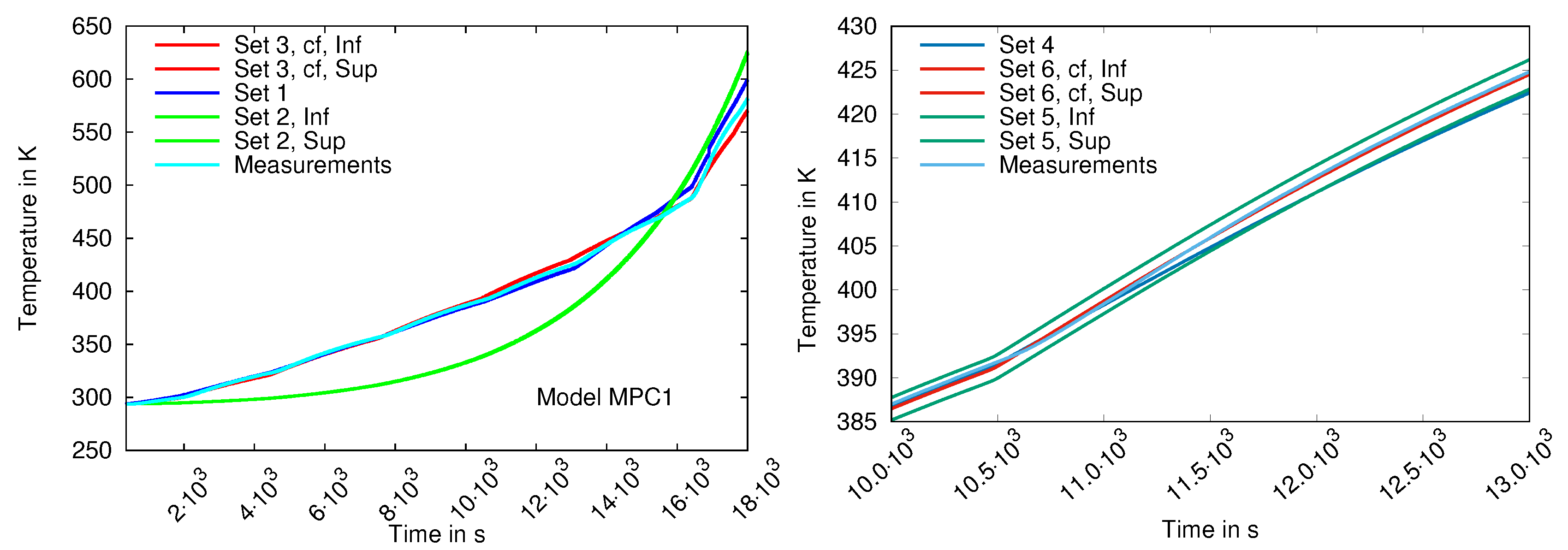
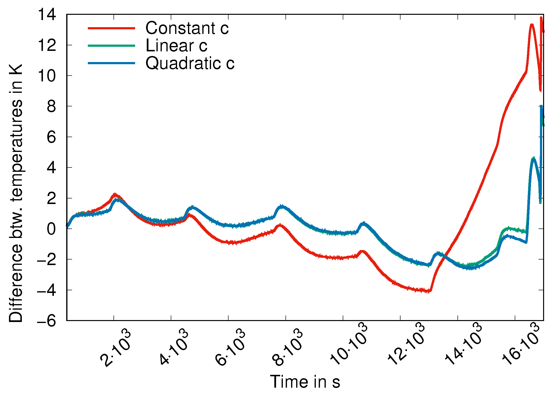
A comparison of simulated temperatures delivered by MPQ1, MPL1 and MPC1 in Figure 3 shows that the model with linear heat capacities has the best accuracy (cf. also

Table 3. Results for MPC1/MPL1 under different conditions. Results for MPQ1 as a comparison. WT1 is the wall time for the optimisation, WT2 for the simulation. The parameter identification using the closed form solution and IPOPT have not been carried out yet for MPL1 due to reasons explained in Section 3.2, therefore “n.d” for Set 6 means “not done”. Times in MATLAB are given only once as a reference.

Set	Model/Setting	Accuracy e	WT 1	WT 2	Degree
1	MPC1/S-MATLAB	4.8255 K	–	–	C3−
2	MPC1/S-VERICELL(i.b)	35.595 K	39 s	348 s	C2−
3	MPC1/S-VERICELL(i.a)	3.5259 K	636 s	<1 s	C2−
4	MPL1/S-MATLAB	2.1260 K	–	–	C3−
5	MPL1/S-VERICELL(i.b)	0.5310 K	95 s	232 s	C2−
6	MPL1/S-VERICELL(i.a)	n.d.	n.d.	<1 s	C2−
7	MPQ1/S-MATLAB	2.1641 K	≈18 h	≈1800 s	C3−

). The simulated and measured temperatures themselves are shown in Figure 4. Surprisingly, the MPL1 simulation results are even better than those of MPQ1 (which are obtained at higher computing times). Generally, the optimisation in two runs and with measurements for the preheaters delivered better parameter sets for MPC1 than the optimisation with the weighted sum in Equation (17). This is the reason for the large difference between measured and simulated data for the option “Set 2” in Figure 4, left. However, the best parameter set for MPC1 is obtained by IPOPT relying on the exact solution (Variant (i.a), Set 3). The computing times are high in this case because we used IPOPT with the exact Hessian matrix obtained by (exact) algorithmic differentiation. None of the computed parameter sets using MPC1 could be proved to be consistent with respect to the condition in Equation (3) ($c_i=15$). For MPL1, the accuracy is better than that for MPC1, and the computing times are comparable.

Note that the simulation times (wall time 2) under S-VERICELL in Table 3 are given for the verified, interval-based solver VNODE-LP and not just for the normal floating point algorithm (as, for example, in Line 7). Generally, we use wall clock times as computing times (if available) in Table 3 since they give a general idea about the actual amount of elapsed time. The times are provided only as a reference since we compare between MATLAB and C++ on different computers. Besides, values of exact derivatives are computed in parallel in UniVerMeC, which explains short wall times for optimisation for Sets 2 and 5 in Table 3.

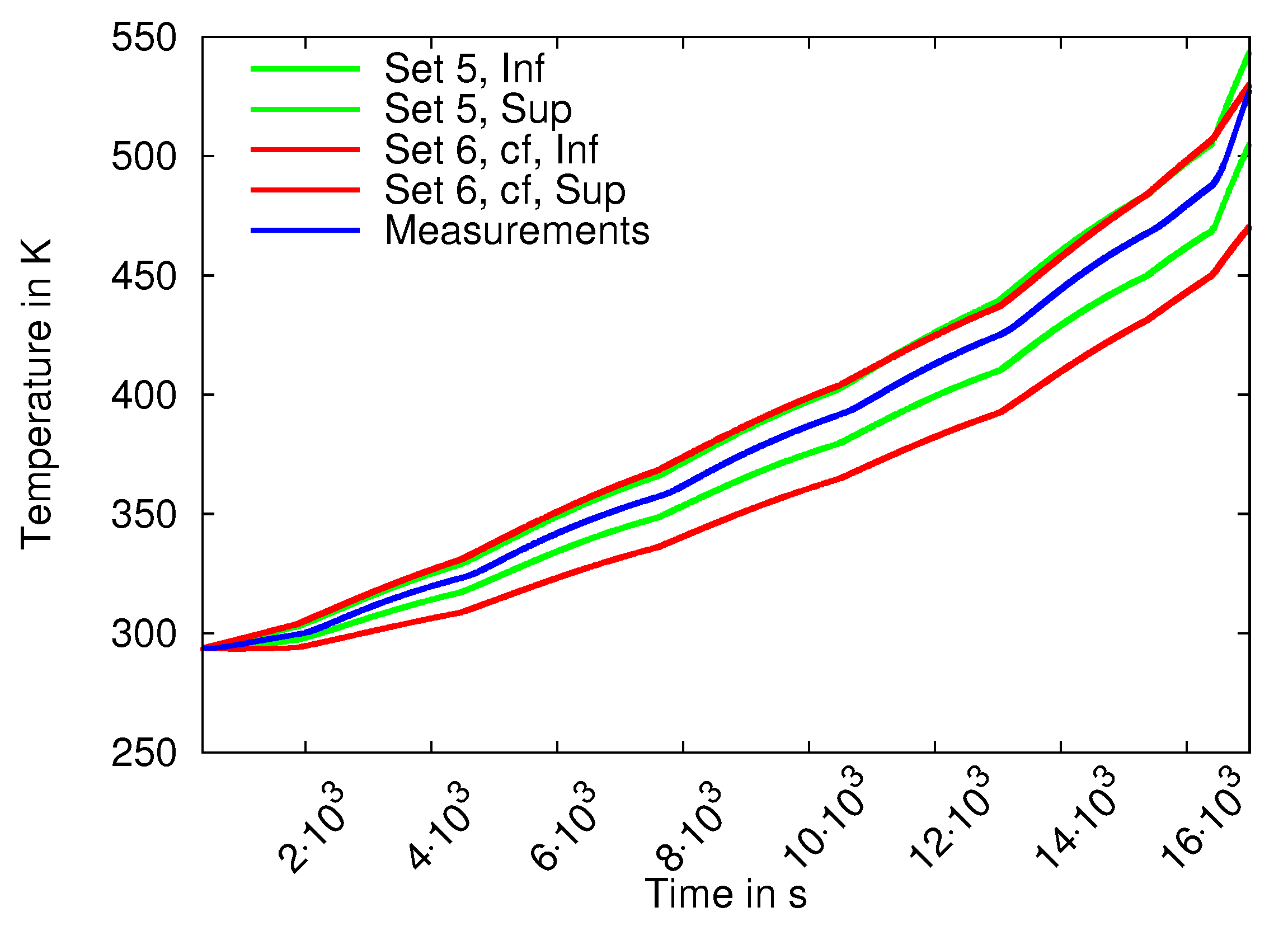
In [10], we showed that introducing uncertainty into MPC1 did not allow us to cover measured data well. For example, the option “Set 2” lead to large overestimation of the true solution set. In Figure 5, we show the results of simulations for MPL1 with $1\%$ uncertainty in all parameters for parameter sets computed by Variant 5 from Table 3. The closed-form-based Variant 6 cannot handle uncertainty very well. Only the uncertainty of $5\times {10}^{-6}\%$ leads to meaningful results for Set 6 with nominal parameters as in Set 4. However, we see in both cases that the solution sets cover the measured data very well. Sets in Variant 5 are not prone to much overestimation.

Overall we can say that the availability of the exact solution improved the quality of the identified parameters. However, the enclosures obtained with uncertainties in parameters were better if VNODE-LP was employed than if we used the closed-form expressions given by Formulas from Section 3. The reason is that the dependency problem in the closed-form might lead to high overestimation for interval arithmetic. This is the case, for example, if ${\alpha }_i$ is identified as negative for the model MPC1. However, the CPU times are better. To improve the quality of enclosures here, we plan to use Taylor models in the future (also for the evaluation of the goal function during parameter identification).

5. Conclusions

In this paper, we showed how modelling possibilities for SOFC systems can be analysed using the process-oriented V&V procedure. Additionally, we pointed out two possibilities to simplify complicated SOFC models in such a way as for them to have closed-form solutions. We studied the models with constant and linear heat capacities and one volume element for the temperature extensively. The overall verification degree of C2− could be attained. The simulations in UniVerMeC were carried out in a verified way, preventing numerical errors. A good parameter set was identified using IPOPT and the exact solution for MPC1. However, this set was still not as good as the parameter set identified with the help of the original, more complicated model with quadratically approximated heat capacities. Overall, the simplified model described the measured data well enough, even though none of the computed parameter sets for MPC1 could be proven to be consistent with respect to the given conditions. The difference between closed-form (i.a) and Euler approximation-based (i.b) versions for MPC1 was dramatic, the former allowing us to identify a much better parameter set. Especially in the context of nonlinear model predictive control, such models can be used in temperature areas with small error ranges in a real-time setting, which we plan to study in the future.

An interesting observation was that the best parameter set sofar (even compared to the usual, non-simplified case) was identified using the model with linearly approximated heat capacities MPL1. In this paper, we confirmed for the one-dimensional temperature model that that kind of simplification was very promising. We simulated that model under $1\%$ uncertainty in parameters and showed that a complete coverage of measured data in case of MPL1 could be achieved. However, the parameter identification using the derived closed-form solution remains a topic for the further research. We also plan to use the “verified approximation” (i.b) version of this model for higher dimensions in our future work.

Models relying on ODEs using more than one volume element to describe the temperature of the SOFC stack are necessary for better control of the temperature inside the stack. However, they cannot be solved analytically in general for non-constant heat capacities. Even in the “constant” case, the exact solutions might get too complicated to bring any measurable quality improvement. However, simulations with linearized or constant approximations to heat capacities might reduce overall computing times for higher-dimensional models, which is also a topic for our future work.