Performance Analysis of Four Decomposition-Ensemble Models for One-Day-Ahead Agricultural Commodity Futures Price Forecasting

Abstract

Agricultural commodity futures prices play a significant role in the change tendency of these spot prices and the supply–demand relationship of global agricultural product markets. Due to the nonlinear and nonstationary nature of this kind of time series data, it is inevitable for price forecasting research to take this nature into consideration. Therefore, we aim to enrich the existing research literature and offer a new way of thinking about forecasting agricultural commodity futures prices, so that four hybrid models are proposed based on the back propagation neural network (BPNN) optimized by the particle swarm optimization (PSO) algorithm and four decomposition methods: empirical mode decomposition (EMD), wavelet packet transform (WPT), intrinsic time-scale decomposition (ITD) and variational mode decomposition (VMD). In order to verify the applicability and validity of these hybrid models, we select three futures prices of wheat, corn and soybean to conduct the experiment. The experimental results show that (1) all the hybrid models combined with decomposition technique have a better performance than the single PSO–BPNN model; (2) VMD contributes the most in improving the forecasting ability of the PSO–BPNN model, while WPT ranks second; (3) ITD performs better than EMD in both cases of corn and soybean; and (4) the proposed models perform well in the forecasting of agricultural commodity futures prices.

1. Introduction

Regarding commodity markets, the entirety of last year was unforgettable and catastrophic because, with the most diminution in crude oil and iron ore, the Bloomberg Commodity Index, composed of 22 international commodities’ futures prices, including six agricultural commodities, has dropped over 24 percent compared with 2014, which is the third consecutive annual loss and the largest annual decline since the financial crisis in 2008. Serving as an important composition of international commodity markets, agricultural commodity futures prices have actually begun to show a distinct downward tendency since 2013. Generally speaking, agricultural commodity prices and the relationship between supply and demand mutually affect one another to a large extent. However, over the past few years, although agricultural commodity markets have experienced relatively serious weather disruptions such as El Niño and a potential La Niña, the growth rate of supply of the majority of agricultural commodities, especially food grain, has exceeded the rate of demand, which to some extent makes these prices recover modestly or even keep falling.

Regarded as the three leading world economies, the United States is a large consumer of corn, the European Union is the same for wheat, and China is a large importer of soybean, which means that these agricultural commodities play an important role in these countries’ social economy and daily life. These kinds of food grain market data, including price data, are vital for any future agriculture development project because there is strong mutual influence between price and potential supply and demand, as well as for distribution channels of food grain and the economics of agriculture [1]. According to the futures price discovery mechanism and the high sensitivity of macroeconomic situations or policies, they can conduct price information to the spot markets in advance. Thus, the price forecasting of these futures prices is expected to not only reduce the uncertainty and control the risk in agricultural commodity markets, but can also be applied to identify and make appropriate and sustainable food grain policies for the government.

A large body of the existing literature, however, has explored the related research of agricultural commodities, such as yield forecasting [2,3,4], price co-movement or volatility [5,6,7,8,9,10,11,12,13,14], spot price forecasting [1,15], market efficiency [16], and trade policy responses [17], instead of investigating the predictability of agricultural commodity futures prices [18,19,20,21]. Fortunately, in past decades, abundant research achievements have been made in forecasting a wide range of time series, some of which can be used for reference to solve the problem of forecasting agricultural commodity futures prices because of the common features of the time series.

Building models to forecast time series is always a complicated, difficult but attractive challenge for scholars, which contributes to the large number of research achievements accumulated. Initially, scholars focus on using single models based on only one linear or nonlinear forecasting method to forecast time series. Some researchers make efforts to apply traditional statistic approaches such as the vector auto-regression (VAR) model, vector error correction models (VECM), autoregressive integrated moving average (ARIMA), and generalized autoregressive conditional heteroskedasticity (GARCH) to discuss price data series. For instance, Mayr and Ulbricht [22] employ VAR models to forecast GDP based on the log-transforming data from four countries, namely the USA, Japan, Germany and the United Kingdom in a certain period. Kuo [23] uses data from the Taiwanese market to compare the relative forecasting performance of VECM with the VAR as well as the ordinary least square (OLS) and random walk (RW) applied in past literature. ARIMA is utilized by Sen et al. to forecast the energy consumption and greenhouse gas (GHG) emission of an Indian pig iron manufacturing organization, and two best fitted ARIMA models are determined respectively [24]. The GARCH model is initially used to forecast the Chicago Board Options Exchange (CBOE) volatility index (VIX) by Liu et al. [25]. With the fast development of artificial intelligence (AI) techniques, artificial neural network (ANN) and machine learning (ML) are gaining increasing focus on forecasting time series data, aiming to overcome the limitations of traditional statistic methods; for instance, they are unable to easily capture nonlinear patterns. Hsieh et al. [26] propose the back-propagation neural network (BPNN), integrating with design of experiment (DOE) and the Taguchi method, to further optimize the prediction accuracy. According to Yan and Chowdhury [27], a multiple support vector machine (SVM) is presented to study the forecasting of the mid-term electricity market clearing price (MCP). In addition, the application of optimization algorithms [28,29,30,31,32,33,34], such as particle swarm optimization (PSO), artificial bee colony (ABC), fruit fly optimization algorithm (FOA), ant colony optimization (ACO) and differential evolution (DE), has improved the forecasting performance and slowed processing speed of the AI techniques.

However, price time series in the real world rarely appears in a linear or nonlinear pattern solely, but usually covers both patterns, so that hybrid models emerge, combining several single models systematically [35], which can simultaneously handle linear and nonlinear patterns [21]. A hybrid methodology that exploits the unique strength of the ARIMA and the SVM is proposed by Pai and Lin [36] to tackle stock prices forecasting problems, which gains very promising results. Since then, it has not been difficult to find that great research efforts have been made to explore the “linear and nonlinear” modelling framework used in time series prediction. For example, Khashei and Bijari [37] present a novel hybridization of ANN and ARIMA to forecast three well-known data sets, namely the Wolf’s sunspot data, the Canadian Iynx data and the British pound/US dollar exchange rate. A hybrid model combining VECM and multi-output support vector regression (VECM-MSVR), which is expert in capturing the linear and nonlinear patterns, is devised to make interval forecasting of agricultural commodity futures prices [21].

Undoubtedly, past literature provides many effective and reasonable models to forecast time series and improve the forecasting performance to some extent. However, these models often cannot thoroughly handle the non-stationarity of random and irregular time series. Thus, based on decomposition techniques such as the wavelet transform (WT) family methods, the empirical mode decomposition (EMD) family approaches, and the variational mode decomposition (VMD) method, a promising concept of “decomposition and ensemble” is developed [35] to enhance the forecasting ability of the existing models. For example, four real-world time series are predicted through a novel combination of ARIMA and ANN models based on the discrete wavelet transform (DWT) decomposition technique [38]. Wang et al. [39] build a novel least square support vector machine (LSSVM) optimized by PSO based on simulated annealing (PSOSA) (abbreviated as PSOSA-LSSVM) to forecast wind speed data preprocessed by the wavelet packet transform (WPT). According to Yu et al. [40], two kinds of crude oil spot prices, the West Texas Intermediate (WTI) and the Brent, are predicted by the EMD-based neural network. As for intraday stock prices forecasting, Lahmiri [31] develops a hybrid VMD–PSO–BPNN predictive model that finally shows the superiority over the benchmark model, namely a PSO–BPNN model. Beyond that, many other decomposition-based forecasting models [41,42,43,44,45,46] have been proposed, which greatly enriches the empirical achievement of time series predictive models, on the basis of the “decomposition and ensemble” framework, and further improves time series forecasting performance.

It is evident that the “decomposition and ensemble” modelling framework has been recently well-established to forecast time series in many fields, such as commodity prices, energy demand or consumption, wind speed, etc. Still, however, no research exists on forecasting agricultural commodity futures prices using this kind of promising framework. Thus, in this paper, we aim to put forward four new hybrid models, based on the “decomposition and ensemble” framework, which are utilized to forecast three agricultural commodity futures prices; namely wheat, corn and soybean. Specifically, these four models are based on the PSO–BPNN combined with four different decomposition techniques, namely the WPT, EMD, VMD and intrinsic time-scale decomposition (ITD) [47], respectively, generating four models, namely the WPT–PSO–BPNN model, the EMD–PSO–BPNN model, the VMD–PSO–BPNN model and the ITD–PSO–BPNN model. Therefore, the data pretreatment effect of different decomposition techniques is horizontally compared. Meanwhile, the decomposition techniques we select include more types, which can contribute to more comprehensive comparison in contrast to Liu et al. [48].

The reminder of this paper is organized as follows. Section 2 introduces the methodologies applied in this paper, containing the decomposition methods, the PSO algorithm, the BPNN, and the proposed hybrid models. Research design is concretely described in Section 3. Then, Section 4 shows results and analysis of the three study cases. Finally, conclusions of this paper are given in Section 5.

2. Methodology

This section presents the introduction of the proposed methodology we use to forecast the agricultural commodity futures prices, namely wheat, corn and soybean, which includes decomposition methods, back propagation neural network, particle swarm optimization algorithm, and the proposed hybrid models based on these approaches.

2.1. Decomposition Methods

Recently, signal decomposition techniques have been attracting increasing attention in many research fields, including time series preprocessing. In this part, the four representative decomposition approaches are described as below.

2.1.1. Empirical Mode Decomposition

Serving as an adaptive and highly efficient decomposition approach, the empirical mode decomposition (EMD) is proposed by Huang et al. [49] to analyze nonlinear and nonstationary time series, which solves the problem that the full description of the frequency content cannot be obtained by single Hilbert transform. Certainly, this decomposition method is based on some assumptions: (1) the original signal at least contains one maximum and one minimum; (2) the characteristic time scale is defined by the time lapse between the extrema; and (3) only when the data totally lack extrema but contain inflection points can it be differentiated once or more times to reveal the extrema. Through the EMD method, the time series data can be converted into a finite and often small number of intrinsic mode functions (IMFs). As for the original data $X_t$, the sifting process of EMD is illustrated as follows [49]:

• Apply a cubic spline line to connecting all the local maxima and minima to produce the upper envelope and lower envelope, respectively.
• Calculate the mean of upper and lower envelope, $m_1$, which then is used to obtain the first component, $h_1$, as shown in the following equation:

  $$X_t-m_1=h_1$$

  (1)
• Check whether the $h_1$ is an IMF, which satisfies two conditions (see [49] for detail), or not. If not, treat it as the original data and repeat step 1 and 2 $k$ times until $h_{1k}$ is an IMF, designated as $c_1$, that is

  $$h_{1\left(k-1\right)}-m_{1k}=h_{1k}=c_1$$

  (2)

  and the residue,$r_1$, is denoted as:

  $$X_t-c_1=r_1$$

  (3)
• Regard $r_1$ as the new original data and tackled with the same sifting process presented above in order to further extract the information of longer period components contained in it. Repeat this process until the last residue becomes a monotonic function from which no more IMF can be extracted. The results are then shown as below:

  $$r_1-c_2=r_2,r_2-c_3=r_3,\dots ,r_{n-1}-c_n=r_n$$

  (4)
• Sum up Equations (3) and (4), and the ultimate decomposition results of EMD are obtained as follows:

  $$X_t={\displaystyle \sum _{i=1}^n{c}_i}+r_n$$

  (5)

  where $c_i$ is the ith component, and $r_n$ is the final residue.

2.1.2. Wavelet Packet Transform

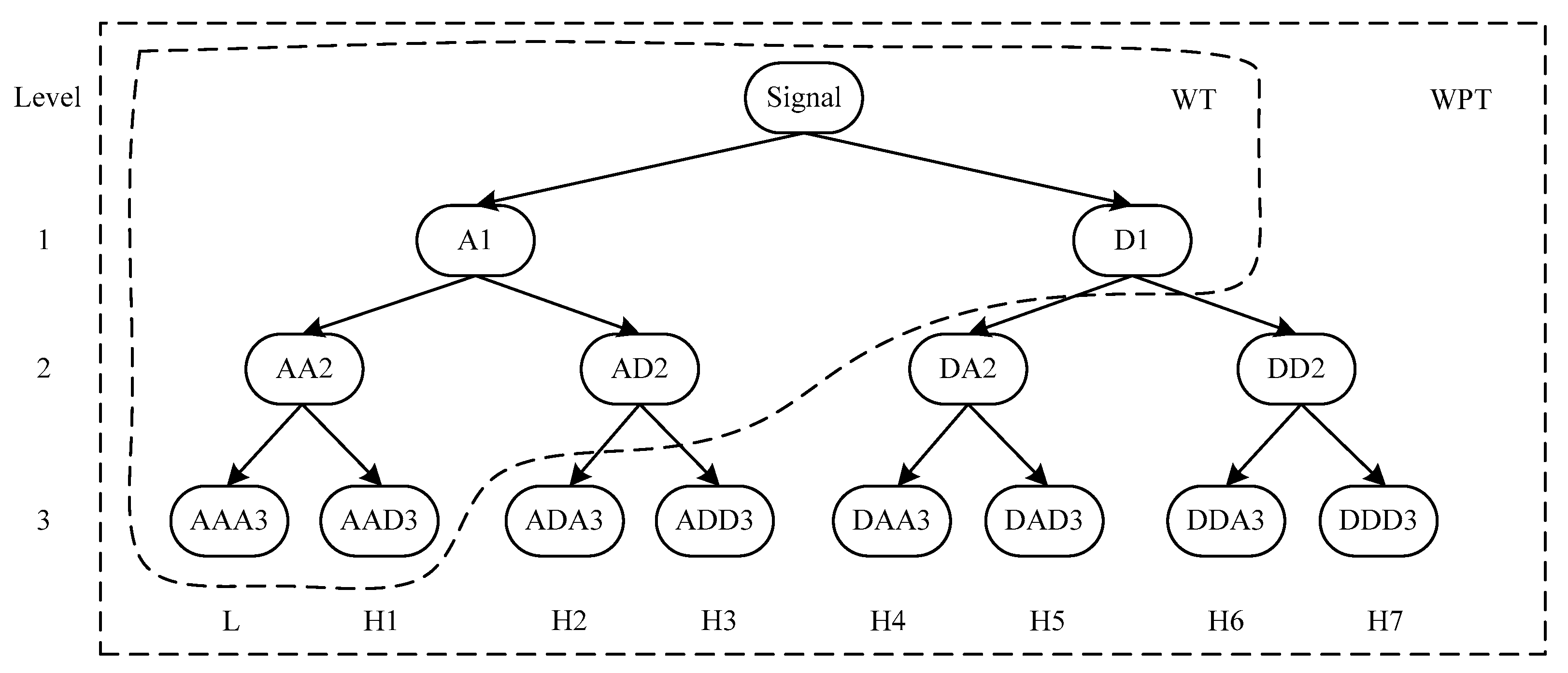
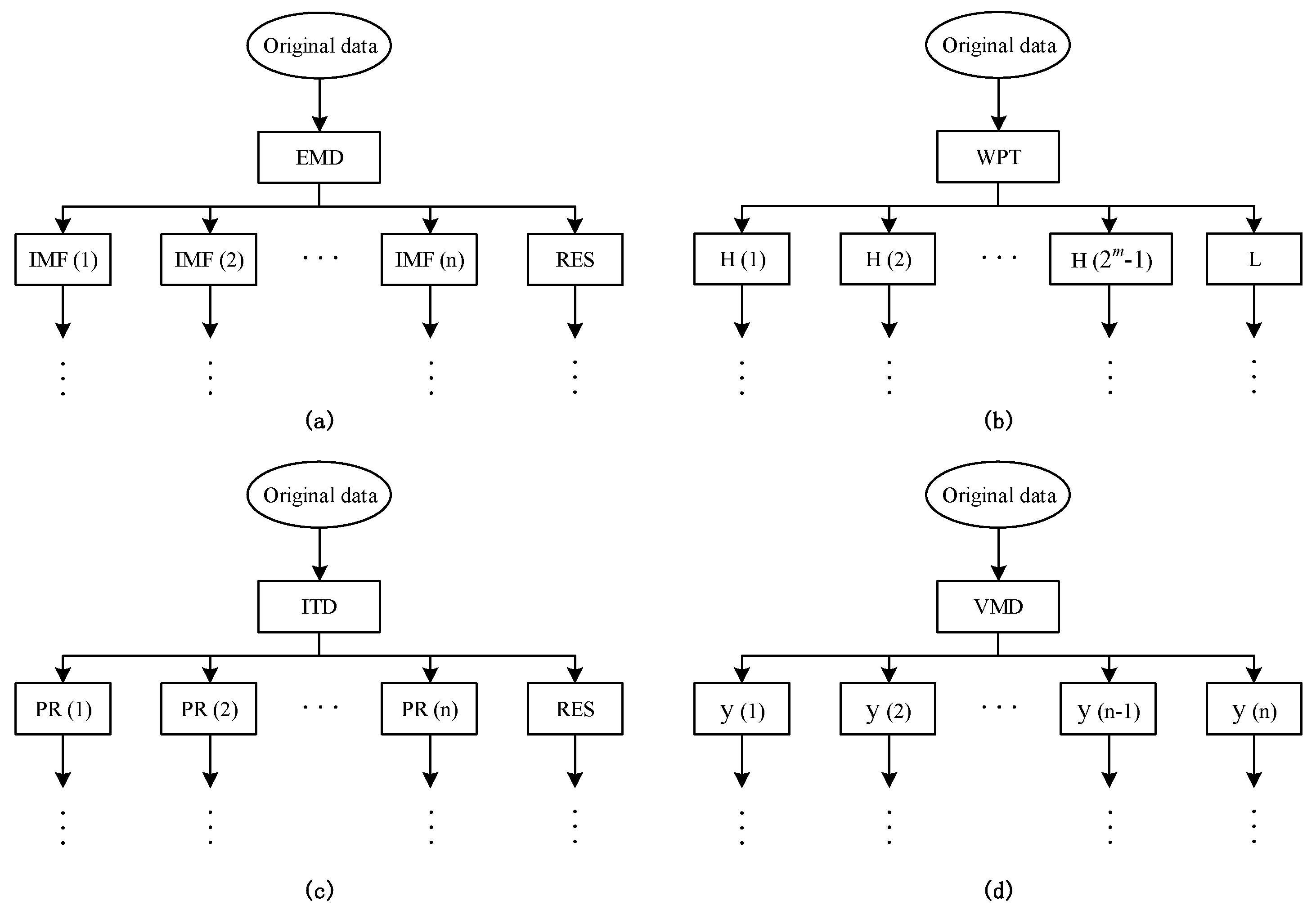
The wavelet transform (WT), first proposed by Mallat [50] to study data compression in image coding, texture discrimination and fractal analysis, is a multi-scale signal processing method with good time-frequency localization features. However, this approach simply decomposes the low frequency sub-series of the original signal and ignores the analysis of the sub-series with high frequencies, which makes it more suitable to process nonstationary and instantaneous signals instead of gradually-changed signals. Thus, the wavelet packet transform (WPT) was developed, based on the WT, to overcome this limitation. Similar to the WT, the WPT decomposes the original signal into a low frequency coefficient (called approximation) and a set of high frequency coefficients (called details). By contrast, the WPT can further convert each detail into another approximation and another detail. 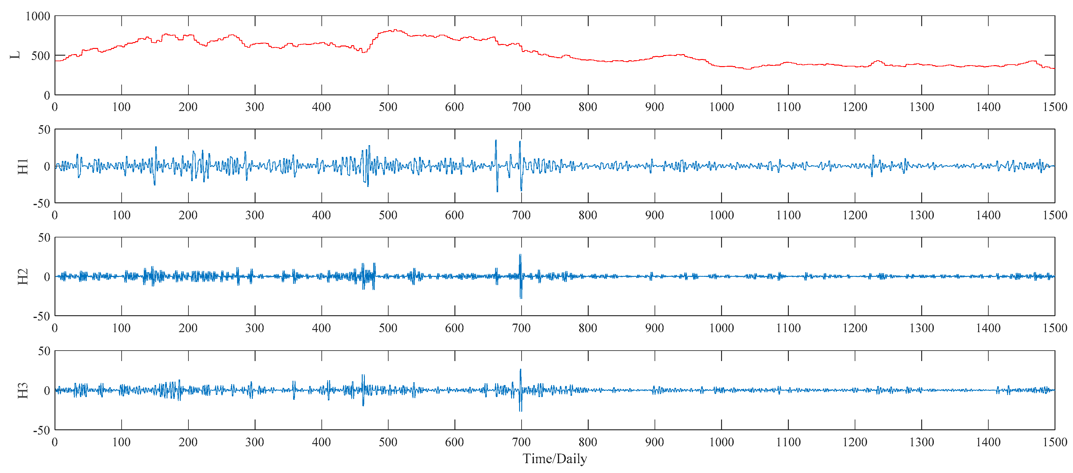Taking three decomposition level as an example, we illustrate the comparison of the decomposition trees of WT and WPT in Figure 1. As to the WPT, the final decomposition results of three level cover one approximation, L, and seven details, denoted by the H1, H2, …, H7, respectively.

2.1.3. Intrinsic Time-Scale Decomposition

According to Frei and Osorio [47], the intrinsic time-scale decomposition (ITD) is developed for the efficient and precise time–frequency–energy (TFE) analysis of signals. Based on this approach, a nonlinear or nonstationary signal can be decomposed in to a set of proper rotation (PR) components and a monotonic trend, namely a residual signal. Given a signal $X_t$, the decomposition process of ITD algorithm is illustrated as follows:

• An operator, $\xi$, which extracts a baseline signal from $X_t$, is defined. More specifically, $X_t$ can be decomposed as:

  $$X_t=\xi X_t+\left(1-\xi \right)X_t=L_t+H_t$$

  (6)

  where $L_t=\xi X_t$ and $H_t=\left(1-\xi \right)X_t$ represent the baseline signal and a proper rotation respectively.
• Suppose that $\left\{X_t,t\ge 0\right\}$ is a real-valued signal, while the local extrema of $X_t$ is defined as $\left\{{\tau }_k,k=1,2,\dots \right\}$, and let ${\tau }_0$ be equal to zero. For convenience, $X\left({\tau }_k\right)$ and $L\left({\tau }_k\right)$ are abbreviated as $X_k$ and $L_k$, respectively.${\tau }_k$ is taken as the right endpoint of the interval, containing extrema due to the neighboring signal fluctuation, where $X_t$ is constant. Meanwhile, suppose that $L_t$ and $H_t$ have been defined on the interval, $\left[0,{\tau }_k\right]$, and that $X_t$ is available for $t \in \left[0,{\tau }_{k+2}\right]$. Thus, a (piece-wise linear) baseline-extracting operator, $\xi$, is defined on the interval $\left({\tau }_k,{\tau }_{k+1}\right]$ between successive extrema as follows:

  $$\xi X_t=L_t=L_k+\left(\frac{L_{k+1}-L_k}{X_{k+1}+X_k}\right)\left(X_t-X_k\right)\hspace{1em}s.t.\hspace{1em}t\in \left({\tau }_k,{\tau }_{k+1}\right]$$

  (7)

  where

  $$L_{k+1}=\alpha \left[X_k+\left(\frac{{\tau }_{k+1}-{\tau }_k}{{\tau }_{k+2}-{\tau }_k}\right)\left(X_{k+2}-X_k\right)\right]+\left(1-\alpha \right)X_{k+1}$$

  (8)

  and the parameter, $\alpha \in \left(0,1\right)$, is usually determined as 0.5.
• After defining the baseline signal based on Equations (7) and (8), it is possible to define the residual, proper-rotation-extracting operator, $\psi$, as:

  $$\psi X_t\equiv \left(1-\xi \right)X_t=H_t=X_t-L_t$$

  (9)

2.1.4. Variational Mode Decomposition

Variational mode decomposition (VMD) [51], a newly non-recursive signal processing technique, is utilized to adaptively decompose a real valued signal into a discrete number of band-limited sub-signals, namely the modes $y_k$, having specific sparsity properties. Each mode decomposed by the VMD approach can be compressed around a center pulsation $w_k$, which is determined along with the decomposition process. To estimate the bandwidth of each mode, the following procedures should be considered: (1) as to each mode $y_k$, applying the Hilbert transform to calculate the associated analytic signal so that a unilateral frequency spectrum can be obtained; (2) mixing with an exponential tuned to the respective estimated center frequency in order to shift the mode’s frequency spectrum to baseband; and (3) estimating the bandwidth for each mode $y_k$ by using the H¹ Gaussian smoothness of the demodulated signal. Thus, the constrained variational problem can be presented as follows:

$$\underset{\left\{y_k\right\},\left\{w_k\right\}}{\min }\left\{{\displaystyle \sum _{k=1}^{\mathrm{K}}{\Vert {\partial }_t\left[\left(\delta \left(t\right)+\frac{j}{\pi t}\right)\otimes y_k\left(t\right)\right]e^{-j{w}_{k}t}\Vert }_2^2}\right\}\hspace{1em}s.t.\hspace{1em}{\displaystyle \sum _{k=1}^K{y}_k}=f\left(t\right)$$

(10)

where $f\left(t\right)$ is the original main signal, $y_k$ is the kth component of the original signal; $w_k$, $\partial \left(t\right)$ and $\otimes$ represent center frequency of $y_k$, the Dirac distribution and convolution operator, respectively; k denotes the number of modes, while t is time script.

Taking both penalty term and Lagrangian multipliers $\lambda$ into consideration, the above constrained problem can be converted into an unconstrained one that can be addressed more easily, which is shown as follows:

$$\begin{array}{l}L\left(\left\{y_k\right\},\left\{w_k\right\},\lambda \right)=\\ \alpha {\displaystyle \sum _{k=1}^K{\Vert {\partial }_t\left[\left(\delta \left(t\right)+\frac{j}{\pi t}\right)\otimes y_k\left(t\right)\right]e^{-j{w}_{k}t}\Vert }_2^2+{\Vert f\left(t\right)-{\displaystyle \sum _{k=1}^K{y}_k\left(t\right)}\Vert }_2^2+\langle \lambda \left(t\right),f\left(t\right)-{\displaystyle \sum _{k=1}^K{y}_k\left(t\right)}\rangle }\end{array}$$

(11)

where $\alpha$ represents the balancing parameter of the data fidelity constraint.

The augmented Lagrangian L is determined in Equation (11) and its saddle point in a sequence of iterative sub-optimizations can be found through using the alternate direction method of multipliers (ADMM). According to this ADMM optimization method, it is assumed that updating $y_k$ and $w_k$ in two directions helps to realize the analysis process of the VMD. The complete and detailed procedures of this algorithm are available in [51]. Consequently, solutions for $y_k$ and $w_k$ are described as follows [51]:

$${\widehat{y}}_k^{n+1}=\frac{\widehat{f}\left(w\right)-{\displaystyle \sum _{i\ne k}{\widehat{y}}_i\left(w\right)+\frac{\widehat{\lambda }\left(w\right)}{2}}}{1+2\alpha {\left(w-w_k\right)}^2}$$

(12)

$$w_k^{n+1}=\frac{{{\displaystyle {\int }_0^{\infty }w\left|{\widehat{y}}_k^{n+1}\left(w\right)\right|}}^{2}dw}{{{\displaystyle {\int }_0^{\infty }\left|{\widehat{y}}_k^{n+1}\left(w\right)\right|}}^{2}dw}$$

(13)

where $\widehat{f}\left(w\right)$, ${\widehat{y}}_i\left(w\right)$, $\widehat{\lambda }\left(w\right)$ and ${\widehat{y}}_k^{n+1}\left(w\right)$ denote the Fourier transforms of $f\left(t\right)$, $y_i\left(t\right)$, $\lambda \left(t\right)$ and $y_k^{n+1}\left(t\right)$ respectively, while n represents the number of iterations.

2.2. Back Propagation Neural Network

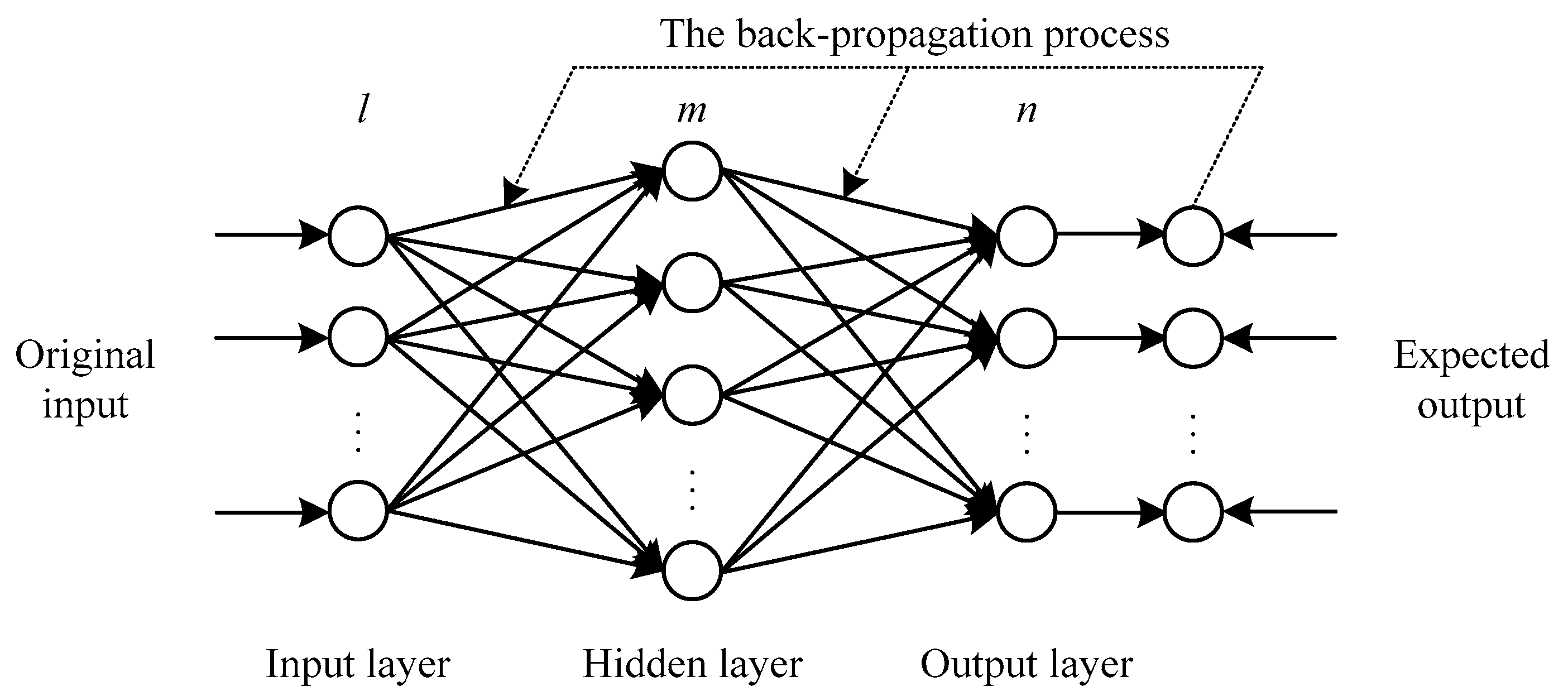
A back propagation neural network (BPNN) is a typical kind of feed-forward artificial neural network based on the back propagation algorithm, which is widely applied in many research areas. Compared with conventional statistic methods, one remarkable advantage of the BPNN is that it can approximate any nonlinear continuous function up to any desired accuracy. Generally speaking, a BPNN consists of one input layer, one or more hidden layer and one output layer. In our study, the number of the hidden layers is determined as one, based on Khandelwal et al. [38], so that a standard three-layer $l\times m\times n$ BPNN structure is developed, as shown in Figure 2. More specifically, the mathematical representation of its training process can be described as follows:

• The output of the hidden layer nodes, $y_j^h$, can be calculated as:

  $$y_j^h=\delta \left({\displaystyle \sum _{i=1}^l{w}_{ji}{x}_i+b_j}\right)$$

  (14)

  where $w_{ji}$ is the connection weight from the ith input node to jth hidden node, $x_i$ means the ith input data, $b_j$ represents the bias of jth hidden neuron, and $\delta (·)$ denotes the nonlinear transfer function of the hidden layer, which usually is a sigmoid function.
• Then, the output of this neural network, $y_k^o$, can be obtained by:

  $$y_k^o=\rho \left({\displaystyle \sum _{j=1}^m{w}_{kj}{y}_j^h+b_k}\right)$$

  (15)

  where $w_{kj}$ represents the weight connecting jth hidden node to kth output node, $b_k$ is the bias of the kth output neuron, and $\rho (·)$ means the output layer’s transfer function, which is a linear one by default.
• The goal of BPNN is to minimize the error E, namely the mean square error (MSE) by default, which can be measured by:

  $$E=\frac{1}{N}{\displaystyle \sum _{t=1}^N{\displaystyle \sum _{k=1}^n\left(y_k-y_k^o\right)}}{}^2$$

  (16)

  where N is the number of input sample, $y_k$ denotes the kth expected output data.

2.3. Particle Swarm Optimization Algorithm

Particle swarm optimization (PSO) is an optimization algorithm based on swarm intelligence put forward by Kennedy and Eberhart in 1995; the basic principle is derived from the artificial life and the predation behavior of groups of birds. In the population, every particle represents a potential solution, and every particle has a fitness degree value, which is determined by the objective function. The movement direction and distance of the particle depend on the speed of the particle, which is adjusted dynamically according to itself and the movement experience of other particles, and the individual obtains optimal solution in the solution space.

In the d dimension space composed of n particles, express the speed of particle i as $v_i={(v_{i1},v_{i2},\cdots ,v_{id})}^T$, express the position as $x_i={(x_{i1},x_{i2},\cdots ,x_{id})}^T,i=1,2,\dots ,n$, pbest is the optimal position that particle i has crossed, gbest is the optimal position that the population has crossed; in every iteration, particles update their speed and position by individual extremum pbest and global extremum gbest, update formulas are shown as follows:

$$v_{id}^{k+1}=\omega v_{id}^k+c_1{r}_1(pbes{t}_{id}^k-x_{id}^k)+c_2{r}_2(gbes{t}_{id}^k-x_{id}^k)$$

(17)

$$x_{id}^{k+1}=x_{id}^k+v_{id}^{k+1}$$

(18)

where $v_{id}^k$ is the speed of particle i in the kth iteration and dth dimension; $\omega$ is inertia weight; $c_1$ and $c_2$ are are acceleration factor, $r_1$ and $r_2$ are the random numbers ranging from 0 to 1.

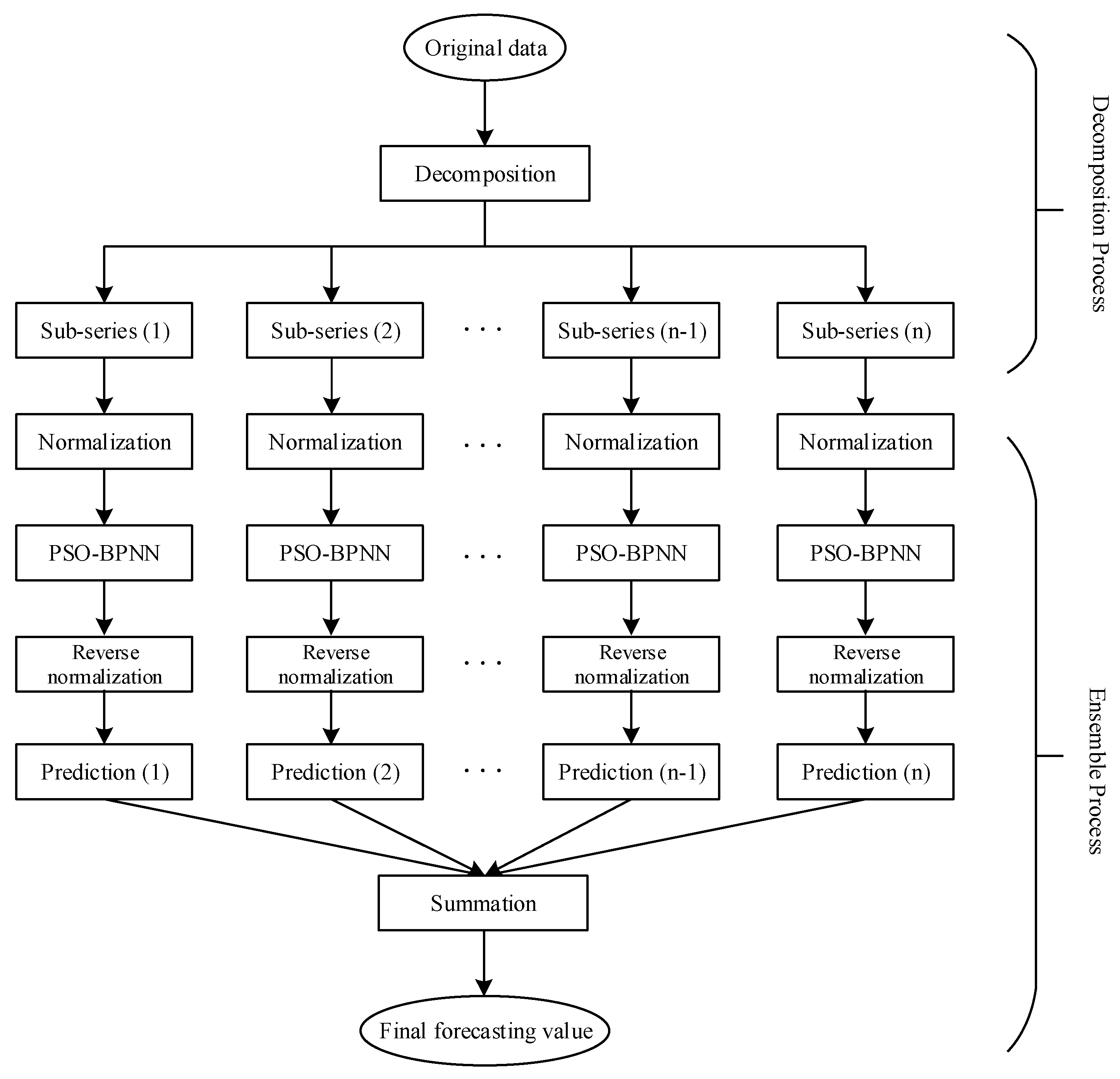
2.4. The Proposed Hybrid Models

In this subsection, the four proposed hybrid models, which contains the WPT–PSO–BPNN model, the EMD–PSO–BPNN model, the ITD–PSO–BPNN model and the VMD–PSO–BPNN model, are developed on the basis of the methodology mentioned above to forecast the day-ahead prices of the wheat, corn and soybean futures which will be described concretely in the next section; the basic structure of these models is given in Figure 3.

Weight and threshold are two important parameters in the BPNN which would have an influence on the forecasting accuracy. The PSO algorithm, with its advantages of fast rate and high efficiency, is regarded as a widespread optimization tool based on the swarm intelligence. Therefore, we apply this approach in optimizing these two parameters. Furthermore, agricultural commodity futures prices are nonlinear and nonstationary time series data with relatively obvious volatility, which can be handled through the decomposition techniques to some extent. Thus, the hybrid models are established. It is necessary to note that, in our study, all components decomposed are normalized into the range of [0, 1] using linear transference method before entering the next step, for better convergence of the BPNN. Certainly, the output data should be rescaled back by reversing the normalization in order to compute the forecasting accuracy on the basis of the original scale of the data. All calculating and modelling processes involved in this paper are realized in MATLAB R2015b.

3. Research Design

This section describes details about the research design on data selection and description, data preprocessing, forecasting performance evaluation criteria and experimental procedure.

3.1. Data Selection and Description

As mentioned in the first section, in order to make comparison of the forecasting performance among different models, our study chooses three agricultural commodity futures prices—namely the wheat, corn and soybean—to conduct empirical research. The original data of these three futures prices are obtained from the Chicago Board of Trade (CBOT), which is available on the CME Group’s website (http://www.cmegroup.com/). The reasons why we take these three agricultural commodity futures prices as research objects are as follows: (1) CME Group is the world’s leading and most diverse derivatives marketplace, and how its futures prices change usually does have a great effect on other countries’ futures markets, which certainly includes wheat, corn and soybean futures; (2) these agricultural commodities feed a large part of the world’s population directly or indirectly [15], which will strengthen the interplay between food grain futures prices and its supply-demand situation to some extent; and (3) corn, wheat and soybean play an extremely important role in the world’s three leading economics which are the United States, the European Union and China, respectively, in the aspect of consuming and importing.

More specifically, we choose these three commodities’ closing prices of continuous futures contracts as sample data in our study, which are daily data with the same sample size (1500 observations) but covering different periods, shown in

Table 1. Period and length of the three futures prices.

Futures	Period	Sample Size	Training Set	Testing Set
Corn	13 August 2010 to 29 July 2016	1500	1200	300
Soybean	10 August 2010 to 29 July 2016	1500	1200	300
Wheat	13 August 2010 to 29 July 2016	1500	1200	300

. Note that the wheat futures explicitly represent the Chicago SRW wheat futures, since its average daily volume (ADV) is larger than other wheat futures based on the CME Group’s leading products reports. Meanwhile, for each sample data of wheat, corn and soybean, the first 1200 observations (80%) are taken as the training set of models proposed above, while the last 20% (300 observations) is treated as the testing set (See Table 1). In the process of forecasting each dataset, the PSO–BPNN is trained by the training set corresponding to the dataset, and after this, the study uses the testing set to evaluate and compare the forecasting performance of all hybrid models presented in this paper.

Figure 4 gives the sequence chart of the daily futures prices of wheat, corn and soybean. It can be seen from this figure that the soybean futures prices keep at a higher level than other two futures during the whole period, while the corn futures prices are a little lower than the prices of wheat in most of this period. Although prices of these three futures differ from each other, they approximately have their movement trend in common. Furthermore, all three futures price time series, which are nonlinear and nonstationary in nature, show the characteristics of relatively large fluctuation, which can help the decomposition methods to well exert the role of data pretreatment.

3.2. Data Preprocessing

One of the key contributions in this study is to establish agricultural commodity futures price forecasting models combined with the four decomposition methods mentioned in Section 2.1, respectively. In this subsection, we will illustrate how to utilize the EMD method, WPT method, ITD method and VMD method to preprocess sample data, respectively.

As for the EMD method, the original time series of each agricultural commodity futures prices can be easily decomposed into a sum of IMFs and a residue, RES. For the specific sample data, the number of components decomposed by EMD is fixed, namely that there is no access to changing the number of decomposition manually in terms of a specific sample data. The process of EMD method is given in Figure 5a.

As for the WPT method, it is worth noting that this method can preset different number of decomposition level manually. For instance, for each m level of decomposition, the WPT approach generates 2^m different set of sub-series, namely 2^m − 1 details represented by H(1), …, H(2^m − 1), and one approximation, L. Figure 5b shows this approach’s process of decomposition.

As for the ITD method, it can decompose the original data into a set of PR components and a residual signal, RES. Different from other three decomposition techniques, it allows researchers to put an upper limit on the number of decomposition, which means the ultimate number is less than or equal to that upper limit. See Figure 5c for the concrete process of the ITD method.

As for the VMD method, the number of modes is able to be changed in the light of the research needs. Therefore, some experiments are conducted in order to select out the best decomposition number for time series forecasting in this study, which is illustrate in Section 4. The decomposition process is presented in Figure 5d.

3.3. Forecasting Performance Evaluation Criteria

In order to verify the validity of the proposed model in this paper, we select three generally adopted error indexes to evaluate the performance of proposed model compared with other models, including mean absolute error (MAE), root mean square error (RMSE) and mean absolute percentage error (MAPE). The paper comprehensively evaluates the forecasting performance by these three methods. The computational equations of these three error methods are given as follows:

$$MAE=\frac{1}{N}{\displaystyle \sum _{t=1}^N\left|\widehat{y}(t)-y(t)\right|}$$

(19)

$$RMSE=\sqrt{\frac{1}{N}{{\displaystyle \sum _{t=1}^N\left(\widehat{y}(t)-y(t)\right)}}^2}$$

(20)

$$MAPE=\frac{1}{N}{\displaystyle \sum _{t=1}^N|\frac{\widehat{y}(t)-y(t)}{y\left(t\right)}}|$$

(21)

where $N$ is the number of the testing sample, $y\left(t\right)$ is the actual data of each dataset, and $\widehat{y}\left(t\right)$ is the forecasting value of the corresponding futures prices data.

3.4. Experimental Procedure

According to Figure 3, it is not difficult to see that our study’s experimental procedure mainly includes four steps: first, for each sample data of wheat, corn and soybean futures, we use EMD, WPT, ITD and VMD to decompose them, respectively, which generates a sum of sub-series; second, we normalize each sub-series by the specified linear transference before entering the forecasting part; third, we input all normalized sub-series into the PSO–BPNN model, obtaining a set of predictions which are treated by reversing the normalization; fourth, we sum up all predictions to get the final forecasting value.

4. Results and Analysis

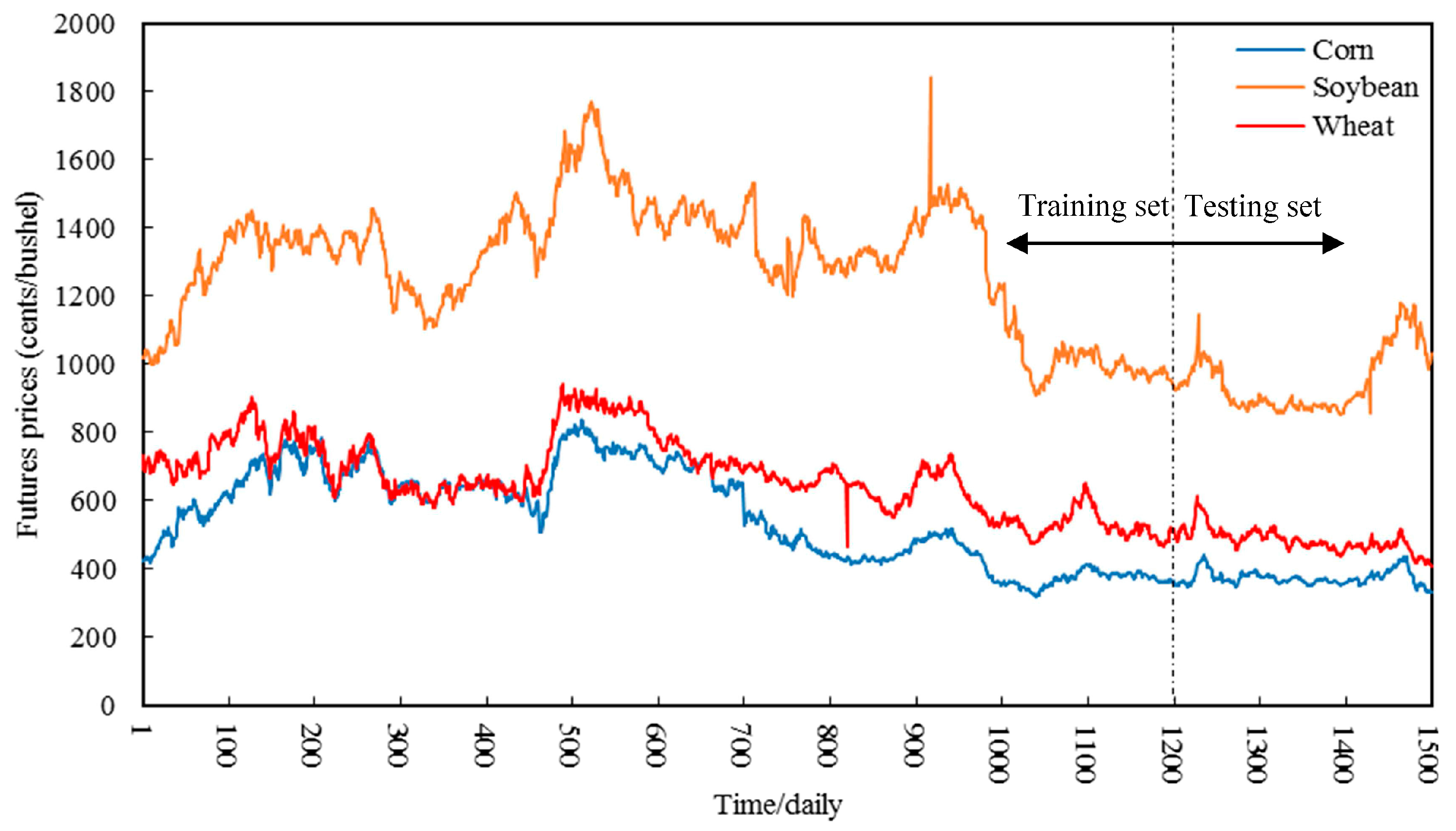
Based on the above detailed description and discussion, this section concentrates on the empirical results and analysis of the forecast day-ahead prices of the wheat, corn, and soybean futures, utilizing four hybrid predictive models, namely the WPT–PSO–BPNN model, the EMD–PSO–BPNN model, the ITD–PSO–BPNN model, and the VMD–PSO–BPNN model, respectively.

4.1. Case of Wheat Futures

In this paper, we focus on one-step-ahead forecasting models so that, with regard to a time series, a certain number of previous data are chosen as the input of the PSO–BPNN model to forecast the latter one, since the length of input may affect models’ forecasting accuracy in some degree. According to comparative analysis of several prediction results with different input length, the optimal length of the PSO–BPNN’s input series turns out to be eight; that is, with regard to a time series $\left\{X_t,t=1,2,\dots ,n\right\}$, this study uses $\left\{X_1,X_2,X_3,X_4,X_5,X_6,X_7,X_8\right\}$ to forecast $X_9$; and so on, $X_{i+8}$ can be forecasted by $\left\{X_i,X_{i+1},X_{i+2},X_{i+3},X_{i+4},X_{i+5},X_{i+6},X_{i+7}\right\}$. Meanwhile, some main parameters of the PSO algorithm and BPNN are set as shown in

Table 2. Main parameters ¹ settings of particule swarm optimization (PSO) and BPNN.

Algorithm	Parameters
PSO	c1	2	vmax	0.5
	c2	2	minerr	0.001
	wmax	0.9	wmin	0.3
	itmax	100	N	40
BPNN	innum	8	hiddennum	2
	outnum	1	epochs	100
	goal	0.00001	lr	0.1

¹ The c1 and c2 are two acceleration coefficients; and vmax means maximum velocity of particles while minerr is the minimum error; and wmax and wmin represent the maximum and minimum of the inertia weight; N and itmax denote length of particles and max iterations, respectively; and innum, hiddennum and outnum are the number of nodes in the input layer, the hidden layer and the output layer, respectively.

. It should be noted that the parameters listed in Table 2 are determined through a number of empirical experiments.

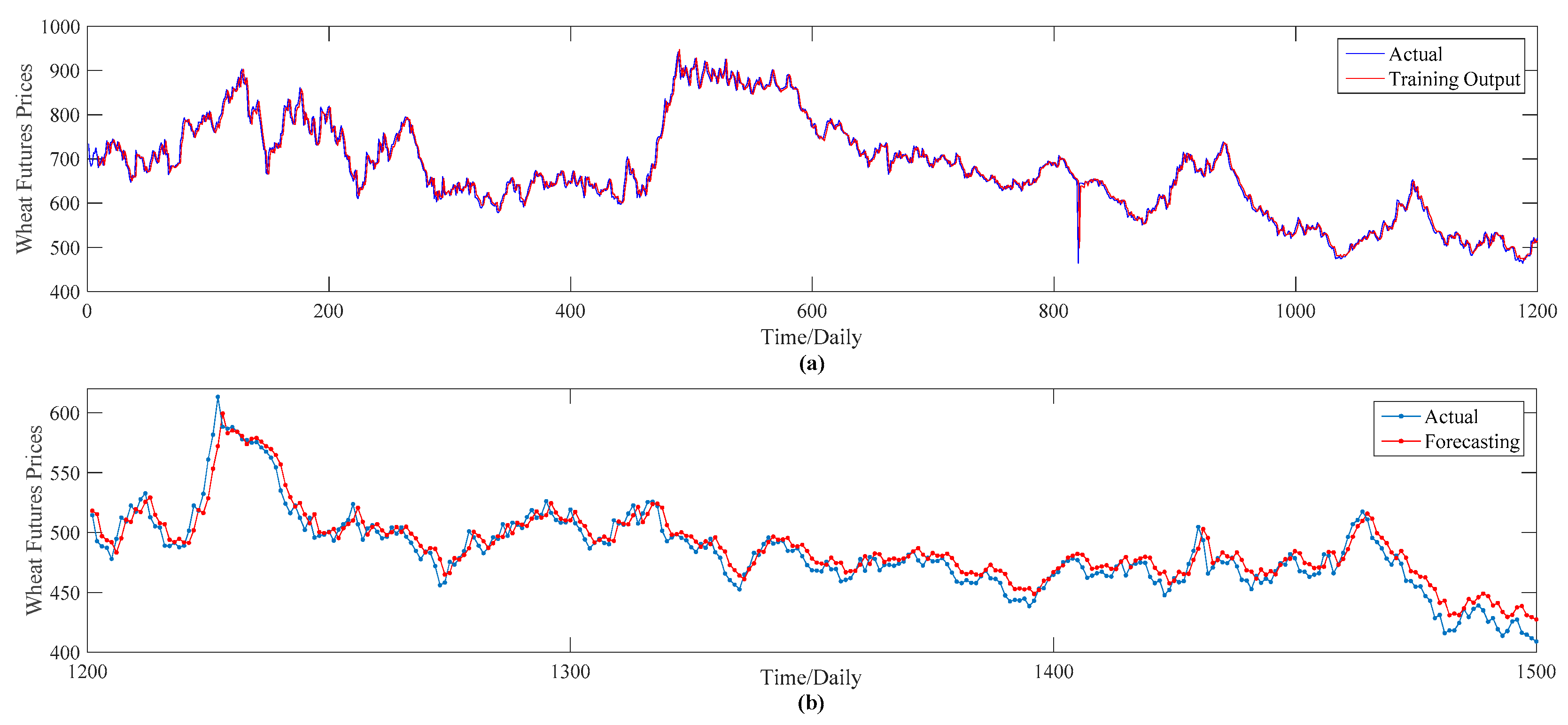
Based on the input length and the main parameter settings of the forecasting model, we use these to conduct our empirical study; this model’s training performance and forecasting performance are shown in Figure 6a,b, respectively. From this figure, it is obvious that not only the training output values but the predictions are also extremely close to the actual values, meaning that the PSO–BPNN model performs well in forecasting wheat futures prices. In the next discussion of this section, we regard the PSO–BPNN model as the benchmark model to compare its forecasting accuracy with the other four hybrid models proposed in this study. In order to compare the effectiveness of the EMD, WPT, ITD and VMD approaches respectively, we maintain the same parameter settings of this PSO–BPNN model with the four hybrid models throughout the whole paper.

4.1.1. Decomposition Results

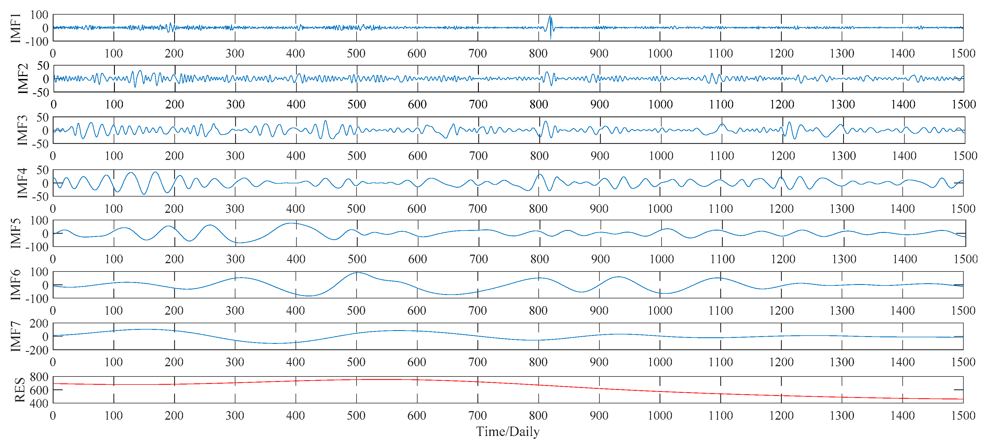
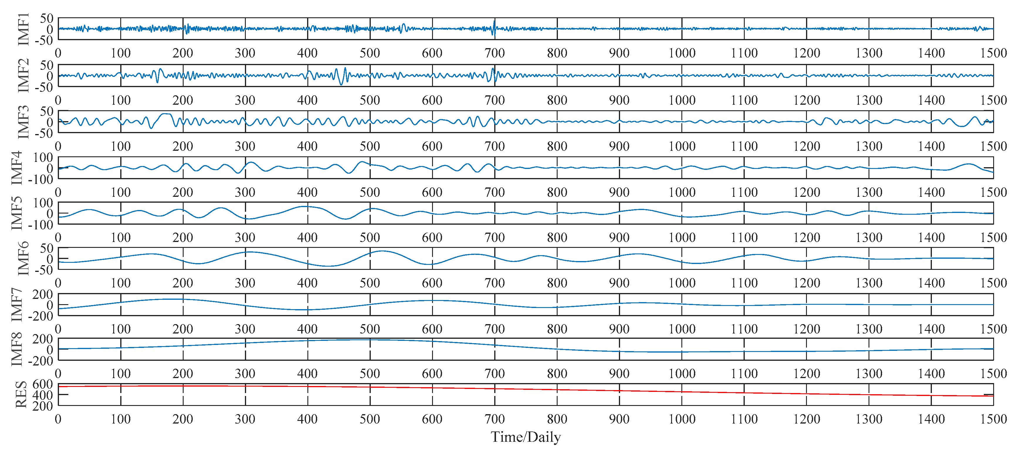
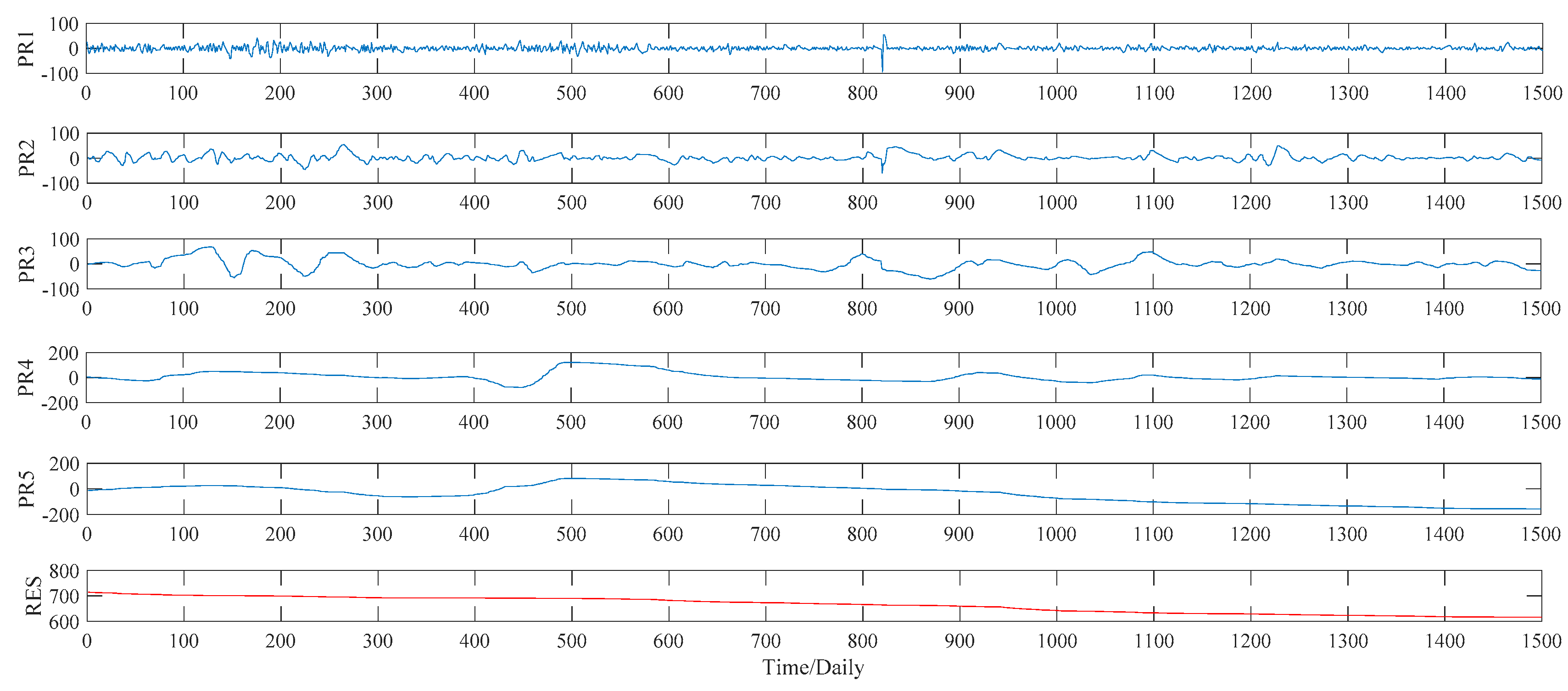
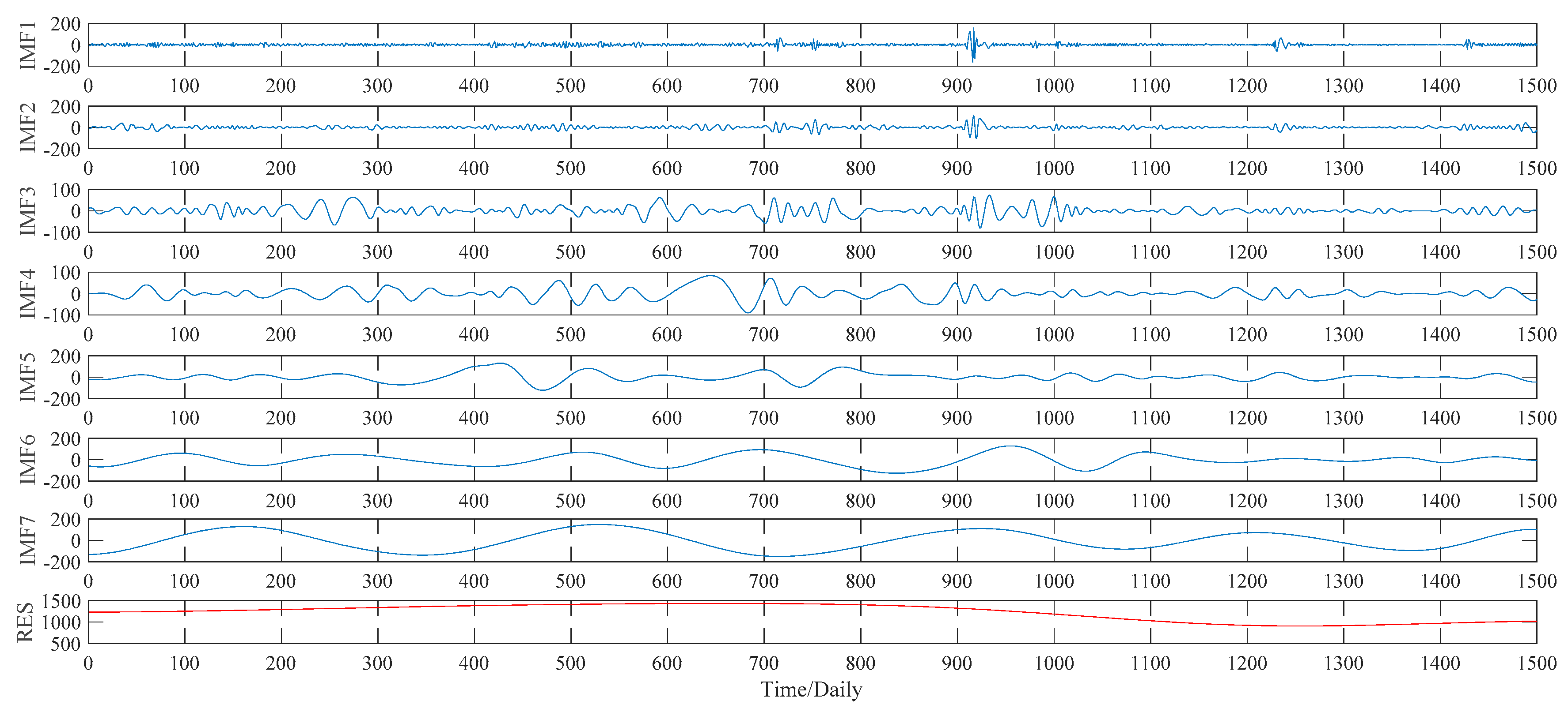
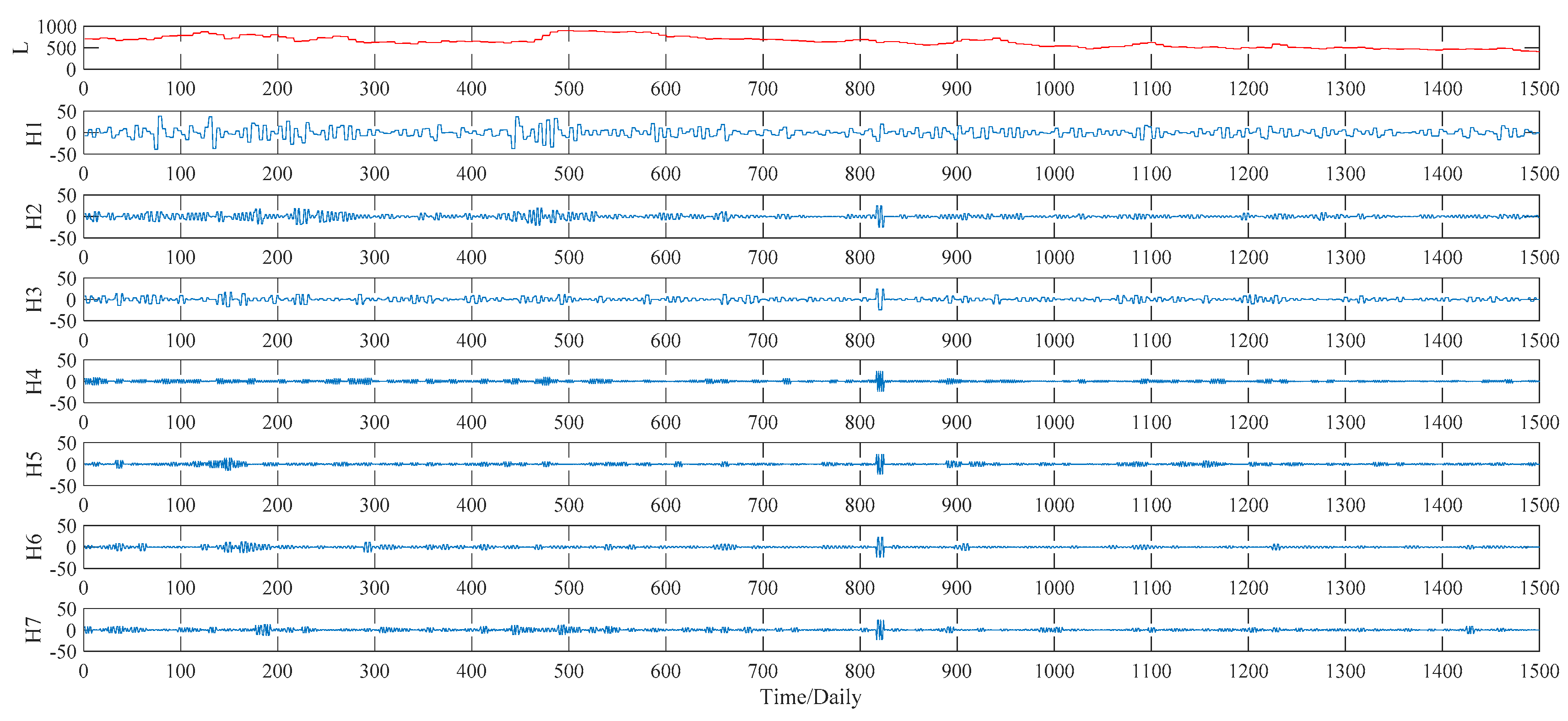
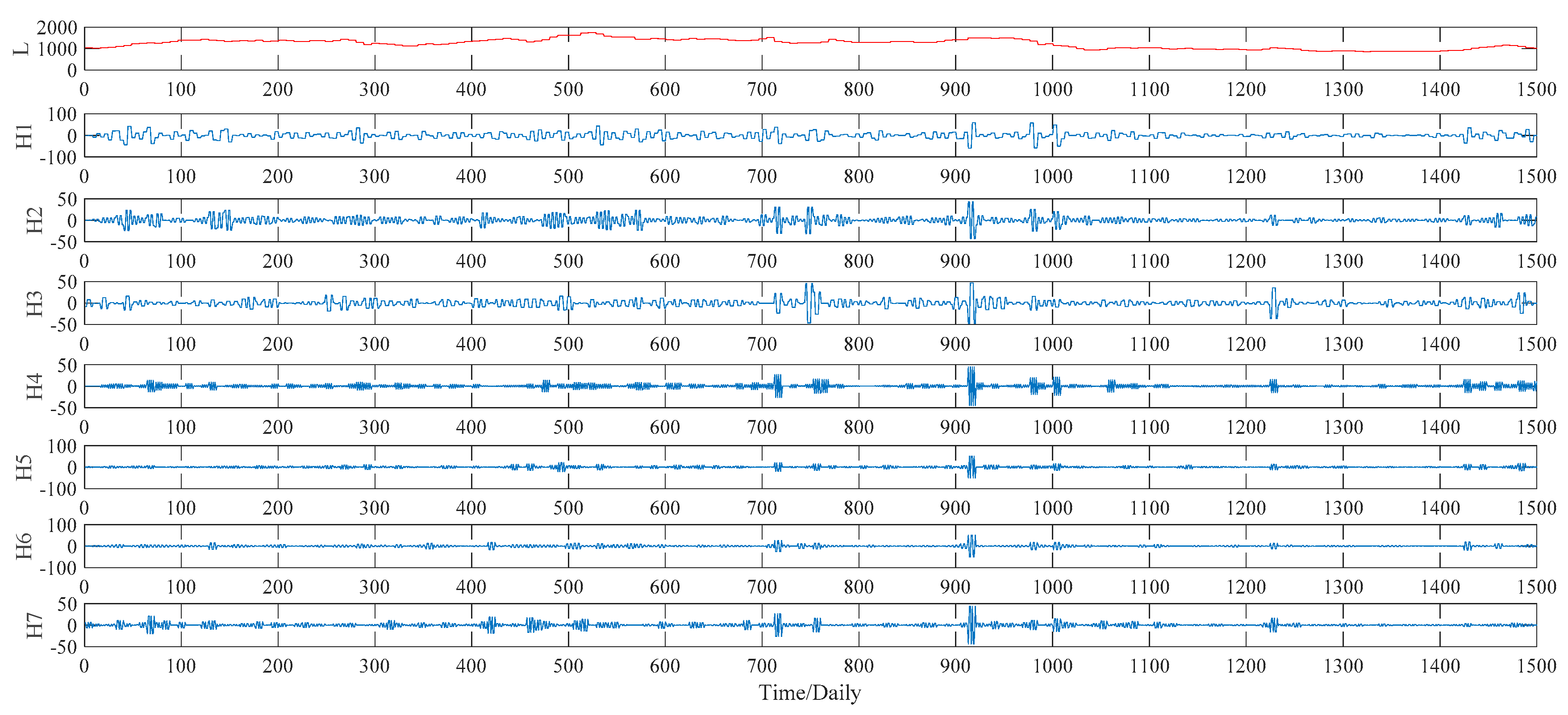
This subsection illustrates the decomposition results of wheat futures prices using EMD, WPT, ITD and VMD approaches, respectively. More specifically, according to the EMD method, the price data series of wheat futures is decomposed into seven IMFs, defined as IMF1, IMF2, …, IMF7, and a residual sub-series, named RES, which are shown in Figure 7. As to the WPT method, two typical decomposition levels, namely two levels and three levels, are taken into consideration in our study, for the sake of finding out the better decomposition level that will improve the PSO–BPNN’s forecasting accuracy more. 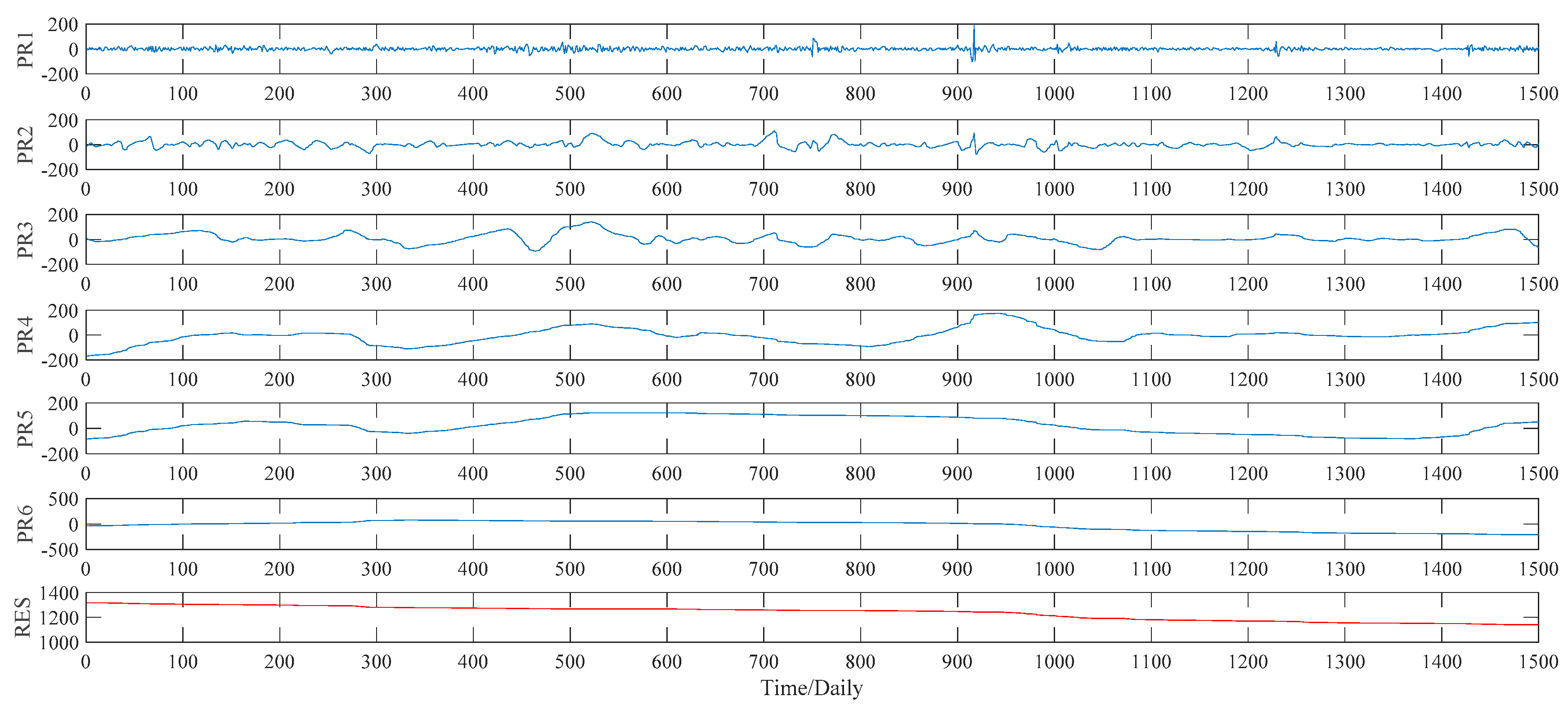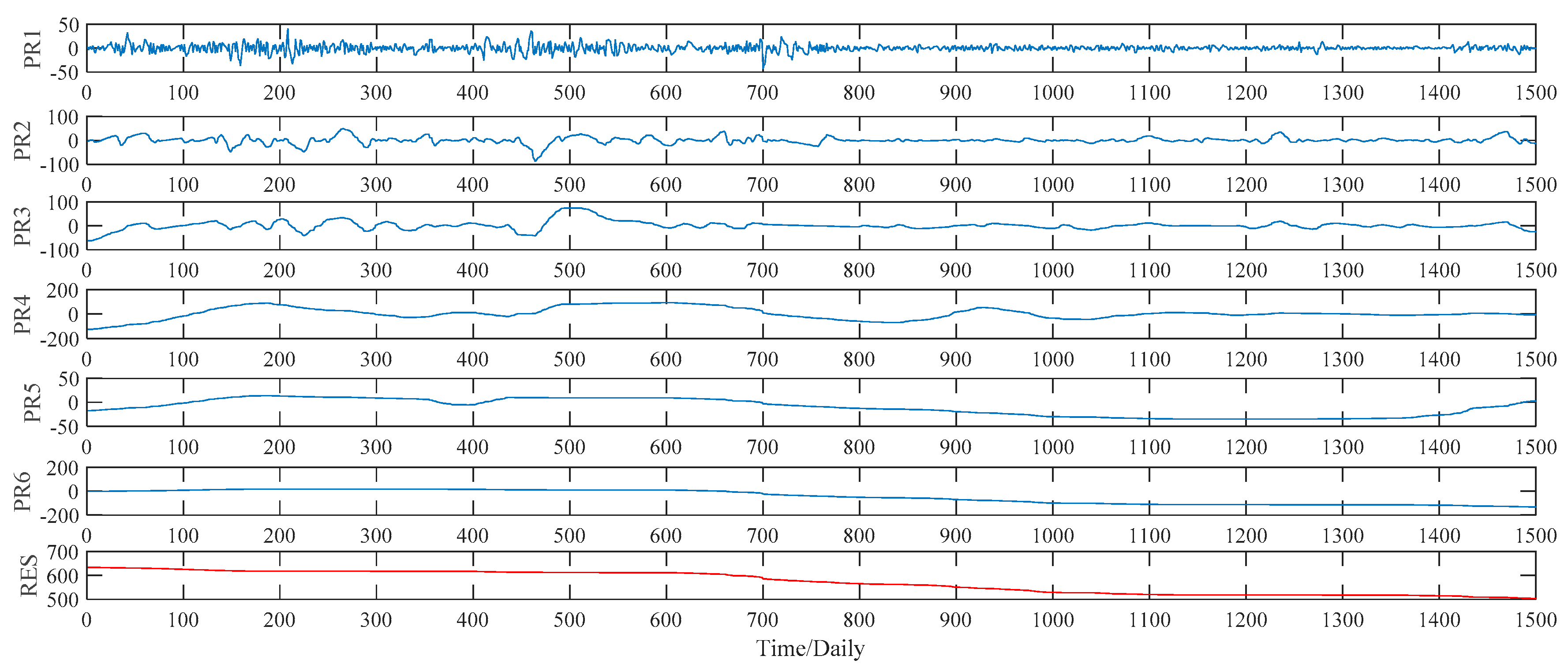Finally, the more suitable level turns out to be three, and the three-level decomposition results, including an approximation component L and seven detail components defined as H1, H2, …, H7, of the WPT technique is given in Figure 8. As to the ITD method, the upper limit on the number of decomposition, namely ten, is set manually in our study. Under such a preset, the ITD method automatically divides the sample data into five PRs, and a RES as well. 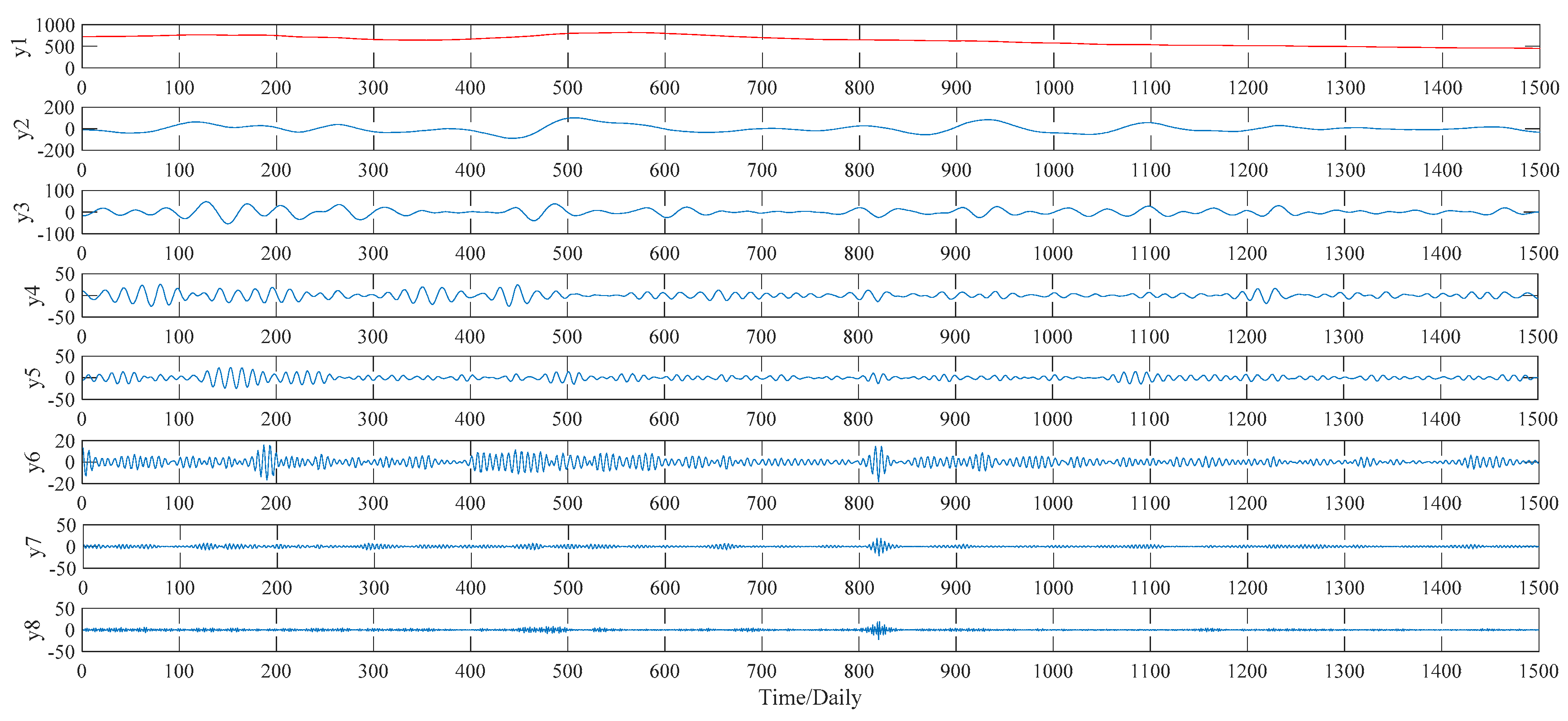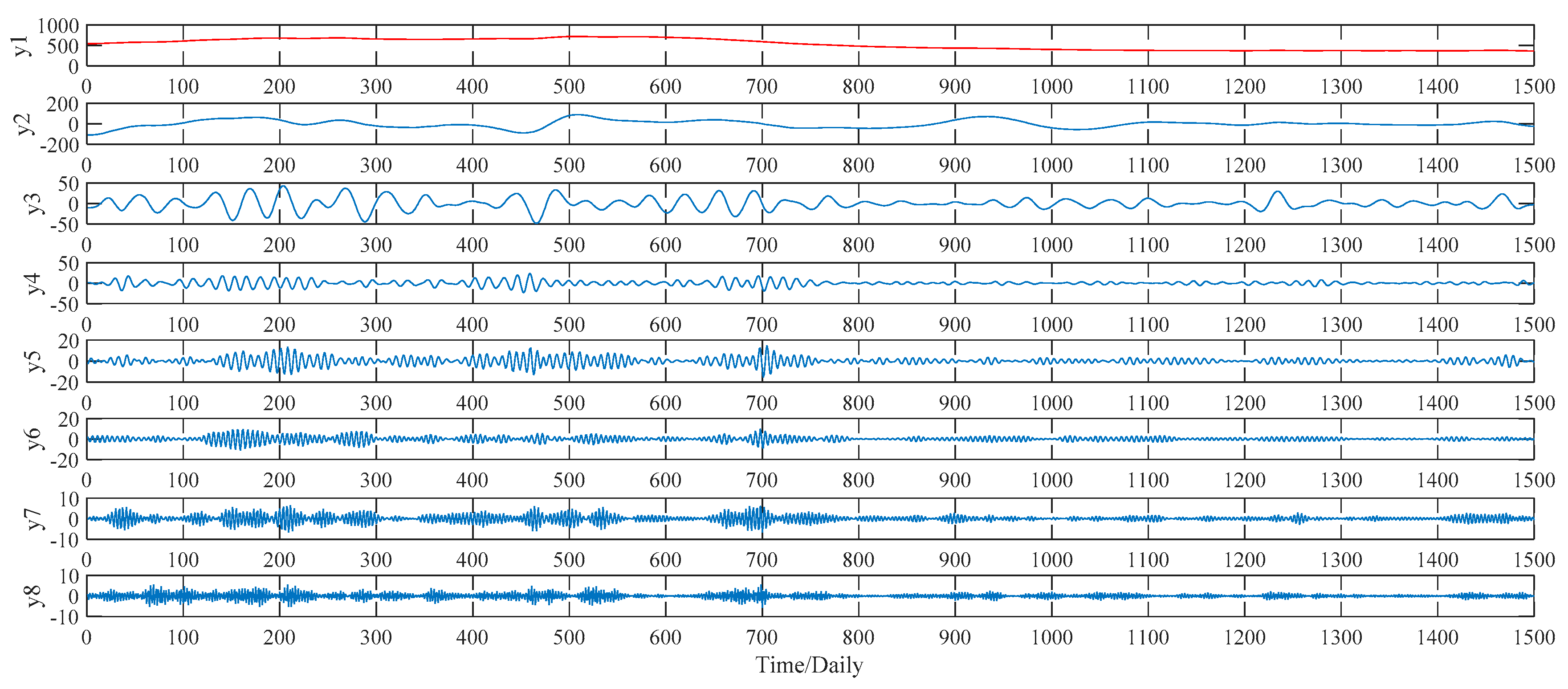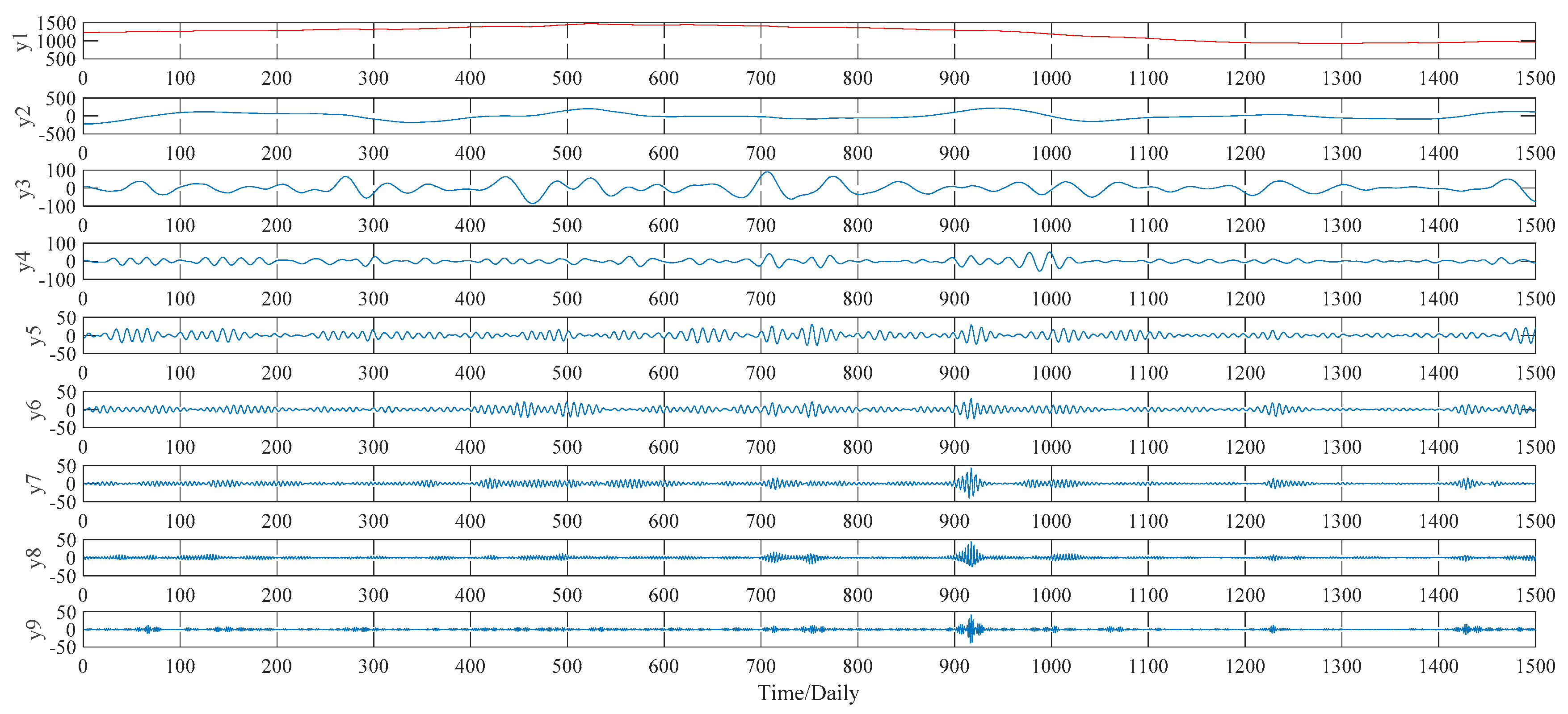See Figure 9 for decomposition results in detail. As to the VMD method, this study compares the decomposition effect of different number of modes, namely from six modes to nine modes. Given the hybrid models’ forecasting accuracy, eight modes, namely y1, y2, …, y8,, are determined eventually, as shown in Figure 10.

4.1.2. Comparison and Analysis

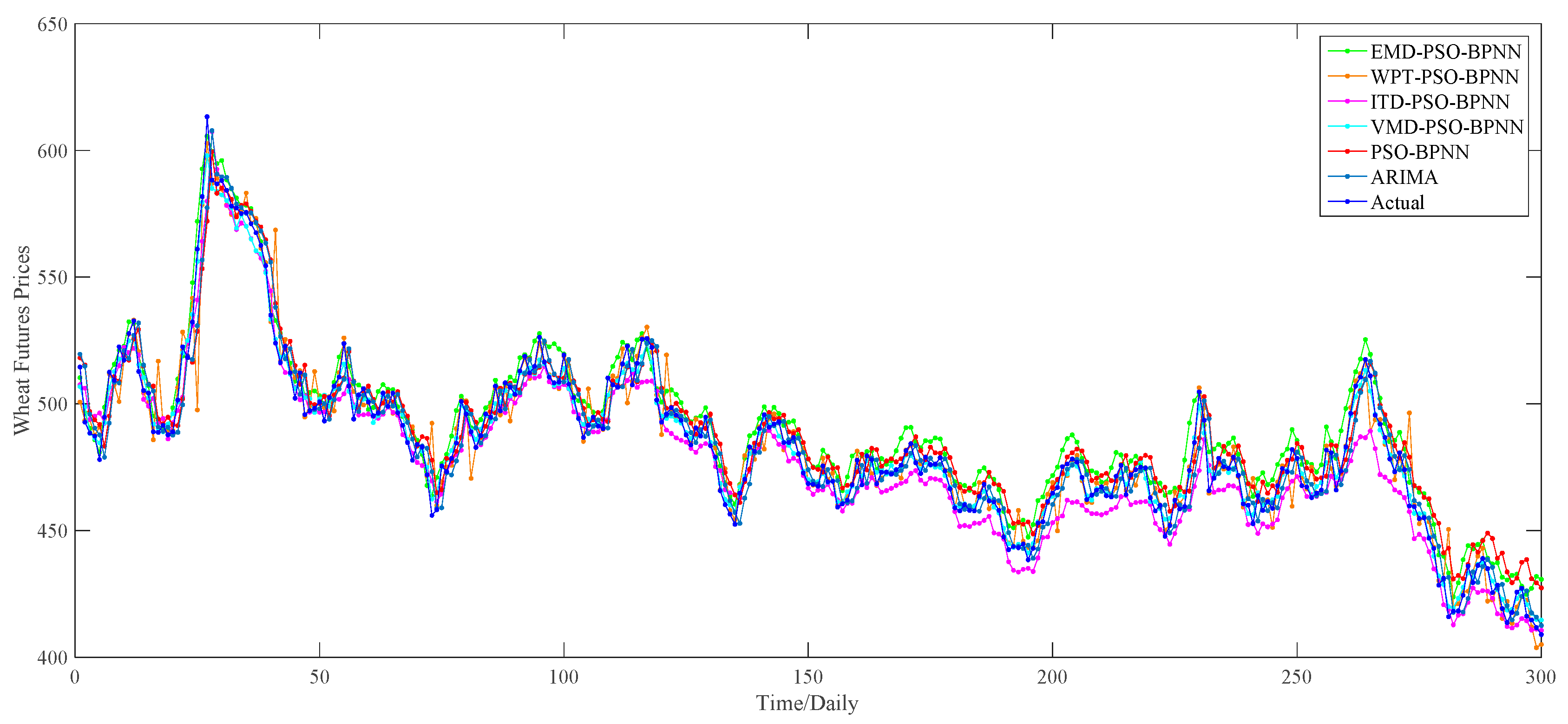
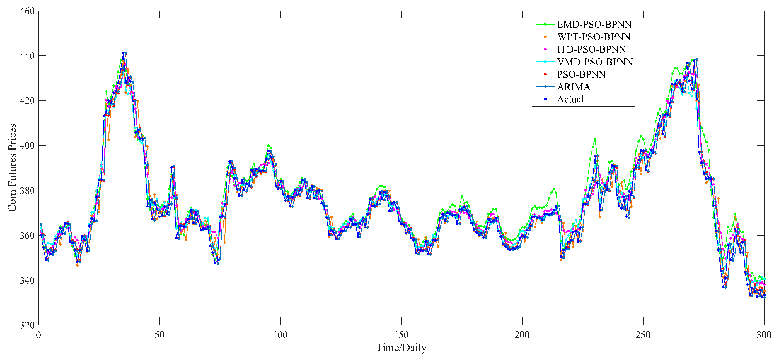
Based on the decomposition results of these four decomposition methods shown in Section 4.1.1, we apply the PSO–BPNN model to implement the forecasting part. As for the decomposition results of each decomposition algorithm, the PSO–BPNN model is utilized to predict the last 20 percent of data, namely 300 forecasting values totally, of each sub-series. Then, 300 predictions of each sub-series are summed up in order to obtain the ultimate 300 forecasting values of the wheat futures prices. For a better comparison of the effectiveness of four hybrid models combined with four different decomposition techniques, we select the PSO–BPNN model without decomposition methods as a benchmark model, aiming to testify the effectiveness of decomposition techniques. Furthermore, the ARIMA model is treated as a comparative model in order to compare the superiority in predictive capability between the ANN-based models and the traditional statistic models. 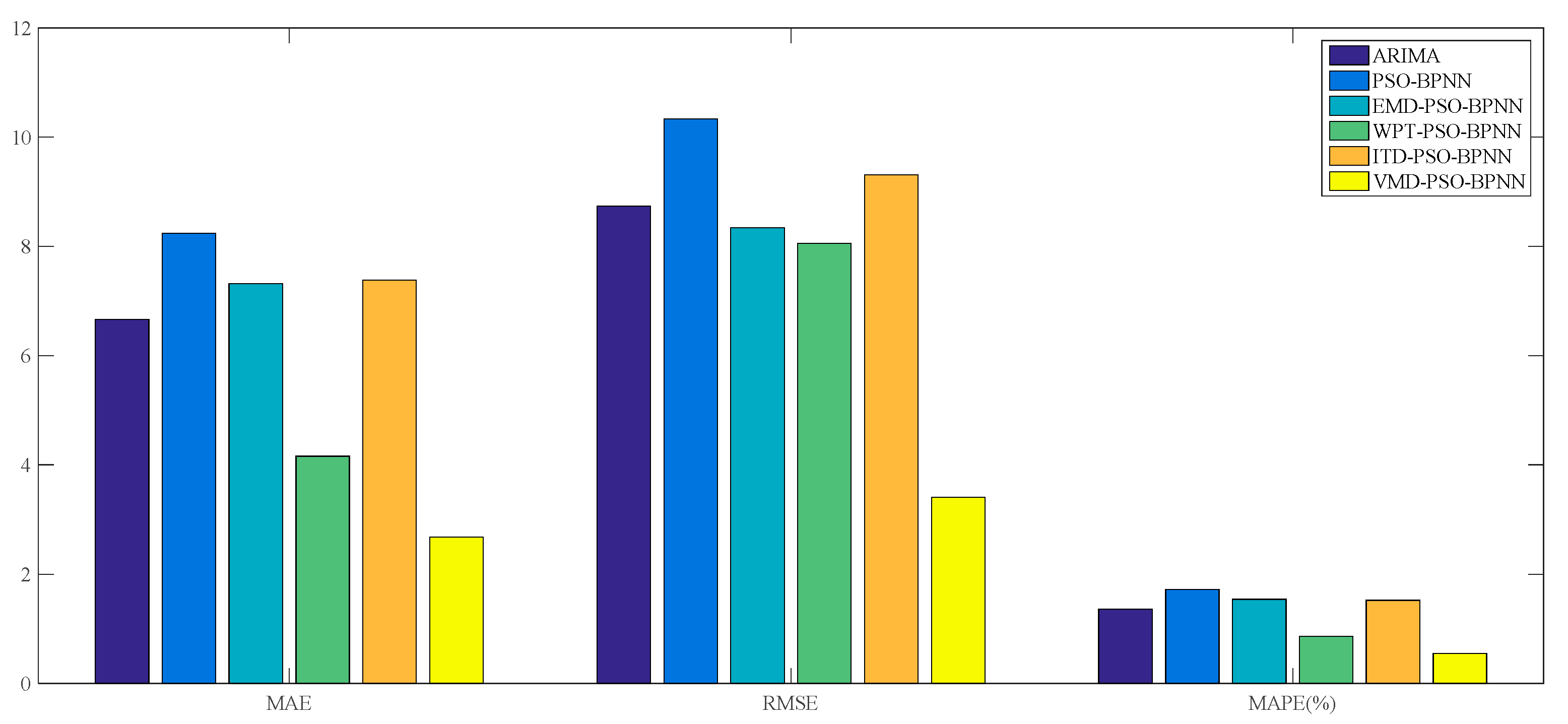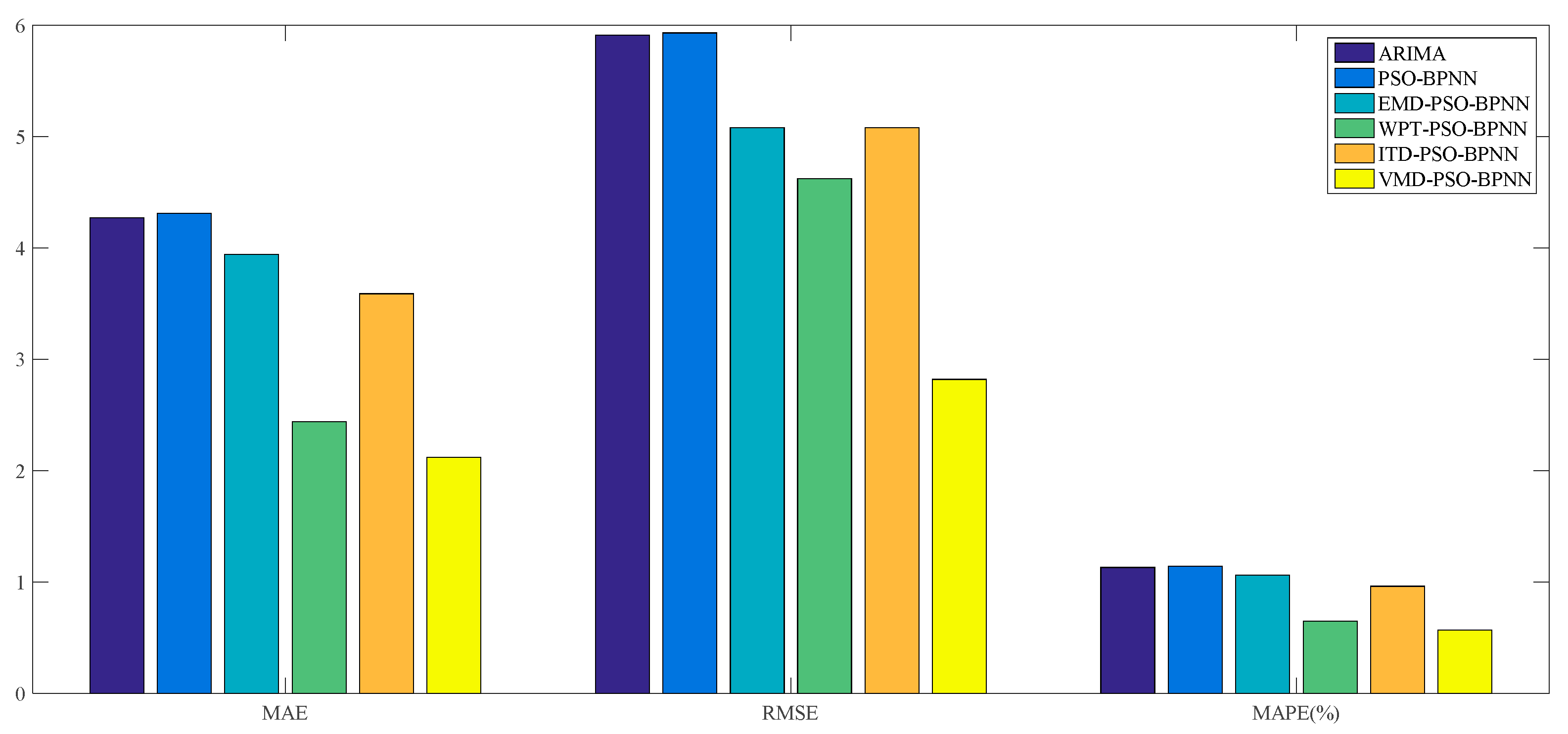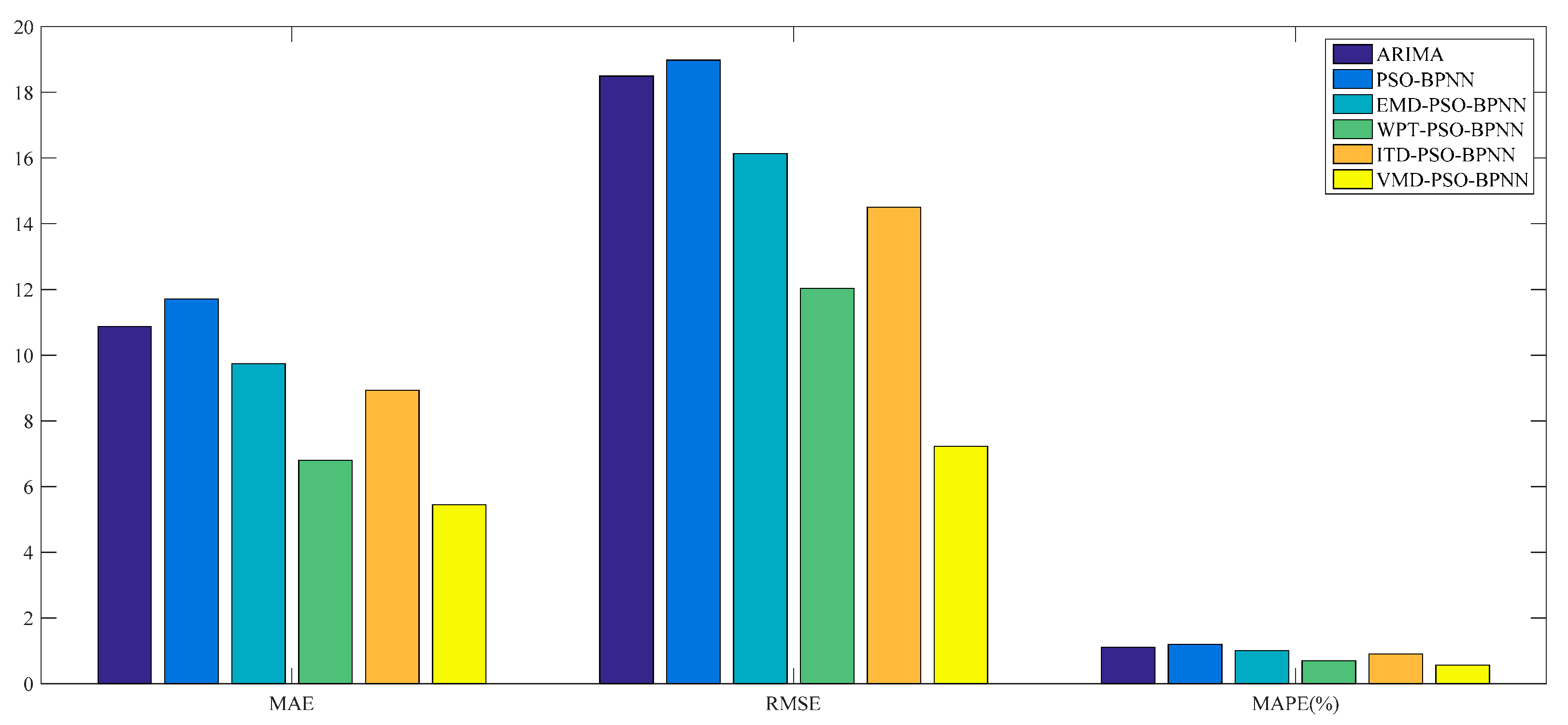The comparison of one-day-ahead forecasting results among all these models is provided in Figure 11. And the forecasting performance is evaluated through three criteria, namely the MAE, RMSE and MAPE, which are given in

Table 3. Forecasting performance evaluation of wheat.

Models	Criteria
	MAE	RMSE	MAPE (%)
PSO–BPNN	8.24	10.33	1.72
EMD–PSO–BPNN	7.32	8.34	1.54
WPT–PSO–BPNN	4.16	8.06	0.86
ITD–PSO–BPNN	7.38	9.31	1.52
VMD–PSO–BPNN	2.68 *	3.41 *	0.55 *
ARIMA	6.66	8.74	1.36

* The smallest value of each column is marked in boldface and with an asterisk. MAE: mean absolute error; RMSE: root mean square error; MAPE: mean absolute percentage error.

and Figure 12.

According to the Figure 11, there exists a preliminary judgment that the forecasting accuracy of the VMD–PSO–BPNN model is higher than any other model proposed in this study, since, during the whole forecasting period, the predictions of this model and actual values always keep a relatively high degree of coincidence compared with others, especially during the second half of the forecasting period.

Furthermore, it can be proved from Table 3 that, among all these forecasting models mentioned above, the VMD–PSO–BPNN model performs much better than any other model; namely the EMD–PSO–BPNN model, WPT–PSO–BPNN model, ITD–PSO–BPNN model, PSO–BPNN model and ARIMA model, in terms of the values of MAE, RMSE and MAPE, which respectively are 2.68, 3.41 and 0.55% for the VMD–PSO–BPNN model.

For the comparison among ANN-based models, more specifically, on the one hand, the EMD–PSO–BPNN model, WPT–PSO–BPNN model, ITD–PSO–BPNN model and VMD–PSO–BPNN model have a more satisfactory performance than the PSO–BPNN model in terms of these three evaluation criteria, which means that the decomposition methods mentioned in this study can further make the PSO–BPNN model improve its forecasting accuracy of wheat futures; on the other hand, the VMD–PSO–BPNN model shows considerable superiority compared with other hybrid models combined with EMD, WPT and ITD methods respectively, signifying that the VMD method is proven to be more effective to conduct data pretreatment in contrast to the other three decomposition approaches. From a pure data perspective, the values of MAE, RMSE and MAPE of the VMD–PSO–BPNN model have all been reduced by about 68% compared with the PSO–BPNN model and approximately 63% compared with the ITD–PSO–BPNN model, and have decreased by 63.39%, 59.11% and 62.34% respectively compared with the EMD–PSO–BPNN model, and 35.58%, 57.09% and 36.05% respectively compared with the WPT–PSO–BPNN model.

For the comparison between ANN-based models and the ARIMA model, in terms of the MAPE, the value of ARIMA model is a little smaller than the PSO–BPNN model, EMD–PSO–BPNN model and ITD–PSO–BPNN model, while its value is obviously much larger than the WPT–PSO–BPNN model and VMD–PSO–BPNN model.

On the whole, it can be concluded that the WPT–PSO–BPNN model and VMD–PSO–BPNN model, especially the latter one, are more suitable to be used in forecasting the wheat futures prices because they raise the forecasting precision, namely the MAPE, by an order of magnitude, in contrast with the ARIMA model, PSO–BPNN model, EMD–PSO–BPNN model and ITD–PSO–BPNN model. The reasons why the forecasting accuracy of VMD-based hybrid model is superior to other hybrid models lie in the following two causes: (1) the VMD based model searches for a number of modes and their respective center frequencies, such that the band-limited modes reproduce the input signal exactly or in least-squares sense, thus VMD has the ability to separate components of similar frequencies compared with other decomposition methods; (2) VMD is more robust to noisy data such as wind speed, PM_2.5 concentration and agricultural commodity future price. Indeed, since each mode is updated by Wiener filtering in Fourier domain during the optimization process, the updated mode is less affected by noisy disturbances, and therefore the VMD can be more efficiently for capturing signal’s short and long variations than other decomposition methods [52].

4.2. Case of Corn Futures

Although wheat, corn and soybean prices are strongly correlated [15], it is still necessary to conduct certain research on different food grain futures in order to verify the applicability and validity of the hybrid models with decomposition methods developed in our study on the aspect of prices forecasting. Thus, this subsection presents the empirical study of forecasting the corn futures prices on the basis of these hybrid models, and the empirical study of soybean futures prices is in the next subsection. Similarly, decomposition results of corn futures prices, based on the EMD, WPT, ITD and VMD techniques respectively, are shown from Figure 13, Figure 14, Figure 15 and Figure 16, and the comparison between the one-day-ahead predictions and actual values are given in Figure 17, while the forecasting performance evaluation results are displayed in

Table 4. Forecasting performance evaluation of corn.

Models	Criteria
	MAE	RMSE	MAPE (%)
PSO-BPNN	4.31	5.93	1.14
EMD-PSO-BPNN	3.94	5.08	1.06
WPT-PSO-BPNN	2.44	4.62	0.65
ITD-PSO-BPNN	3.59	5.08	0.96
VMD-PSO-BPNN	2.12 *	2.82 *	0.57 *
ARIMA	4.27	5.91	1.13

* The smallest value of each column is marked in boldface and with an asterisk.

and Figure 18, respectively.

Likewise, the empirical results show that the VMD–PSO–BPNN model still outperforms the EMD–PSO–BPNN model, WPT–PSO–BPNN model, ITD–PSO–BPNN model, PSO–BPNN model and ARIMA model, with respect to the forecasting performance evaluation criteria, on the basis of Table 4 and Figure 18. But the disparity of forecasting precision between the VMD–PSO–BPNN model and other models is reduced. More specifically, for the comparison among all ANN-based models, similar conclusions with the study case of wheat can be obtained; that is, in respect of the MAE, RMSE and MAPE, the VMD–PSO–BPNN model and WPT–PSO–BPNN model perform much better than the other three models, while the ITD–PSO–BPNN model and EMD–PSO–BPNN model only improve a little compared with the PSO–BPNN model. For the comparison between the ANN-based models and the ARIMA model, all hybrid models with decomposition approaches outperform the ARIMA model, while the PSO-BPNN model (1.14%) almost shares the same forecasting accuracy with the ARIMA model (1.13%) in terms of the evaluation criterion, MAPE.

Moreover, it is worthy of note that there are three hybrid models, combined with the WPT, ITD and VMD respectively, whose forecasting accuracy is improved by one order of magnitude to 0.65%, 0.96% and 0.57%, respectively.

4.3. Case of Soybean Futures

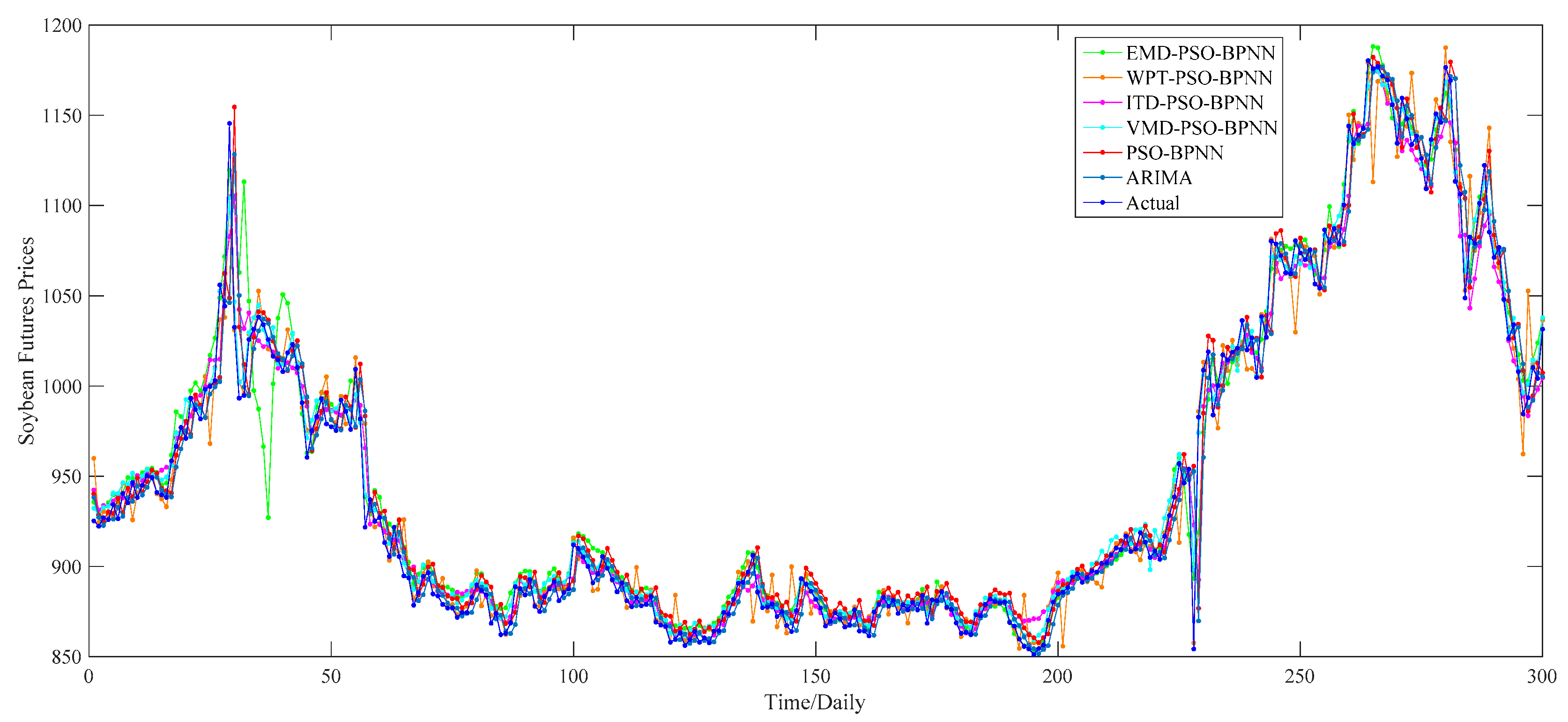
Similarly, the EMD, WPT, ITD and VMD methods are applied to decompose the soybean futures prices in this subsection, whose decomposition results are given from Figure 19, Figure 20, Figure 21 and Figure 22, respectively. Based on the decomposition results, we use the four proposed “decomposition and ensemble” hybrid models to forecast the soybean futures prices during the period from 10 August 2010 to 29 July 2016, totally 300 values, regarding the PSO–BPNN model as the benchmark model and ARIMA model as the comparative model. The comparison of the one-day-ahead forecasting results is drawn as shown in Figure 23 and Figure 24 and

Table 5. Forecasting performance evaluation of soybean.

Models	Criteria
	MAE	RMSE	MAPE (%)
PSO-BPNN	11.71	18.98	1.20
EMD-PSO-BPNN	9.74	16.13	1.01
WPT-PSO-BPNN	6.80	12.03	0.70
ITD-PSO-BPNN	8.93	14.50	0.91
VMD-PSO-BPNN	5.45 *	7.22 *	0.57 *
ARIMA	10.87	18.49	1.11

* The smallest value of each column is marked in boldface and with an asterisk.

, respectively.

According to these figures and table, we can reach conclusions similar to the empirical research on the wheat and corn; i.e., that the VMD–PSO–BPNN model is still the best model to forecast the soybean futures prices among all models proposed in this paper. Based on the value of MAPE, the order of these six models, from big to small, is the PSO–BPNN model (1.20%), ARIMA model (1.11%), EMD–PSO–BPNN model (1.01%), ITD–PSO–BPNN model (0.91%), WPT–PSO–BPNN model (0.70%) and VMD–PSO–BPNN model (0.57%), which shows that hybrid models with decomposition methods, especially the VMD method, have obvious advantages in forecasting the soybean futures prices in contrast with the PSO–BPNN model and ARIMA model.

5. Conclusions

As the world’s leading and most diverse derivatives marketplace, CME Group’s wheat, corn and soybean futures prices are not only important reference prices of agricultural production and processing but also the authority of prices in the international trade of agricultural products, which can reflect the change trend of the corresponding agricultural products’ spot prices in advance to some extent. Thus, forecasting their prices is expected to be an effective method for controlling market risks and making appropriate and sustainable food grain policy for the government. However, current research pays little attention to forecasting food grain futures prices and does not take their nonlinear and nonstationary characteristics into account while making predictions. Based on the above consideration, we propose four hybrid models which combine the PSO–BPNN model with the EMD, WPT, ITD and VMD methods respectively, to forecast wheat, corn and soybean futures prices, which can enrich empirical research on agricultural commodity futures prices forecasting, to some extent.

According to our experimental results, three main conclusions are drawn as follows: (1) it has been proved that the VMD–PSO–BPNN model outperforms the EMD–PSO–BPNN model, WPT–PSO–BPNN model, ITD–PSO–BPNN model, PSO–BPNN model and ARIMA model in all study cases, in terms of three forecasting performance evaluation criteria, namely the MAE, RMSE and MAPE, which suggests that the proposed VMD–PSO–BPNN model has a high common adaptability and serviceability in forecasting the wheat, corn and soybean futures prices; (2) in all study cases, the forecasting performance of all four hybrid models with decomposition methods are superior to the performance of the PSO–BPNN model, which demonstrates that the EMD, WPT, ITD and VMD methods play an extremely significant role in improving the PSO–BPNN model’s forecasting performance of these futures prices; (3) after comparing the results of different “decomposition and ensemble” hybrid models, we find out that the prediction ability of VMD–PSO–BPNN model and WPT–PSO–BPNN model is much better than the ability of EMD–PSO–BPNN model and ITD–PSO–BPNN model, meaning that the VMD and WPT methods, especially the VMD method, are more suitable to be applied to analyzing the prices data of wheat, corn and soybean futures than other two approaches, namely the EMD and ITD.

Conclusively, based on the three evaluation criteria, four “decomposition and ensemble” hybrid models developed in this study perform better than the forecasting model without decomposition techniques, namely the PSO–BPNN model, with respect to the price forecasting of the wheat, corn and soybean futures, which provides a new promising research approach to forecasting prices of agricultural commodity futures.