Abstract
This is the first paper to present such a digital redesign method for the (conventional) OKID system and apply this novel technique for nonlinear system identification. First, the Observer/Kalman filter Identification (OKID) method is used to obtain the lower-order state-space model for a stochastic chaos system. Then, a digital redesign approach with the high-gain property is applied to improve and replace the observer identified by OKID. Therefore, the proposed OKID combined with an observer-based digital redesign novel tracker not only suppresses the uncertainties and the nonlinear perturbations, but also improves more accurate observation parameters of OKID for complex Multi-Input Multi-Output systems. In this research, Chen’s stochastic chaotic system is used as an illustrative example to demonstrate the effectiveness and excellence of the proposed methodology.
1. Introduction
In the past decade, many system identification techniques have been developed and applied to identify a state-space model for modal parameter identification of large flexible space structures [1]. Theoretically, for a nonlinear system with precise differential equations, a higher-order linear model always gives a better approximation than a lower-order one. Therefore, how to pre-specify an appropriate lower-order system and its initial parameters to identify a nonlinear system scheme is quite important and technically challenging.
Recalling a well-known early approach for system identification based on the concept of minimum realization, Kalman proposed a state-space model of the lowest possible dimension among all realizable systems and constructed effective linear state-variable models from input-output data [2]. After that, the Observer/Kalman filter Identification (OKID) technique is an extension of an eigensystem realization algorithm (ERA) that permits efficient identification of large flexible structures [3]. Based on the concepts of stochastic estimation and techniques of deterministic Markov parameter identification, OKID directly generates a local linear state-space model for the underlying nonlinear system. The OKID method also shows a valuable tool for model linearization, which has proven to be an effective lower-order identification in spacecraft identification problems [4,5] and a stochastic chaotic hybrid system [6].
The digital redesign method is applied to discretize a continuous-time control system, which has been widely used in industries and proven successful for several control strategies [7]. The desirable observer design approach of the redesign system is to use the minimum error energy concept to minimize the performance index and obtain an optimal observer so that the estimated error compared with the original dynamics signal can be minimized and quickly convergent [8].
This is the first paper to present such a digital redesign method for the (conventional) OKID system. The developed methodology was realized on the nonlinear system and showed the proposed method is about 10 times more accurate than the only OKID algorithm. In our experiment, the OKID algorithm is proposed to provide a lower-order identification system for Chen’s chaos system, and the digital redesign method is implemented to redesign the OKID system. By comparing the original signal with the estimated signal, the observer gain of the redesigned system could be obtained. The experimental result showed the combined method possesses a more accurate and robust system identification capability than the only OKID Algorithm. Our research shows a novel low-order observer-based digital redesign tracker for the equivalent chaotic system, and that it is theoretically possible to asymptotically track the stochastic chaos system with zero error.
2. OKID Formulation
2.1. Basic Observer Equation
The discrete-time, state-space model of the multivariable linear system can be represented in the following
where and are state, output, and control input vectors, respectively; and are system, input, and output matrices, respectively, and D is transmission matrix of input function .
By adding and subtracting an observer term [5] to the right-hand side of the function in Equation (2), yield the observer equation
where is considered as an observer state vector,
and is an arbitrary matrix that can be used to make the matrix as stable as desired. Therefore, the Markov parameters (, ) of the system in Equation (3) will be referred to as the observer Markov parameters. The mathematical development here can be interpreted as the point of view of [4] as attempting to place all the eigenvalues of at the origin.
Consider the case where is asymptotically stable so that for some sufficiently large , for all time steps .
Substituting in Equation (2) with Equation (4), results in
The set of Equation (5) for a sequence of can be written as
where is a unit matrix, is a constant,
and
Since will be approximated to zero, thus Equation (6) will be simplified to
From Equation (9), the least-squares solution is obtained
where is the pseudo-inverse of the matrix .
The matrices and are subsets of y and , respectively, produced by deleting the first q columns. For nonzero unknown initial conditions, Equation (9) must be used in order to eliminate the effect of initial conditions because the initial conditions become negligible when they are multiplied by . In other words, the initial conditions have negligible influence on the measured data after q time steps. When there are both system and measurement noises present, the elimination of initial condition dependence makes the system response become stationary, a fact which is used later to obtain the steady-state Kalman filter gain.
2.2. Computation of Markov Parameters
The observer Markov parameters include the system Markov parameters and the observer gain Markov parameters. The system Markov parameters are used to compute the system matrices , whereas the observer gain Markov parameters are used to determine the observer gain
2.2.1. System Markov Parameters
To recover the system Markov parameters in from the observer Markov parameters in , partition as
By derivation, the general relationship between the actual system Markov parameters and the observer Markov parameters is
2.2.2. Observer Gain Markov Parameters
To identify the observer gain first recover the sequence of parameters
By induction, the general relationship is
Form the Hankel matrix from the combined Markov parameters associated with the system and observer as
The ERA processes the factorization of the block data matrix in (19), started for via the singular value decomposition , where the columns of matrices and are orthonormal and is a rectangular matrix
where with monotonically non-increasing Simultaneous realizations of the system and observer by the ERA are given as
In practice, the primary purpose of introducing an OKID method is that the constructed observer satisfies the least-squares solution; if the data length is sufficiently long, and the order of the observer is sufficiently large, the truncation error is negligible. The low order of this model is forced to be [5].
Therefore, when the residual is a white sequence of the Kalman filter residual, the observer gain converges to the steady-state Kalman filter gain such that , where is the Kalman filter gain.
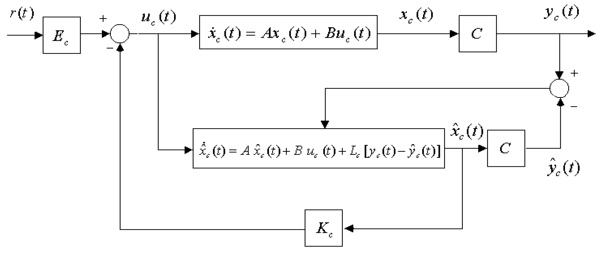
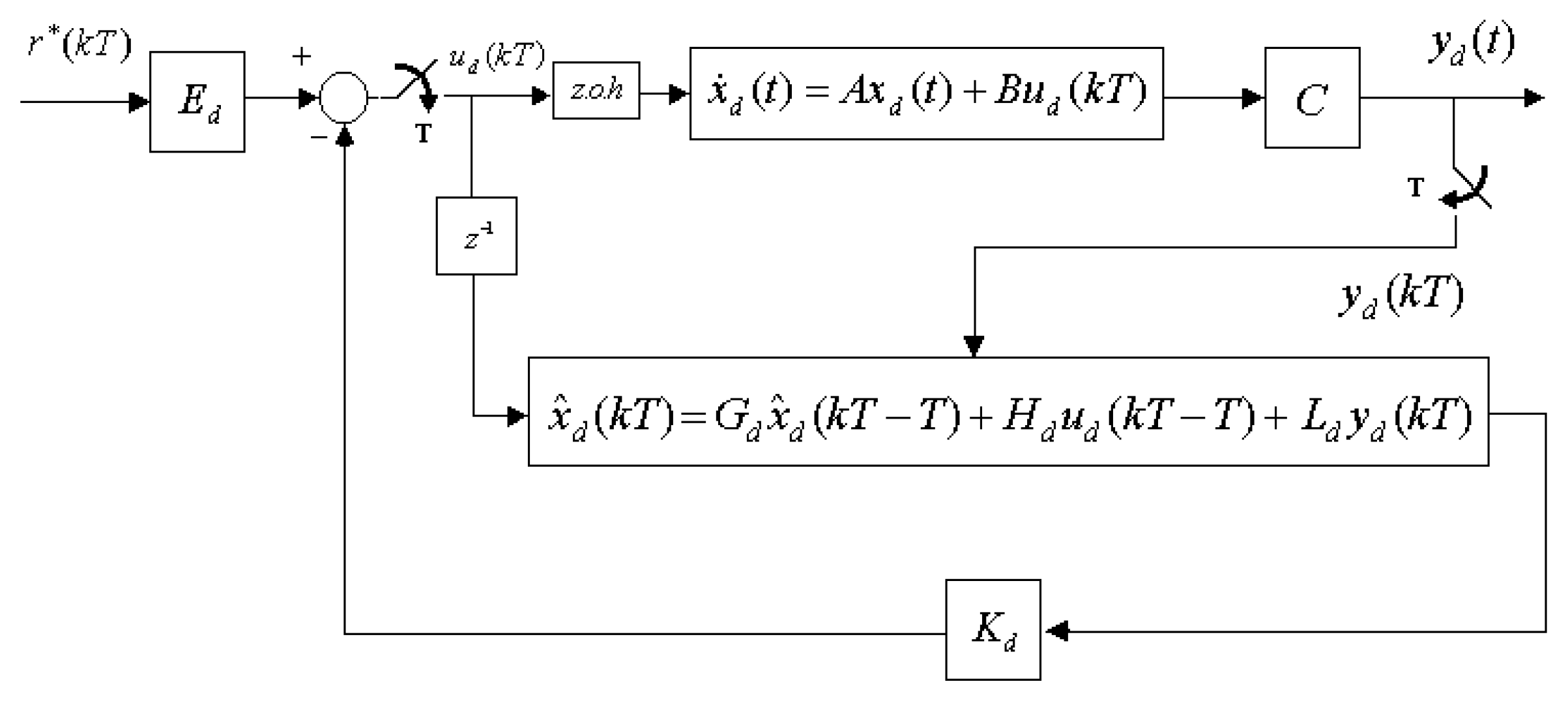
3. Digital Redesign of Full-Order Observer
Consider a linear observable continuous-time system described as
where , , and , , and are system matrices with appropriate dimensions. One method of estimating the unmeasured state is to construct a full-order model of the plant dynamics. The following derivation follows from [8]
To derive the dynamics of the observer, we consider feeding back the difference between the actual output and the estimated output, and correcting the model continuously with this error signal. The equation is as follows
Hence, the problem reduces designing an observer so that the error dynamics have their eigenvalues on the far left side of the complex s-plane, so the convergence to the original dynamics can be fast. Since the desirable observer design approach is to use the minimum error energy, an optimal design technique with a minimizing performance index is used.
In general, an optimal design of controllers for a given controllable and observable linear system is defined as shown in Equations (24) and (25), and the optimal state-feedback control law minimizes the performance index
with , , and are obtained as
where the optimal feedback gain is , with P being the positive definite and symmetric solution of the following Riccati equation [9]
In a closed loop, the optimal control linear system has the form of
Comparing Equations (32) and (28), we can see that
which has the structure as a state-feedback controller. This is the dual property of linear systems, where the observer gain can be determined as the dual of the feedback controller gain. Thus, the optimal observer gain can be found by designing the optimal control gain for the dual system, via and , so that ; or equivalently, , where P is the positive definite and symmetric solution of the Riccati equation
Now, since a continuous-time observer for the system presented in Figure 1 is defined in Equation (27), the next step is to find a digital observer for the system. First, define the discrete-time observer error as
Figure 1.
A continuous-time system with a full-order observer.
Therefore, the discrete-time error dynamics match the continuous-time error dynamics at each sampling instant , or, equivalently, assuming that the continuous-time observer is asymptotically stable, and the original state and the digital state match .
Using the duality once again, one can find the discrete-time error dynamics of Equation (28) as follows
where
Further defining , one can write and with substituting Equation (35) into Equation (36), it becomes
By substituting the following identities into Equation (37)
and solving the result for , one obtains the new digitally redesigned observer for (27)
or
where
The full-order observer-based sampled-data system is shown in Figure 2.
Figure 2.
Practically implemented full-order observer for the sampled-data linear system.
4. Effective Design Procedures for a Stochastic Chaotic System
The structure of the effective design procedure steps are shown as follows:
- Step 1.
- Perform the off-line system identification scheme to obtain both system and observer-gain Markov parameters of the OKID model.
- (i)
- Compute the observer Markov parameters. Choose a value of that determines the number of observer Markov parameters from the given set of input-output data, and then compute the least-squares solution of the Markov parameter matrix in Equation (10).
- (ii)
- Identify both system and observer-gain Markov parameters. Use the Markov parameters identified in (i) above, and Equations (14) and (18) to determine the combined system and observer-gain Markov parameters. Moreover, set up the Hankel matrix and as shown in Equation (19).
- (iii)
- Realize a state-space model of the system and the corresponding observer gain from the identified sequence of the system and observer-gain Markov parameters by using the ERA method to obtain the desired discrete system realization , and in Equations (21)–(23), where the non-causal term is assumed to be zero.
- Step 2.
- Set the full-order observer-based sampled-data system for the OKID combined with a digital redesign method.
- (i)
- Find the optimal observer gain . Select appropriate weighting matrices in Equation (34).
- (ii)
- By using the new digitally redesigned observer form, obtain the desired discrete system realization , and in Equation (38).
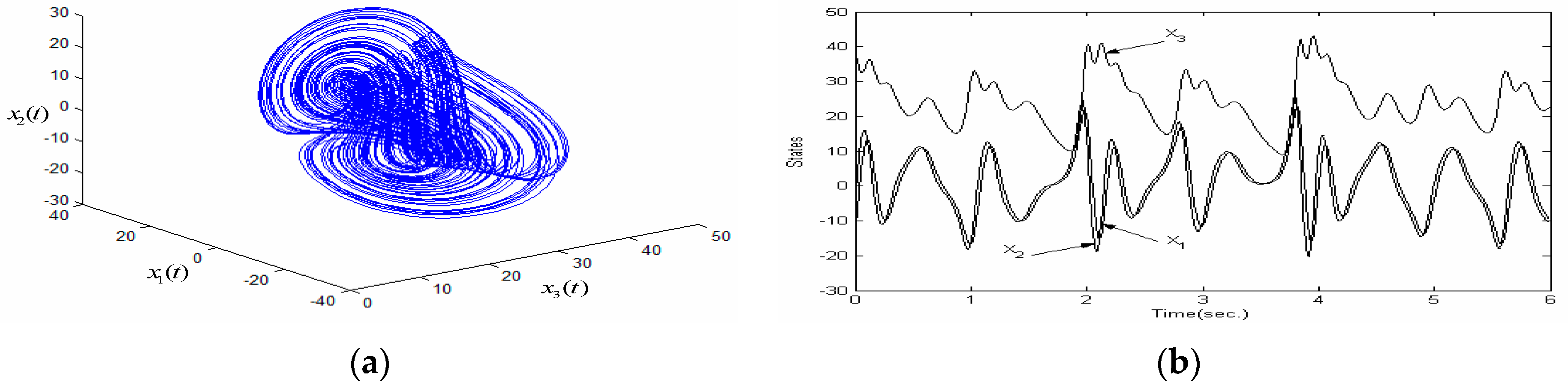
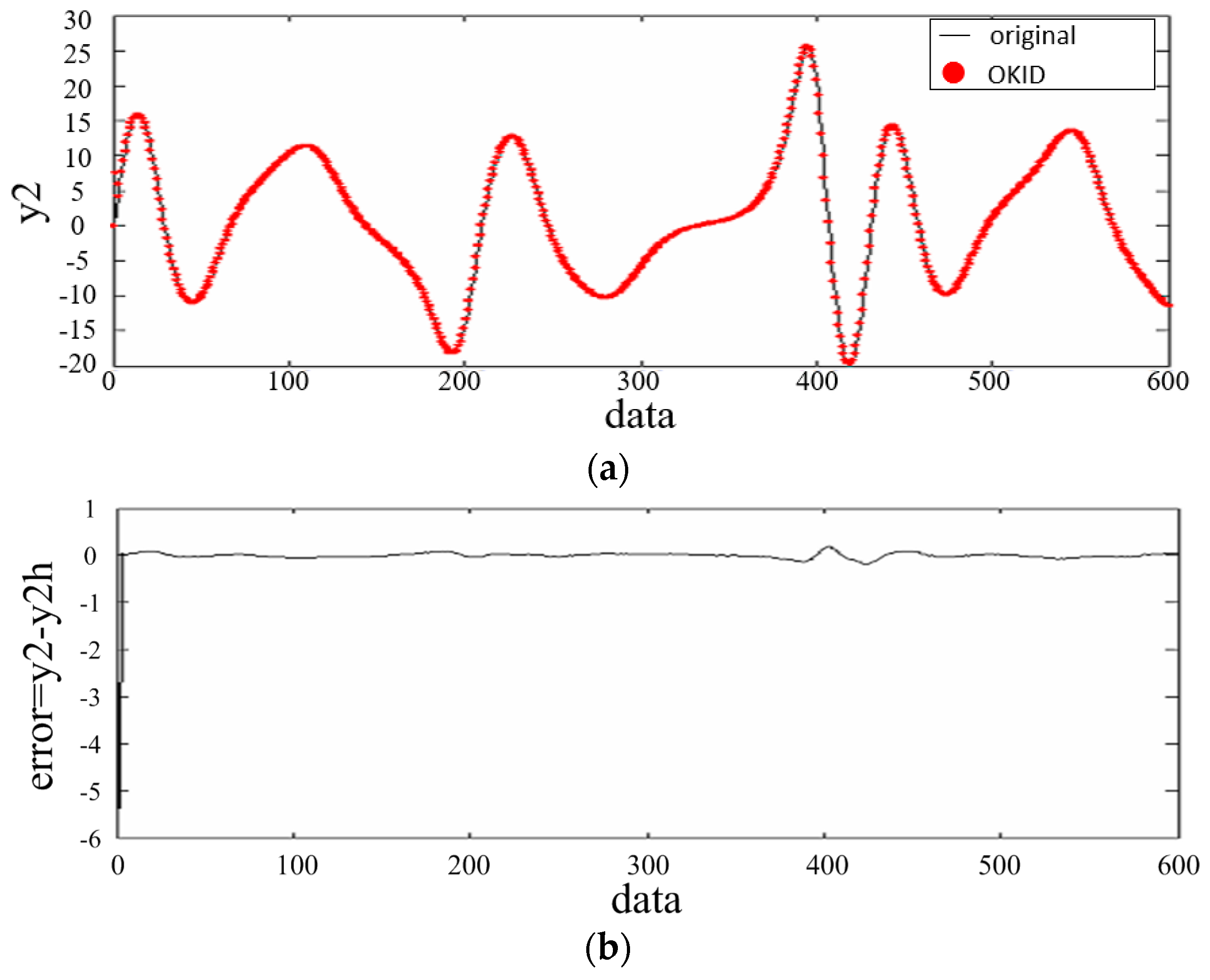
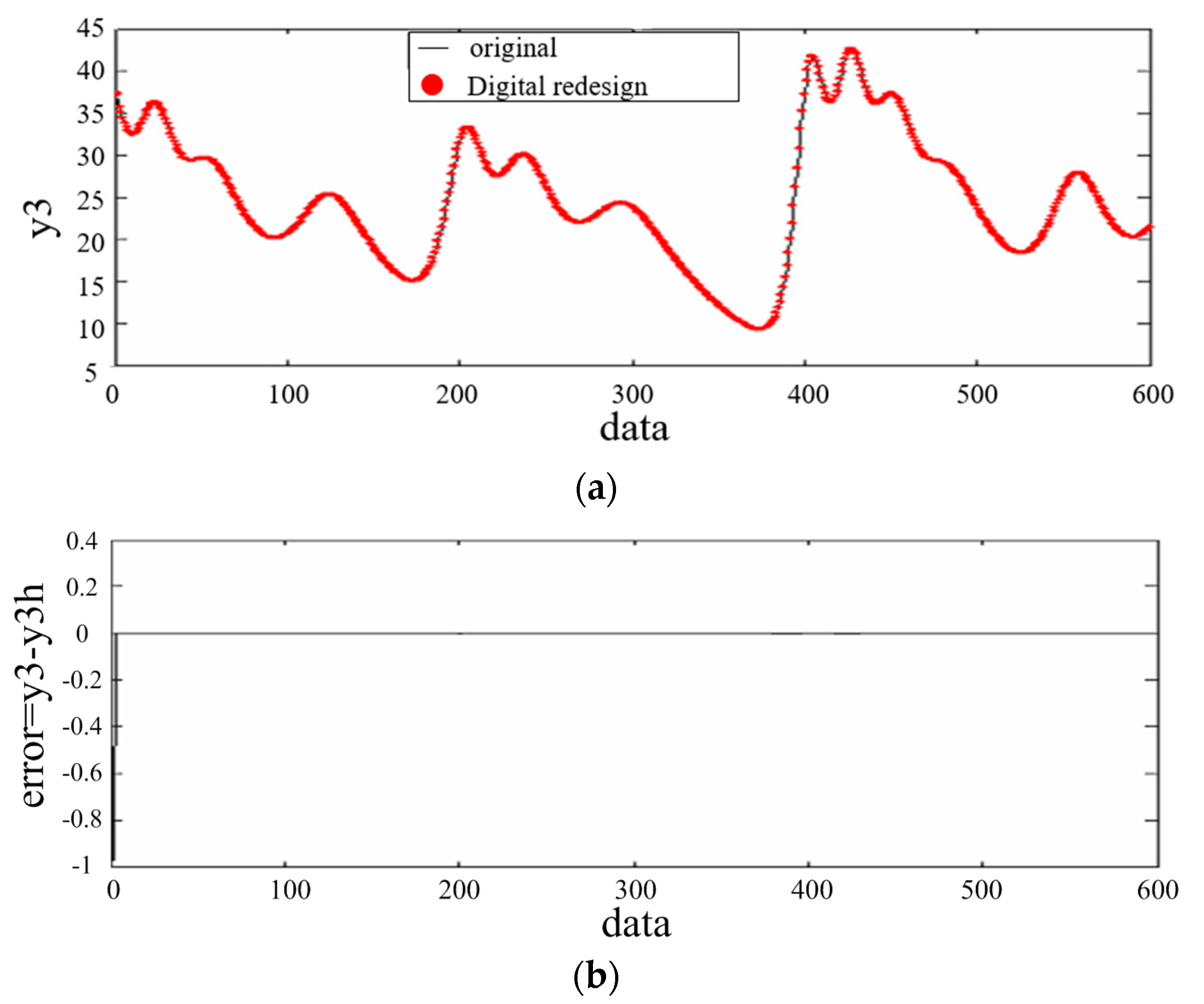
5. An Illustrative Example
Chen’s stochastic chaotic system is described by [10,11],
where the white noise process, , has zero mean and covariance; where for , nonnegative integer; the goal is to determine a sampling period for the computation of a piecewise constant signal. This system has the attractor and time series shown in Figure 3 where = 35, = 3, and = 28 without noises.
Figure 3.
(a) The deterministic chaotic attractor of Chen’s system, plotted in the space; (b) the deterministic chaotic time series of Chen’s system.
In the simulation, the sampling period = 0.005 s, final simulation time = 60 s, and initial conditions used are
Case 1: OKID Method
Based on OKID method, where , information data ; apply a singular value decomposition to to have and Then, compute system and observer-gain form in Equations (21)–(23) and matrices as
Finally, simulations of the stochastic chaotic trajectories of Chen’s system, and computation of observer Markov parameters are obtained, as shown in Figures 4a, 5a and 6a; and data of output error are shown in Figure 4b, 5b and 6b.
Figure 4.
(a) Trajectories of and ; (b) Data of output error .
Figure 5.
(a) Trajectories of and ; (b) Data of output error .
Figure 6.
(a) Trajectories of and ; (b) Data of output error .
Case 2: OKID Combined with a Digital Redesign Observer Method
Based on the new digitally redesigned observer form in Equation (38), the system and observer gain matrices are:
Finally, simulations of the stochastic chaotic trajectories of Chen’s system and computation of digital redesign observer parameters are obtained, as shown in Figures 7a, 8a and 9a, and data of output error are shown in Figures 7b, 8b and 9b.
Figure 7.
(a) Trajectories of and ; (b) Data of output error .
Figure 8.
(a) Trajectories of and ; (b) Data of output error .
Figure 9.
(a) Trajectories of and ; (b) Data of output error .
The error range of the outputs values (,,) of the OKID and OKID combined with a digital redesign method individually are shown in Table 1.
Table 1.
The error range of the outputs values (,,) of the OKID and OKID combined digital redesign method.
6. Conclusions
A new methodology of the OKID combined with an observer-based digital redesign tracker for a stochastic chaotic system has been proposed in this paper. The developed methodology was realized on Chen’s chaos system and showed the proposed method is about 10 times more accurate than the OKID-only algorithm. The main contributions of this paper are (i) A novel low-order observer-based digital redesign tracker for the equivalent chaotic system is theoretically possible to asymptotically track the stochastic chaos system with zero error; (ii) The developed scheme proposed speeds up the parameter identification process and could be utilized for on-line control system identification. In the future, we will extend this OKID combined with an observer-based digital redesign method to a variety of stochastic chaotic system controls.
Acknowledgments
This work was supported by the National Science Council of the Republic of China under contract MOST 104-2221-E-468-008-. The sponsorship period is 1 August 2015 to 31 July 2015. This fund is expired and could not ever support the costs to publish in open access.
Author Contributions
Tseng-Hsu Chien conceived and designed the experiments; Yeong-Chin Chen performed the experiments, analyzed the data, and wrote the paper.
Conflicts of Interest
The authors declare no conflict of interest.
References
- Juang, J.N.; Phan, M.Q.; Horta, L.G.; Longman, R.W. Identification of observer/Kalman filter Markov parameters: Theory and experiments. J. Guid. Control Dyn. 1993, 16, 320–329. [Google Scholar] [CrossRef]
- Ho, B.L.; Kalman, R.E. Effective construction of linear state-variable models from input-output data. In Proceedings of the 3rd Annual Allerton Conference on Circuit and System Theory, Monticello, IL, USA, 20–22 October 1965; pp. 449–459.
- Phan, M.; Horta, L.G.; Juang, J.N.; Longman, R.W. Linear System Identification via an Asymptotically Stable Observer; Technical Report NASA TP 3164; National Research Council, NASA Langley Research Center: Hampton, VA, USA, 1992.
- Juang, J.N.; Pappa, R.S. Effects of noise on modal parameters identified by the eigensystem realization algorithm. J. Guid. Control Dyn. 1986, 3, 294–303. [Google Scholar] [CrossRef]
- Juang, J.N. Applied System Identification; Prentice-Hall: Englewood Cliffs, NJ, USA, 1994; pp. 176–182. [Google Scholar]
- Chien, T.H.; Tsai, J.S.H.; Guo, S.M.; Chen, G. Lower-order state-space self-tuning control for a stochastic chaotic hybrid system. IMA J. Math. Control Inf. 2007, 24, 219–234. [Google Scholar] [CrossRef]
- Guo, S.M.; Shieh, L.S.; Chen, G.; Lin, C.F. Effective chaotic orbit tracker: A prediction-based digital redesign approach. IEEE Trans. Circuits Syst. I Fund. Theory Appl. 2000, 47, 1557–1570. [Google Scholar]
- Wang, H.P.; Tsai, J.S.H.; Yi, Y.I.; Shieh, L.S. Lifted digital redesign of observer-based tracker for a sampled-data system. Int. J. Syst. Sci. 2004, 35, 255–271. [Google Scholar] [CrossRef]
- Anderson, B.D.O.; Moore, J.B. Optimal Filtering; Prentice-Hall: Englewood Cliffs, NJ, USA, 1979. [Google Scholar]
- Chen, G.; Ueta, T. Yet another chaotic attractor. Int. J. Bifurc. Chaos 1999, 9, 1465–1466. [Google Scholar] [CrossRef]
- Yu, X.; Xia, Y. Detecting unstable periodic orbits in Chen’s chaotic attractor. Int. J. Bifurc. Chaos 2000, 10, 1987–1991. [Google Scholar] [CrossRef]
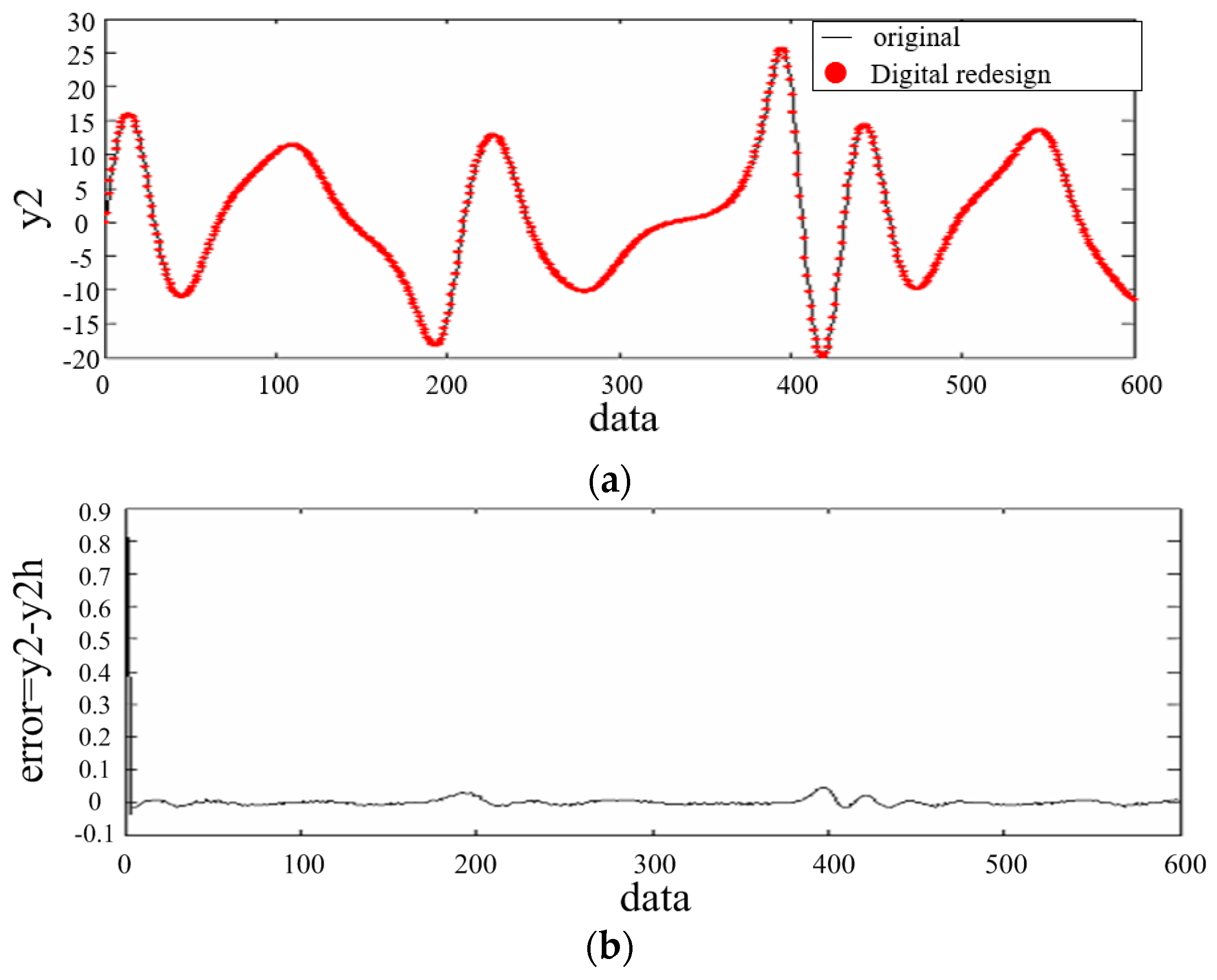
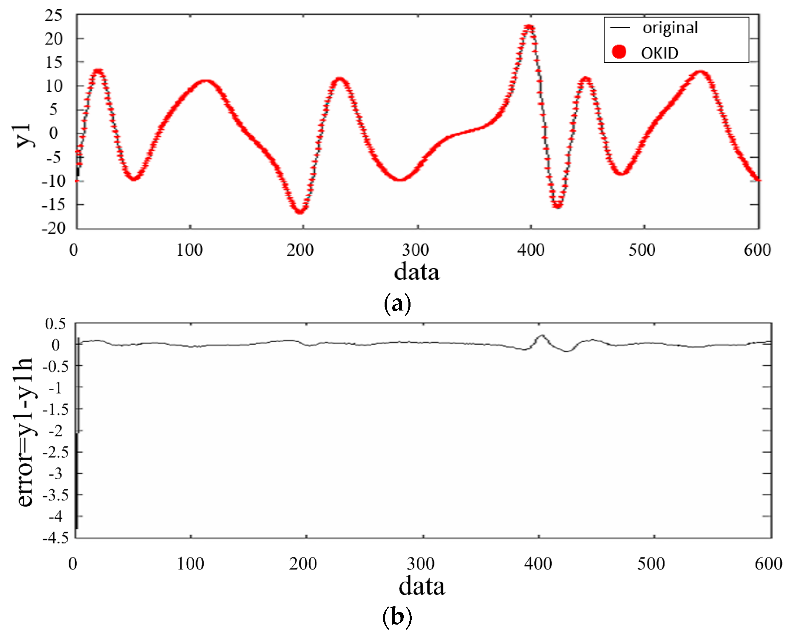
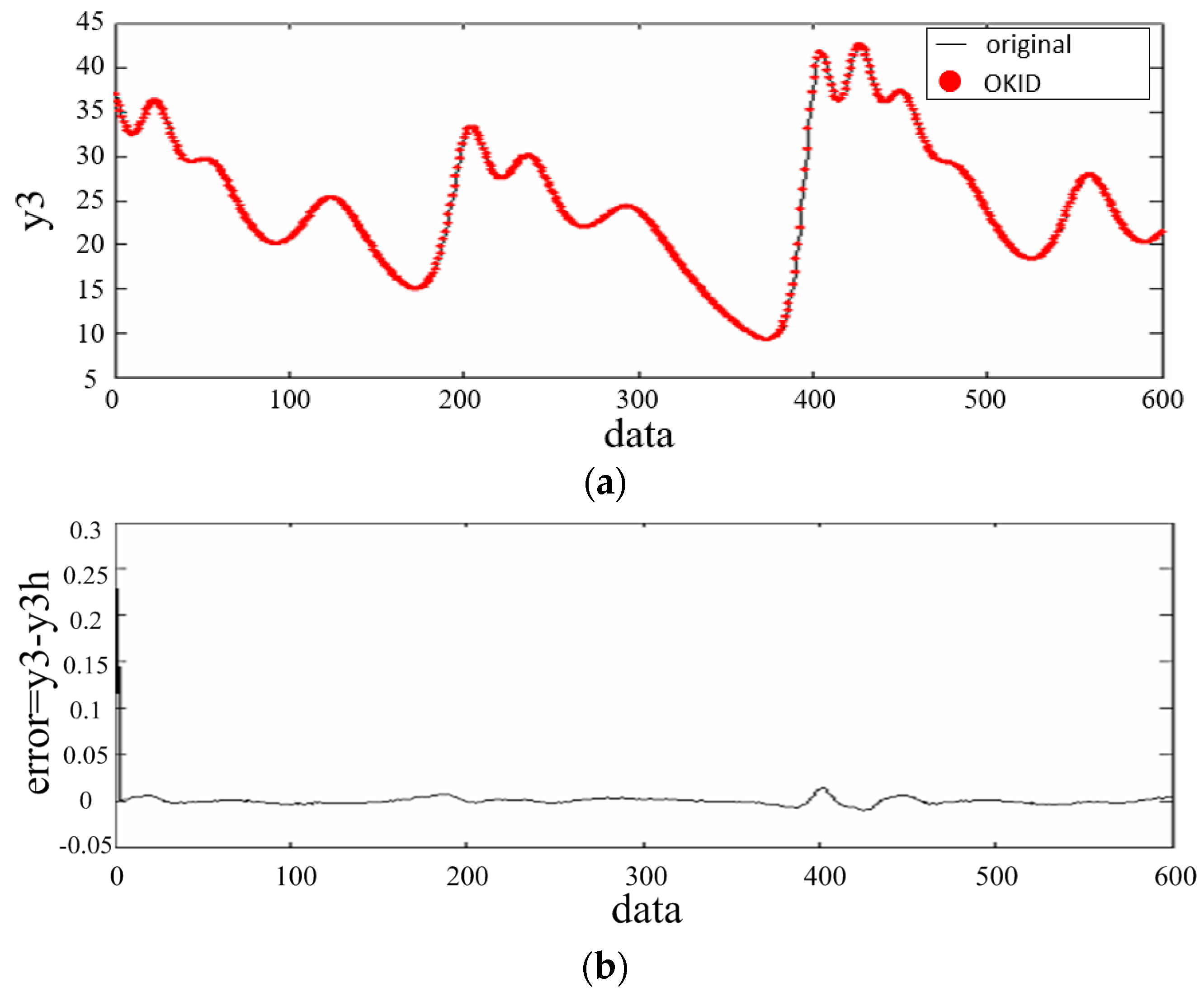
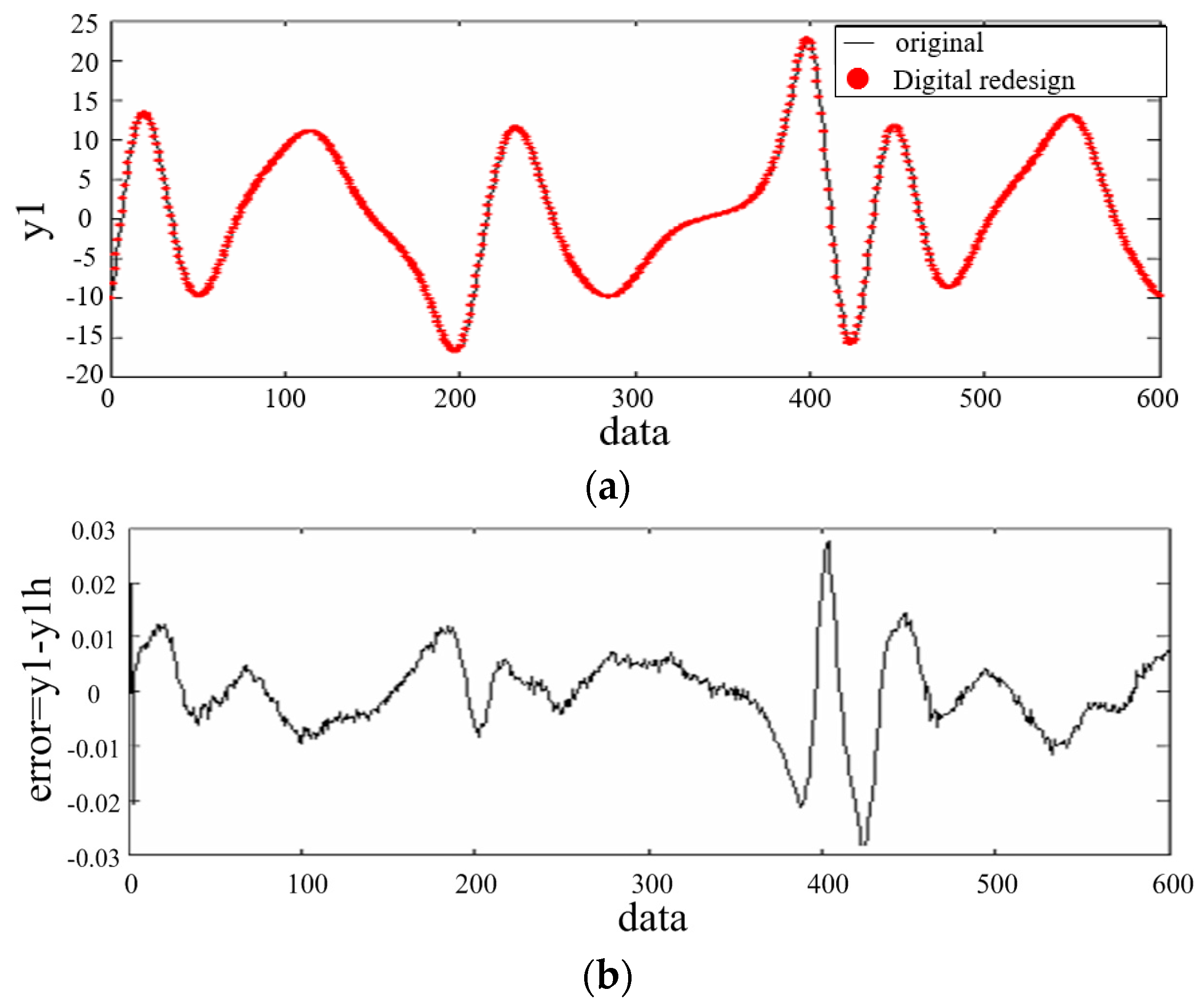
© 2017 by the authors. Licensee MDPI, Basel, Switzerland. This article is an open access article distributed under the terms and conditions of the Creative Commons Attribution (CC BY) license ( http://creativecommons.org/licenses/by/4.0/).