Abstract
This paper investigates a structured sparse SAR imaging algorithm for point scattering model based on tensor decomposition. Several SAR imaging schemes have been developed by researchers for improving the imaging quality. For a typical SAR target scenario, the scatterers distribution usually has the feature of structured sparsity. Without considering this feature thoroughly, the existing schemes have still certain drawbacks. The classic matching pursuit algorithms can obtain clearer imaging results, but the cost is resulting in an extreme complexity and a huge computation resource consumption. Therefore, this paper put forward a tensor-based SAR imaging algorithm by means of multiway structured sparsity which makes full use of the above geometrical feature of the scatterers distribution. The spotlight SAR observation signal is formulated as a Tucker model considering the Kronecker constraint, and then a sparse reconstruction algorithm is introduced by utilizing the structured sparsity of the scene. The proposed tensor-based SAR imaging model is able to take advantage of the Kronecker information in each mode, which ensures the robustness for the signal reconstruction. Both the algorithm complexity analysis and numerical simulations show that the proposed method requires less computation than the existing sparsity-driven SAR imaging algorithms. The imaging realizations based on the practical measured data also indicate that the proposed algorithm is superior to the reference methods even in the severe noisy environment, under the condition of multiway structured sparsity.
1. Introduction
Synthetic aperture radar (SAR) is a kind of radar system with the features of all-weather, multi-polarization and penetrability, which played a key role in remote sensing, detection and mapping fields in the past decades [1,2,3]. There are four common observation modes for SAR: Stripmap, Scan, Inverse and Spotlight [4]. Because the high resolution is conducive to capturing the structure information of the SAR targets, this paper focuses on Spotlight SAR. It is a beamforming-based observation technology, for which the radio beam will always point to the observation scene. The SAR image reconstruction is to acquire the scatter coefficients and to recover spatial distribution of the scatterers from the reflected waves. To obtain a better imaging resolution, a larger aperture will be synthesised by the coherent processing for the motions of targets relative to the antenna, as the pulse compression is usually applied on the range direction. However, in practical applications, traditional SAR imaging methods encounter many problems. Firstly, the receiver needs a higher sampling rate for the wideband waveform because of the Nyquist sampling limit, which leads to a considerable cost for data storing and processing. Secondly, the conventional techniques often suffer from the sidelobe disturbance which may lead to the performance deterioration of reconstruction, such as fuzzy in the SAR target image, etc.
Compressed sensing (CS) [5,6,7], as a novel theoretical framework appearing in literature recently, can obtain necessary information via sub-Nyquist sampling rate for sparse signal, which can reduce storage requirement and simplify the design of hardware system. That is why CS has attracted greater attention in SAR imaging. In 2001, Cetin et al. introduced the sparse constraint into spotlight SAR imaging, and proposed a method to improve the target feature [8]. CS was first applied in super-resolution radar imaging by Baraniuk et al. in 2007, and a new type of radar system was proposed based on sparse reconstruction [9]. In 2009, Gurbuz et al. analyzed the application of sparse reconstruction in ground-penetrating radar imaging, and proposed a sparse imaging algorithm based on -norm minimization [10]. In the next year, a SAR imaging method based on sparse reconstruction theory was introduced by Potter et al. [11], which can achieve a higher reconstruction resolution than the traditional imaging methods. In 2011, the effect of parameter selection of SAR imaging based on regularized sparse reconstruction was studied by Batu et al. [12]. In order to accelerate the speed of SAR imaging algorithm, a sparse regularization technique based on iterative threshold method was proposed by Fang et al. in 2014 [13]. For moving targets, Zhang et al. proposed an efficient SAR imaging method in 2015 [14] combining fractional Fourier transform technology with CS framework. However, these studies dealt only with the spatial sparsity of the observation without exploiting the structural characteristics of scatterers in the target scene. In practice, the imaging results show that the scatterers tend to be aggregated together as clumps. The sparse reconstruction schemes have ability to accomplish SAR imaging based on object-level information of scatterers and possess the robustness to noise [15]. In 2016, Zhao proposed a CS-based SAR imaging algorithm with structured sparsity constraint, in which a hierarchical Bayesian learning framework was applied [16]. Since hierarchical model is designed, the requirement for model matching of such kind of algorithm is strict, thus the imaging quality may deteriorate once observation data is mismatched with the model.
To solve the above problems, we introduce a tensor decomposition algorithm in this paper both to reap the model robustness and to lower resource requirement. The real-world signal is usually multidimensional and structured. In order to deal with such higher-order data processing problem, tensor decomposition is studied widely. For instance, tensor modeling is utilized in chemometrics to analyse spectroscopy [17], and is also applied to acquire two-dimensional direction of arrival (DOA) estimation by taking advantage of the Vandermonde structure in array manifold [18,19]. For SAR imaging problems, tensor modeling is capable of exploiting the structured sparse distribution of the scatterers to gain more robustness. Because of the curse of dimensionality in higher-order data processing [20,21,22], making use of the sparsity is becoming a research hotspot in recent years. In 2010, Lim and Comon applied tensor decomposition to propose a sparse reconstruction method, and derived the uniqueness condition of tensor decomposition [23]. Duarte et al. first introduced the Kronecker constraint into the construction of dictionary in 2011, and proposed the Kronecker-CS model [24]. In low rank tensor signal processing, Sidiropoulos et al. introduced the CS theorem into a two-step sparse signal reconstruction algorithm in 2012 [25]. The following year, Caiafa and Cichocki proposed two types of matching pursuit algorithms based on tensor model incorporating with CS method [26]. Although there has been little public research about combining sparse representation with tensor decomposition in SAR imaging field, potential advantages of this method with robustness and efficiency inspire us to apply it in solving the open problems. The application of higher-order CS in image processing, such as hyperspectral imaging [24,27] provides the inspiration of this work, but this is still in the stage of preliminary study. We formulate the SAR echo signal as a Tucker model based on its Kronecker information and then construct a sparse reconstruction algorithm by utilizing the structured sparsity of target scene. Both the theoretical analysis and numerical experiment verifications reveal that the proposed algorithm is superior to the existing methods, such as spatially variant apodization (SVA) [28,29] and matching pursuit algorithms [30,31,32].
The following is the organization of other sections in this paper: Section 2 describes the received signal model of SAR imaging and its tensor modeling; Section 3 constructs the algorithm based on Kronecker constraint and multiway structured sparsity of the signal model; Section 4 provides several groups of numerical experiments to verify the proposed method, and compare with the existing methods in performance; Section 5 concludes this paper.
2. The Tensor Modeling of Structured Sparse SAR Imaging
2.1. Received Signal Model
For convenience of statement hereafter, several notions of this paper are explained as follows. The scalar is indicated by italic letter, e.g., s; the vector and matrix are indicated by bold italic letters, e.g., ; the tensor is indicated by calligraphic capital letter, e.g., ; the index of a set is indicated by script letter, e.g., .
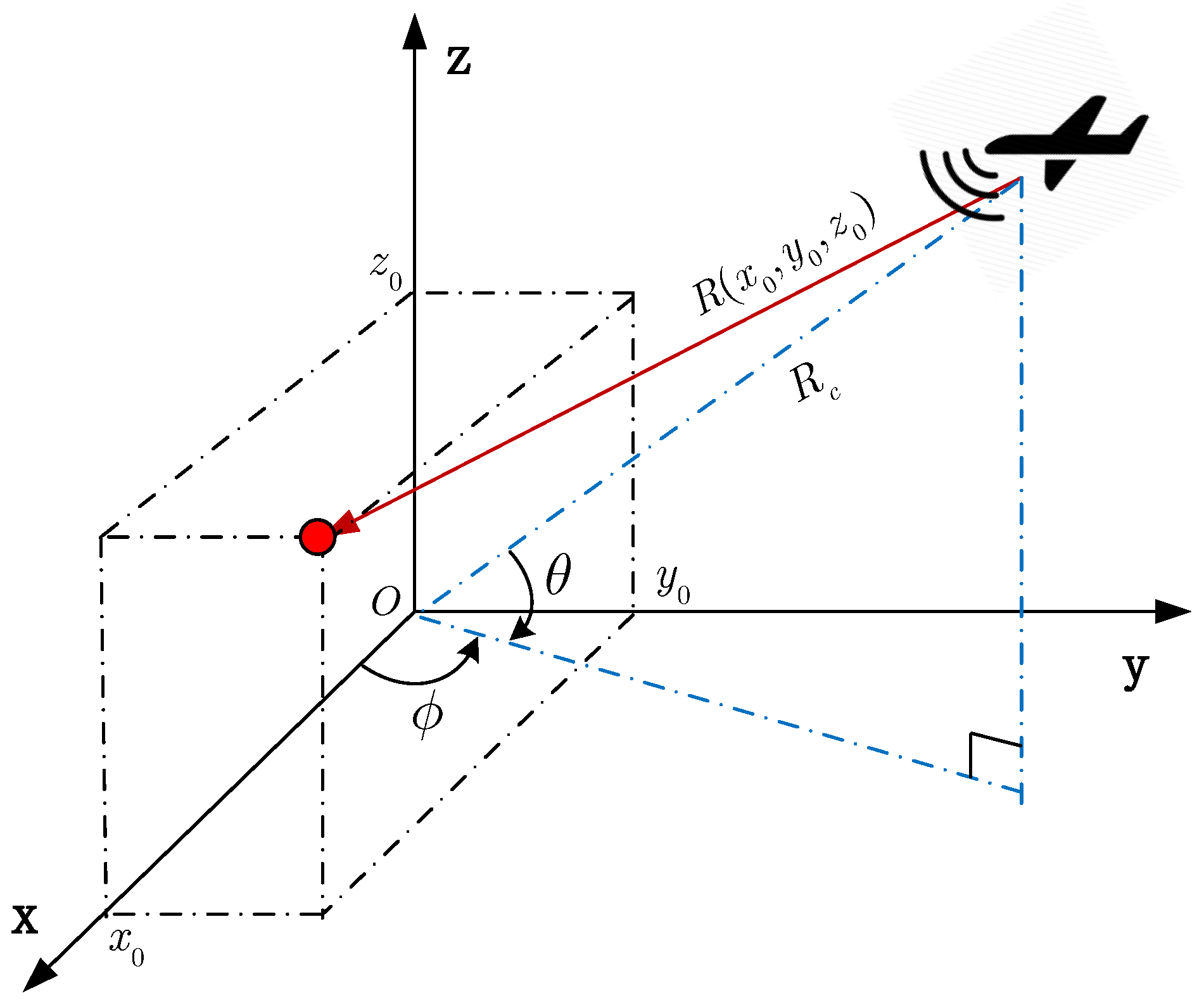
Here we consider the point-scattering models [3]. The spotlight SAR geometry is illustrated in Figure 1. The target scene is represented by coordinate system. The azimuth and pitch angles of antenna relating to the center of the scene are ϕ and θ. The distance between target and antenna is , where denotes the distance between the antenna and the center of target area. The time delay for the target point in SAR echo signal is , where c is the speed of light.
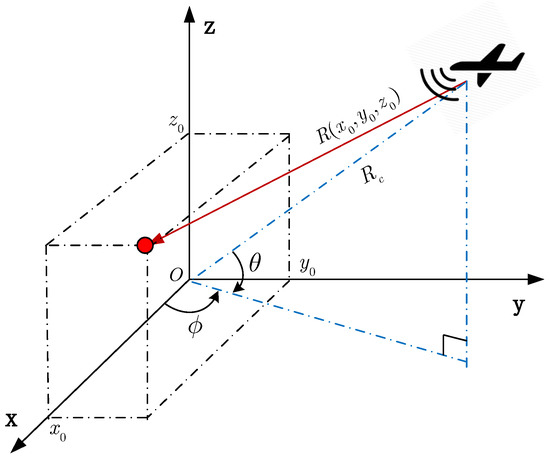
Figure 1.
The geometry of spotlight SAR for point scatterers.
After matched filtering, the reflection signal is
where is the scattering function of scatterer placed at ; is the autocorrelation function of transmitted signal; is the additive noise. In the following discussion the noise is neglected for notational simplicity. Then the phase history can be obtained through Fourier transform:
where can be ignored as it is a constant for all scatterers, and the phase factor is .
For decoupling between the parameters in the phase factor, an interpolation approach is applied and the polarization coordinates is transformed to a Cartesian coordinates [33]. Assume there are grid points along the directions of the axis of x, y, z, respectively; and the number of grid points for are , respectively. Then for the scatterer at , the steering vector is , where . Let . Define the steering matrix as
then the received signal model (2) can be rewritten as
where .
2.2. Kronecker Dictionary
For a vector signal , we consider that a K-sparse representation is existed on a dictionary , if the following relationship is satisfied:
where is the -norm of , indicating the number of nonzero elements in ; K is defined as sparsity. Usually, .
Because the number of rows is less than the columns, this is a underdetermined system which means there is no unique solution of . However, a sparse solution can be obtained if the signal has the feature of sparsity and the following condition is satisfied [30]:
where , indicating the coherence coefficient of dictionary .
If the dictionary has Kronecker constraint, i.e., , the coherence coefficient can be defined as
where . It is shown from (9) that for a Kronecker dictionary, the overall coherence depends merely on the factor matrix with the greatest coherence [34].
The previous studies [35,36] indicated that, for the signal recovery problem with the same sparsity level, the reconstruction procedure based on Kronecker dictionary has much less strict requirements for coherence than the classic matching pursuit method. In other words, the former has the higher recovery bound [26]. In addition, by using the structural information of signal, the reconstruction algorithm based on Kronecker dictionary performs robustly under the condition of high coherence.
2.3. Multiway Sparsity
One-dimensional expansion of a tensor is defined as stacking all elements along the mode-1, e.g., , where mode is considered as the order of a tensor. Then the Tucker decomposition of is expressed as , where denotes the mode-n product of tensor with matrix [37], which can be written as
It is indicated from (10) that a Tucker decomposition of a multiway data is equivalent to a linear representation with Kronecker dictionary.
Definition 1 (Multiway sparsity).
If in the Tucker model (10) is K-sparse with respect to , then is K-sparse with respect to the factor matrices . The columns of are the atoms along each mode.
For an N-dimensional signal, if it has a K-sparse representation, the core tensor of Tucker decomposition has K nonzero elements, i.e.,
where "∘" is the outer product operator. Because the nonzero entries of scatter coefficients are non-uniformly distributed and always gather together in the practical application of SAR imaging, this feature results in the highly structured echo signal, by which more rapid algorithm may be constructed.
Definition 2 (Multiway structured sparsity).
A multiway signal is called -structured sparse, if the factor matrices of its Tucker decomposition only need columns to compute, i.e.,
where indicates a subset of the indices for mode-n.
By Definition 2, the nonzero elements of core tensor are concentrated in a subtensor . Then the relationship between multiway structured sparsity and the vector signal sparsity can be deduced: is K-sparse () with respect to Kronecker dictionary . It should be noted that the definition of structured sparsity here is different from the definition of block sparsity used for one-dimensional signal. For the latter, a coefficient vector is called block K-sparse if it consists of a series of concatenate segments, named blocks, and the number of segments without nonzero Euclidean norm is less than K [38,39].
3. The Proposed Method
3.1. Sparse Reconstruction Based on Kronecker Dictionary
Compressed sensing can reconstruct the source signal from the undersampled measurements. Applying the technique to SAR super-resolution imaging still faces many challenges. The sparse imaging method is mainly to solve an ill-posed linear inverse problem by using the sparsity of radar cross section (RCS). For the large scale data, the classic procedure will be rigorously challenged by many computation problems. For instance, considering a scene with observation points, the classic reconstruction approach will deal with data in length up to 1048576, which leads to a tremendous linear system, consuming computation resource significantly. From the analysis above, it is known that the target scene has the sparsity and the scatterers usually clustered together to blocky areas. Therefore, considering the structured sparse feature, the SAR imaging can be treated as a sparse reconstruction problem with Kronecker dictionary. A multiway structured sparse matching pursuit algorithm can be constructed to estimate the scatter coefficients with much fewer iterations.
Firstly, the SAR echo signal must be decoupled, for which the tensor data , and dictionaries along each mode have to be constructed. Our purpose is reconstructing the nonzero scatter coefficients from , i.e., finding a -structured sparse representation corresponding to . Because of the sparsity of target scene, only a fewer rows need to be randomly extracted from the dictionary.
Let , and then the Tucker decomposition of the original signal can be rewritten as
where is the vectorization of all nonzero elements. Consequently, the solution of the problem can be described as
Defining , the solution of (14) can be written as . Efficient calculation steps can be deduced by Cholesky decomposition [40].
| Algorithm 1 Tucker decomposition based SAR imaging algorithm. |
|
In iterative process, make sure that the nonzero elements of core tensor are always contained within a small index set. Finally all the nonzero elements and the corresponding index set are obtained and the expected scatter coefficients can be recovered as well. The algorithm flow is represented in Algorithm 1.
3.2. Algorithm Complexity Analysis
The first step of iteration needs to calculate , and the corresponding computational cost is . In addition, the absolute maximum optimization should be calculated, which needs operations. Comparing with this, the classic matching pursuit method, such as orthogonal matching pursuit (OMP) [30,32], requires the computation cost in this step.
With the application of the Cholesky decomposition, the computational complexity of estimating can be reduced efficiently in the iteration. Even if every mode need to be updated, the total computational cost can not exceed . By comparison, the computational cost of OMP algorithm is in this step.
In the residual calculation step, it is needed to compute and subtract it from . The corresponding calculations are . The ones of the OMP algorithm in this step, by contrast, are .
With regard to iterations, for a -structured sparse problem, the maximum iterations is . But OMP algorithm needs times iteration for the same problem.
4. Numerical Simulations and Discussion
This section will demonstrate several experiments to verify the proposed method. The simulations are classified into two parts, one is spotlight SAR imaging realization, including ideal point-scatterer target setting and real data experiments; the other is performance comparisons between the proposed algorithm and the existing methods, including error curves and computational cost. We choose three algorithms as references: SVA [28], OMP [30] and compressive sampling MP (CoSaMP) [31].
The SVA algorithm is a kind of apodization filtering SAR imaging method, which is designed to achieve sidelobe control. However, the performance of such classic algorithm is susceptible by noise, and the resolution is limited, especially for adjacent targets. Both OMP and CoSaMP belong to sparse reconstruction algorithms, which have the advantage of super-resolution due to the robustness to sidelobe disturbance and noise. The hardware configuration for the simulation system is: Intel Core i7-5500U 2.4 GHz, 8 GB RAM, Windows 10.
4.1. Realization of SAR Imaging
In this section, two groups of simulation experiments are presented to verify the effectiveness of the proposed method. One investigates the SAR imaging of ideal point targets and the other considers the practical measured data. The simulation scenario is stated as Table 1.

Table 1.
System parameters setting for spotlight SAR.
4.1.1. SAR Imaging for Ideal Point Targets
This section includes two settings of simulations: The first group investigates the imaging results via modifying the signal-to-noise ratio (SNR) under the condition of fixed number of scatterers. The second one inspects the imaging resolution via changing the the number of scatterers with fixed SNR.
(1) Different SNRs
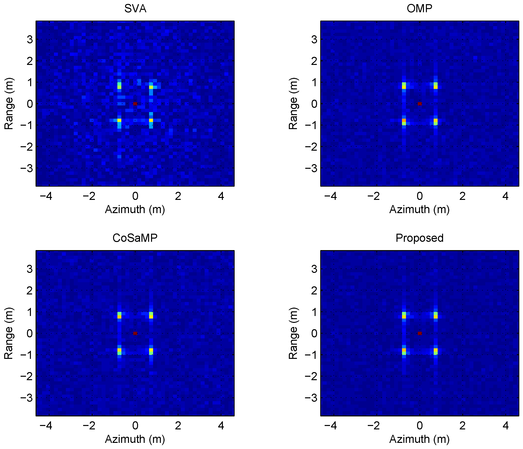
We investigate the effectiveness of the proposed method according to different noise conditions, from the low to the high SNR configurations. Five ideal point scatterers are placed around the centre of target scene in this simulation scenario.
The Figure 2 and Figure 3 show the SAR imaging realizations at the situation of the 3 dB and 30 dB SNR, respectively.

Figure 2.
SAR imaging simulation for ideal point scatterer model (SNR = 3 dB).
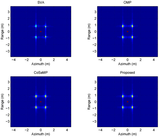
Figure 3.
SAR imaging simulation for ideal point scatterer model (SNR = 30 dB).
These two simulations demonstrate the imaging quality of the proposed method. For the low SNR, the imaging result of SVA shows severe ambiguity owing to the noise instability of this procedure. In comparison, the proposed algorithm performs much better, and the two matching pursuit algorithms also show good results. For the highest SNR, the imaging quality of all algorithms approach to the same.
(2) Different number of scatterers
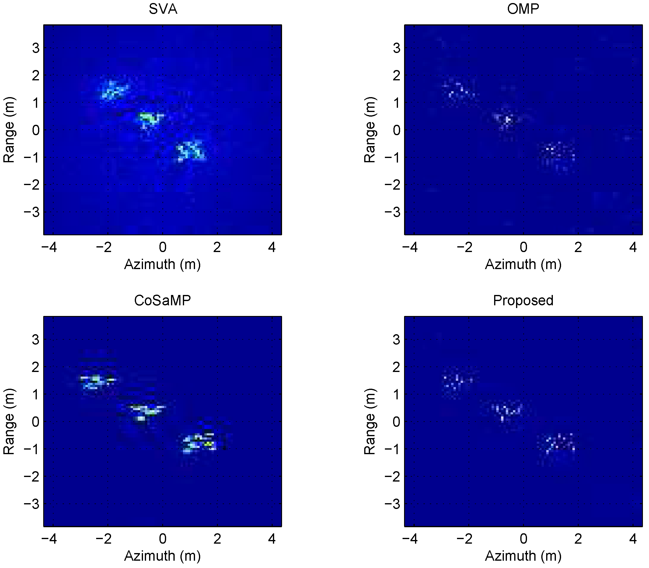
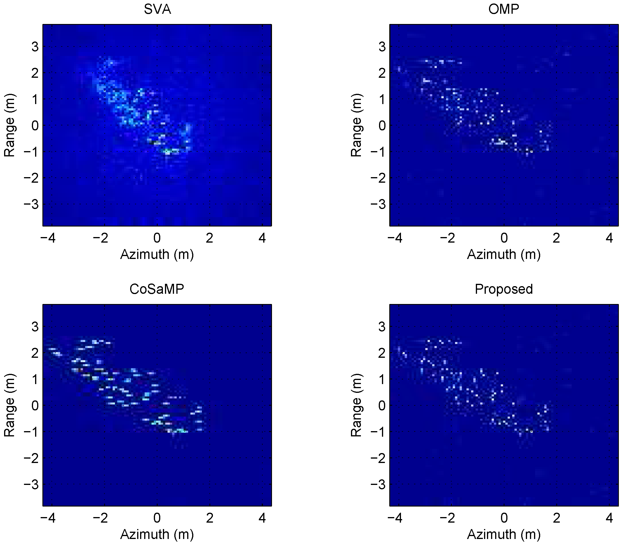
In this simulation scenario, the SNR is fixed at 5 dB. All the scatterers are gathered around three target clumps and such scatter centers are distributed along the diagonal line of the scene.
At the situation of scatterer number being 30, the SAR imaging realizations are shown in Figure 4. When the number of scatterers is set to 150, the SAR imaging realizations are shown in Figure 5.
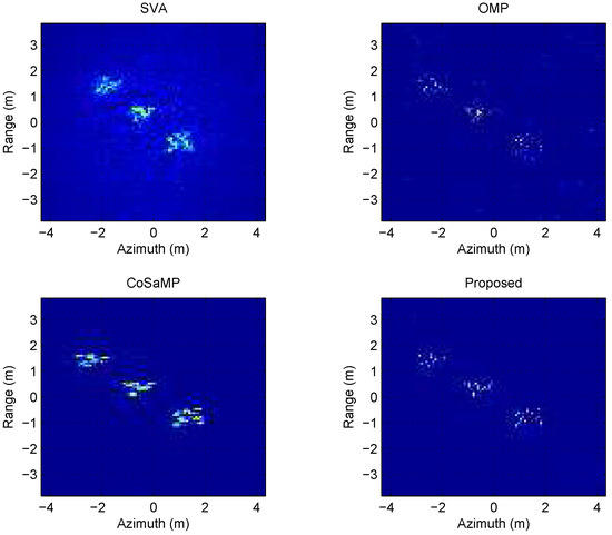
Figure 4.
SAR imaging simulation for ideal point scatterer model (30 scatterers).
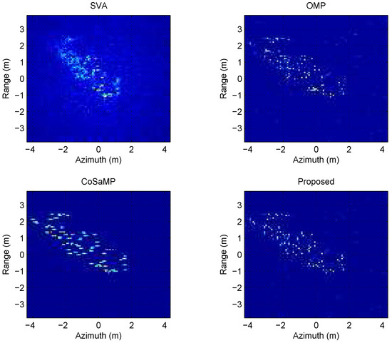
Figure 5.
SAR imaging simulation for ideal point scatterer model (150 scatterers).
From the two groups of simulations above, it is indicated that for the small number of scatterers, all the methods are able to reconstruct target scene well. Compared with SVA, the sparse-reconstruction-based methods obtain more explicit images. It is worth noting that simulation results of the proposed method contain few noisy points. As the scatterer number increases, the scatterers imaging results appear fuzzy. Under the same scenario, the reconstructed scene of the proposed method achieve the most accurate images.
4.1.2. SAR Imaging for Practical Measured Data
This group of experiments deal with real data, measured by a spotlight SAR. The observed target is a crawler-type vehicle. The radar data are obtained from different azimuth and pitch angles. The angle aperture is . The center frequency is 9 GHz and the bandwidth is 1 GHz. The number of observation angle samples and frequency samples are both set to 101, thus the number of total pixels of image is .
The matrix is constructed as the indication of the Equation (3), and rows are extracted from it to form a projection matrix. Here, is taken. Note that the number of observations , where K is the sparsity. Therefore, the sparsity can be expressed as . K is designed as 200 in this experiment.
In the following, we investigate the results at different azimuth angles under the condition at a fixed pitch angle firstly, and observe the results at different pitch angles under the condition at a fixed azimuth angle secondly.
(1) Different azimuth angles
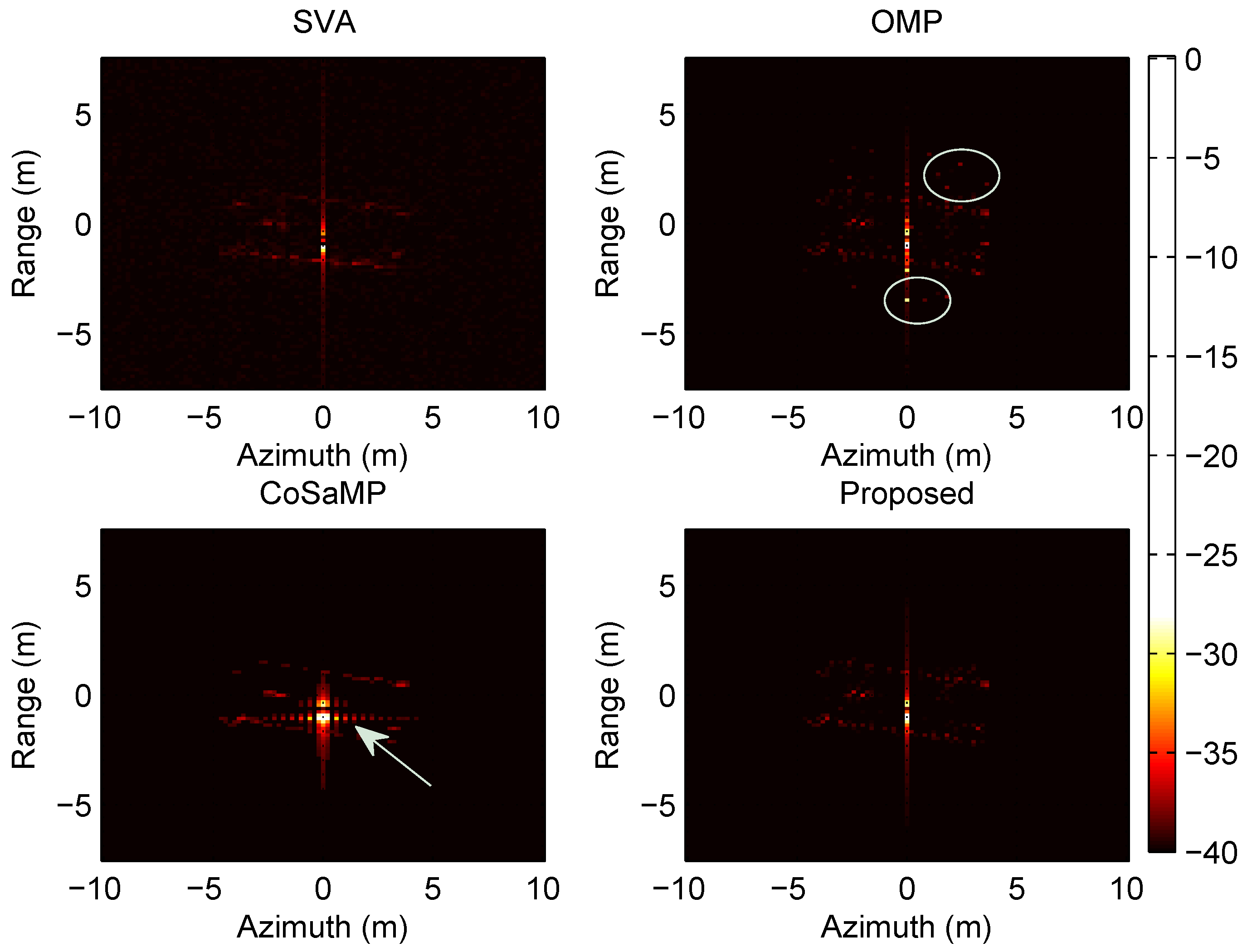
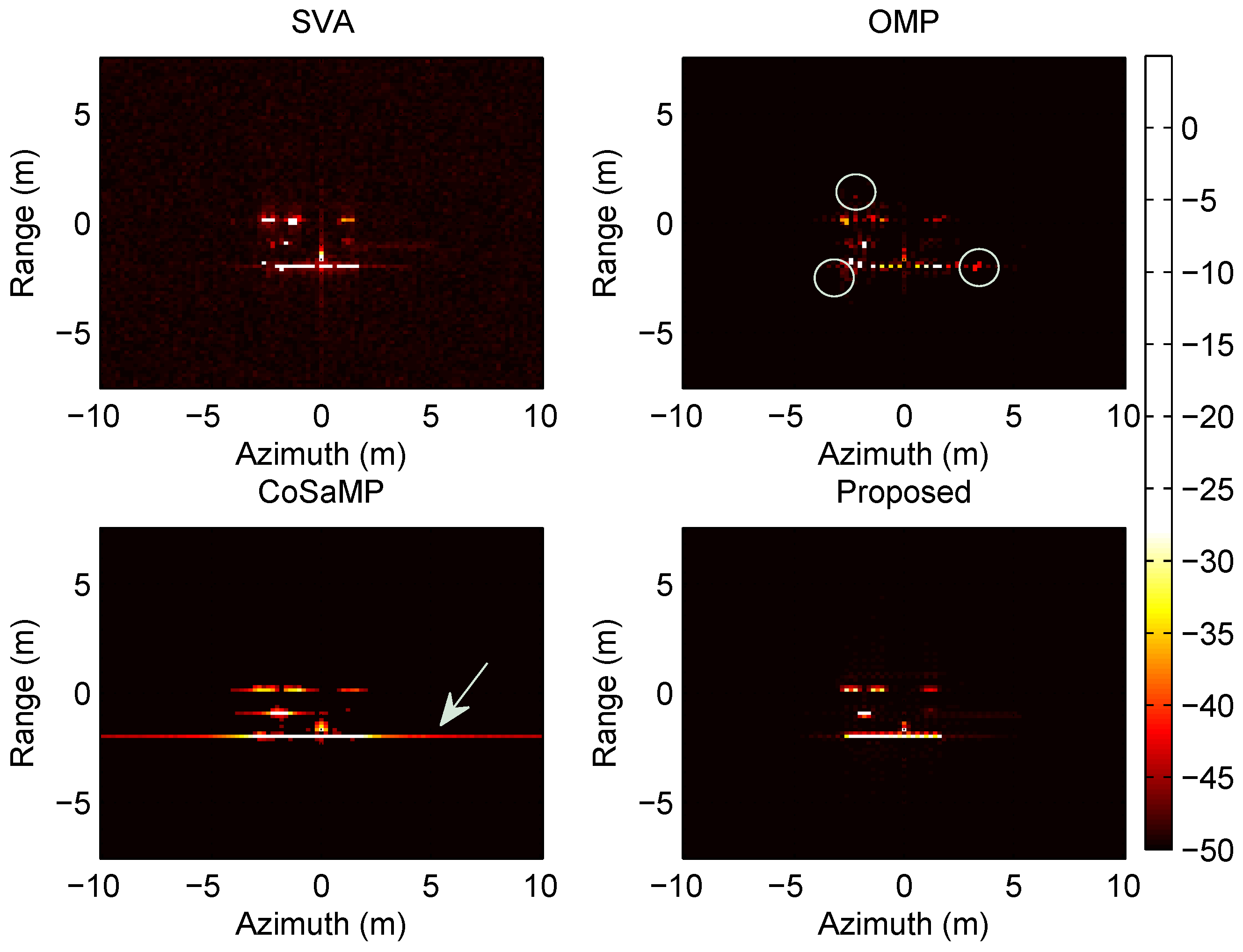
The pitch angle is fixed at . The observation data are acquired from three azimuth central angles, , and , respectively. And the corresponding SAR imaging realizations are shown in Figure 6, Figure 7 and Figure 8, respectively.
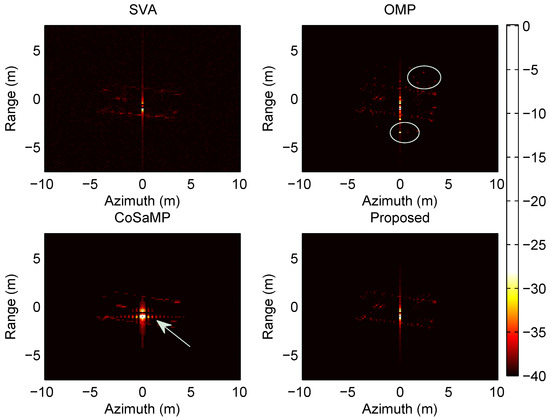
Figure 6.
SAR imaging for practical measured data, .
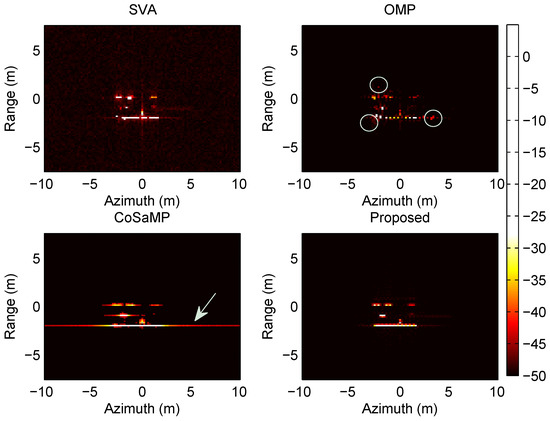
Figure 7.
SAR imaging for practical measured data, .
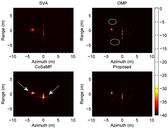
Figure 8.
SAR imaging for practical measured data, .
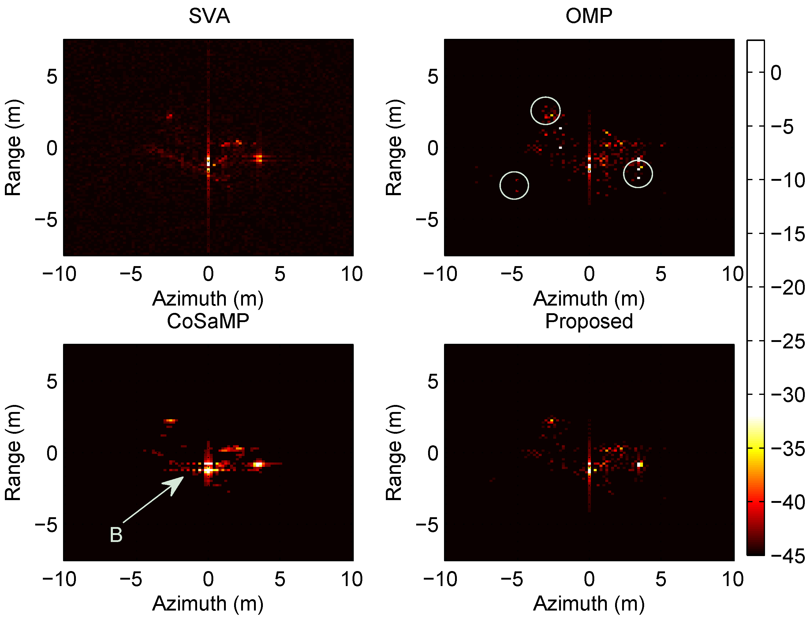
The above experiments demonstrate the effectiveness of the proposed method in practical implementation. With the comparison between the selected algorithms, the proposed method obtains the better imaging results. When the azimuth central angle is , the imaging result of SVA is dim and blurred, but the vehicle contour is clearly visible with the proposed method. For the experiments of different azimuth angles, although the classic matching pursuit approaches, i.e., OMP and CoSaMP, perform much better than SVA, the problem of imaging target ambiguity still exists. For instance, the CoSaMP imaging result has a remarkable bright streak at of the azimuth central angle, as shown in Figure 7. Besides, as indicated by the arrows in Figure 6 and Figure 8, CoSaMP shows raster lines over the target image at the central region, which will disturb the recognition of targets significantly. Under the same scenario, there exist incorrect scattering points on the sides of the target in the OMP imaging results, which are circled in white for each images. By contrast, the proposed method does not have such problems in all the experimental tests.
(2) Different pitch angles
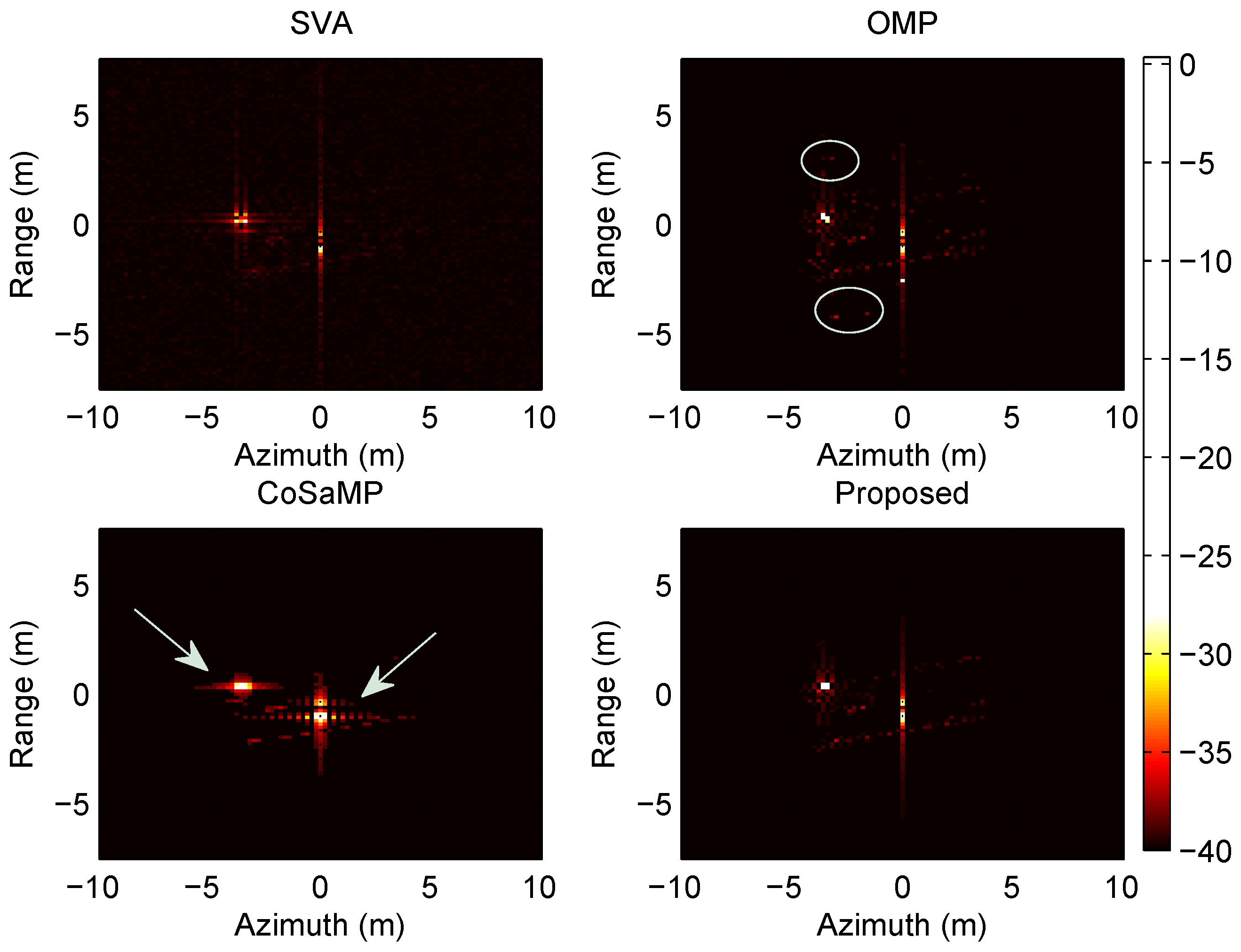
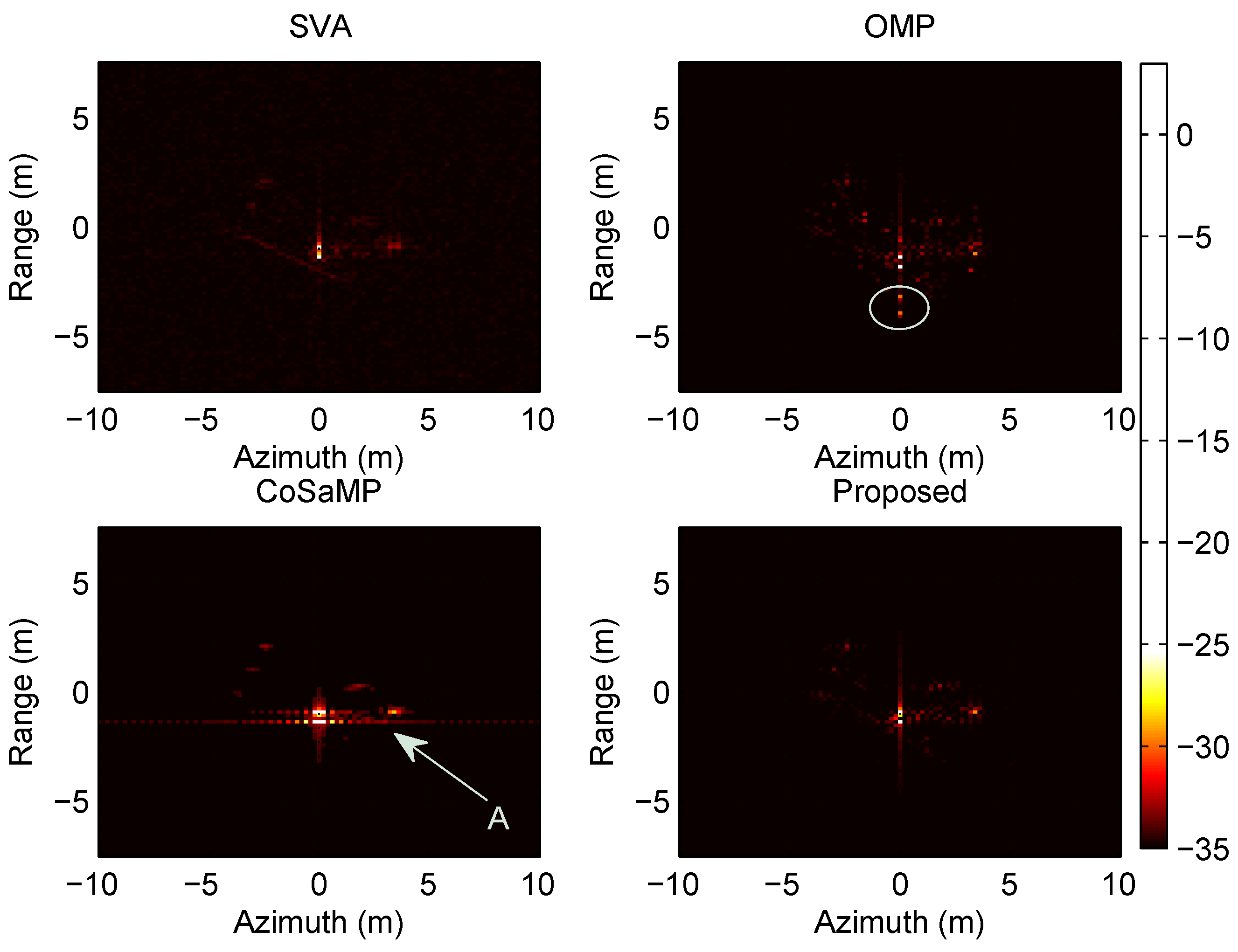
The azimuth angle is fixed at . The observation data is obtained from three pitch angles, , and , respectively. And the corresponding SAR imaging realizations are shown in Figure 9, Figure 10 and Figure 11, respectively.
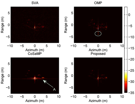
Figure 9.
SAR imaging for practical measured data, .
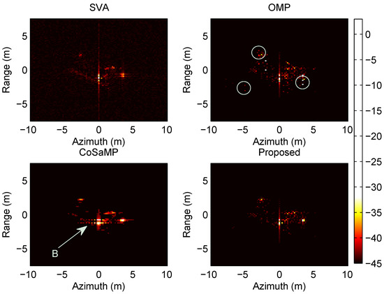
Figure 10.
SAR imaging for practical measured data, .
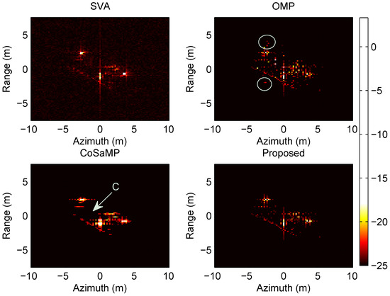
Figure 11.
SAR imaging for practical measured data, .
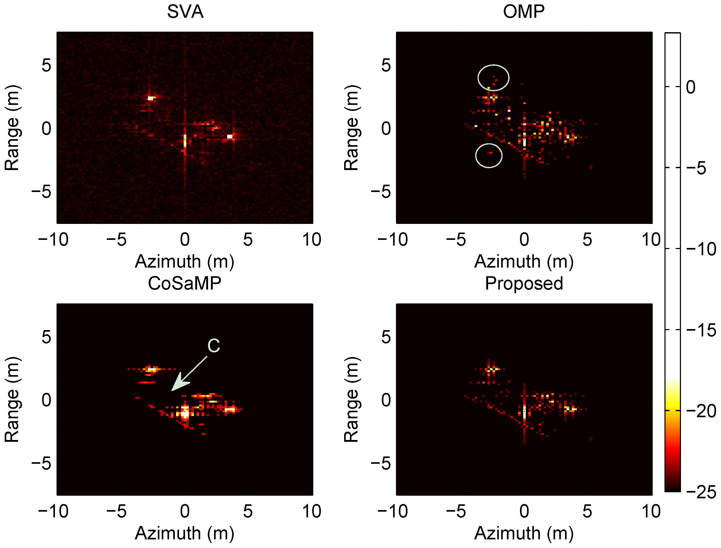
With the comparison between the experiments of different pitch angles, the superiority of the proposed method is demonstrated. As shown in Figure 11, the imaging result of SVA contains many noisy points appearing blurred; OMP outputs several outliers which are marked by white circles; for CoSaMP, a part of the scatter points in the central are lost, which is indicated by arrow C; but the proposed method obtains the clear and accurate imaging result. As shown in Figure 9 and Figure 10, the imaging results of CoSaMP contain raster lines over the targets which are indicated by arrow A and B, respectively; the other three methods achieve the similar performance as demonstrated above. Although the two classic matching pursuit methods can obtain clearer images than SVA, but both of them result in errors of the estimation beyond tolerance. By contrast, the proposed method can achieve the better imaging results. This is true especially as the pitch angle increases.
4.2. Performance Comparison
This section focuses on two performance indicators of the proposed method and the reference methods, one is the root mean square error (RMSE) curve, the other is the computational resource requirements.
4.2.1. RMSE
The RMSE of SAR imaging model is defined as follows:
where is the estimate of scatter coefficients in the lth Monte-Carlo independent trial.
(1) Different SNRs
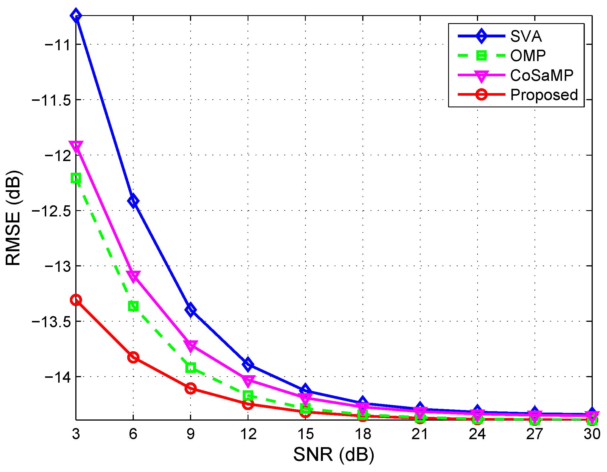
The configuration of this experiment is the same as Section 4.1.1. The SNR range is 3∼30 dB, and L, the number of independent trials, is set to 500. The RMSE curves are shown in Figure 12.
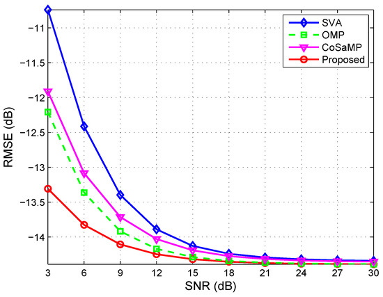
Figure 12.
RMSE comparison versus different SNRs (, , ).
It is demonstrated from the RMSE curves that the performance of the proposed method is better than the others under the condition with low SNR. As the SNR increasing, the RMSE curves of the reference methods are approximately approaching to the one of the proposed method. Because of the sensitivity to noise, the reconstruction error of SVA algorithm is considerable in low SNR. In this respect, the sparse-reconstruction-based methods are robust to noise. The simulation results show that the performance of CoSaMP is slightly worse than that of OMP. The reason is that CoSaMP only chooses atoms at each iteration, which can help to improve the efficiency of the algorithm, but may reduce the success rate of reconstruction. In comparison, the proposed method performs much better, even if the noise interference is serious. This is because the Kronecker information of the echo signal is fully utilized.
(2) Different number of scatterers
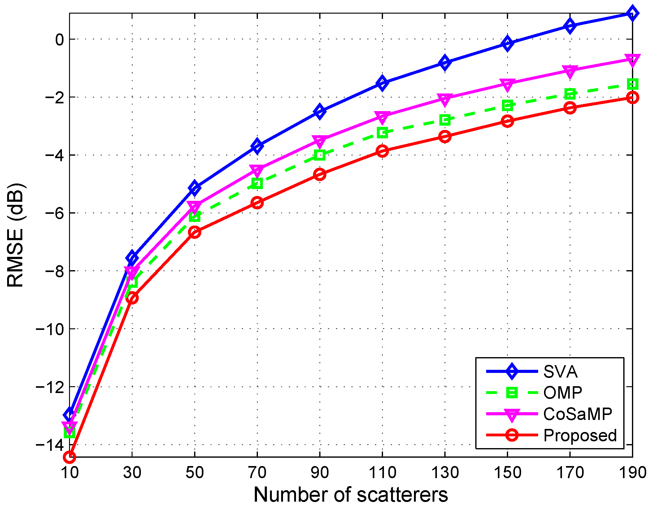
The number of scattering points in the target area will directly affect the imaging quality. In the following experiment, the performance of the proposed method versus different number of scatterers will be investigated. The configuration of this simulation is the same as Section 4.1.1. The SNR is set to 5 dB, and the RMSE curves are shown in Figure 13.
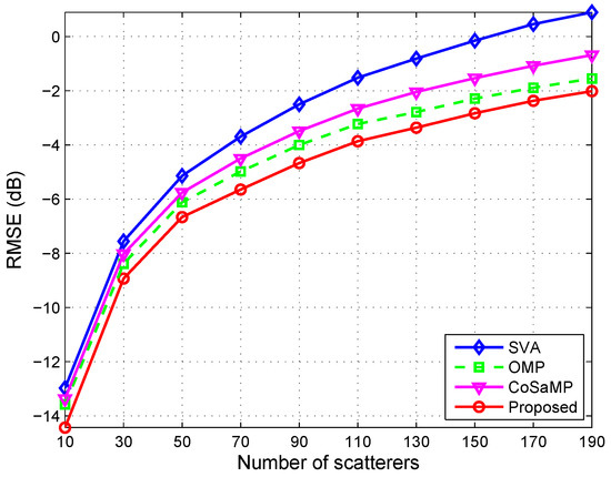
Figure 13.
RMSE comparison versus different number of scatterers (, SNR = 5 dB, ).
The simulation result indicates that the performance of proposed method is superior to the reference methods with all the test scenarios. When the numbers of scatterers is less than 30, the performance of all reference methods seems to be close. With the number of scatterers increasing, the performance of SVA, limited by the resolution of itself, becomes worse. The sparse-reconstruction-based methods with super-resolution maintain better robustness even as the scatterers become dense. Exploiting the structured feature of target, the proposed method provides the advantage for imaging, and achieves effective sidelobe control. Of all the curves of RMSE versus scatterer quantity, the one of the proposed method grows most slowly and always has the lowest RMSE value, according to the curves shown in Figure 13. Even the number of scatterers is larger than 90, the RMSE of the proposed method is still lower 3 dB than that of the SVA method.
4.2.2. Computational Resource Requirement
This group of experiments investigate the requirements for computing resources of different methods. The evaluation indicator is CPU time. The configuration of this experiment is the same as in Section 4.2.1. The statistical results for the case of different SNRs are shown in Table 2.

Table 2.
Average running time of each algorithm versus different SNRs.
The last experiment considers the case of different number of scatter points. Setting the configuration be the same as in Section 4.2.1, the statistical results are shown in Table 3.

Table 3.
Average running time of each algorithm versus different number of scatterers.
From the statistical results in Table 2 and Table 3, it is shown that the fastest algorithm is SVA, the second fastest one is the proposed method, followed by CoSaMP and OMP in sequence. Although SVA is the fastest algorithm, its performance is the worst among all these methods, especially in the low SNR case, which is shown in Figure 12. Compared with this, OMP and CoSaMP perform better, but both the two algorithms require a large amount of system resources. Since OMP algorithm needs to match every atom at each iteration step, it runs extremely time-consuming, which means it unsuitable for the real-time applications. So far as that is concerned, the proposed method of this paper could not only run faster one order of magnitude than CoSaMP, but also ensure the better performance than the latter, which determines its prominent advantages in practical applications.
5. Conclusions
In this paper, a tensor decomposition algorithm for the spotlight SAR imaging is developed based on Tucker model which formulizes SAR echo signal with Kronecker constraint. Under the common scenario in SAR imaging, the scatterers usually cluster together and the targets are sparsely located. This structured sparse feature provides a prerequisite for the proposed method. Not only has this method better robustness for signal reconstruction, but also produces less algorithm complexity and requires smaller computation resource as well, due to exploiting the Kronecker information in each mode sufficiently.
In comparison with the existing SAR imaging methods, such as the SVA and classic matching pursuit algorithms, the proposed method performs much better with respect to robustness about noise and sidelobe disturbance. Numerical analysis has demonstrated that the recovery upper bound of the multiway sparse reconstruction based on structured sparsity is larger than that of the classic matching pursuit methods. Both the theoretical analysis and simulation results also indicate that the proposed algorithm requires much less computational resources than the reference methods, which is by far the most important in practical applications.
Acknowledgments
This work was supported in part by the National Natural Science Foundation of China (NSFC) under Grants (U1533125 and 61401069) and National Science and technology major project under Grant 2016ZX03001022. The authors would like to thank the anonymous reviewers for their valuable comments that significantly improved the quality of this paper.
Author Contributions
Yu-Fei Gao conceived and verified the feasibility of SAR imaging by introducing tensor modeling, and proposed the multiway structured sparse target reconstruction algorithm based on tensor decomposition; Yu-Fei Gao, Xun-Chao Cong and Yue Yang performed the experiments; Qun Wan contributed the design of numerical simulations; Yu-Fei Gao wrote this paper; Xun-Chao Cong, Yue Yang and Guan Gui checked the manuscript and contributed to the rearrangement of the materials. All authors have read and approved the final manuscript.
Conflicts of Interest
The authors declare no conflict of interest.
References
- Curlander, J.C.; McDonough, R.N. Synthetic Aperture Radar: Systems and Signal Processing; Wiley-Interscience: New York, NY, USA, 1991. [Google Scholar]
- Franceschetti, G.; Lanari, R. Synthetic Aperture Radar Processing; CRC Press: Boca Raton, FL, USA, 1999. [Google Scholar]
- Vu, D.H. Advanced Techniques for Synthetic Aperture Radar Image Reconstruction. Ph.D. Thesis, University of Florida, Gainesville, FL, USA, 2012. [Google Scholar]
- Soumekh, M. Synthetic Aperture Radar Signal Processing with MATLAB Algorithms; Wiley-Interscience: New York, NY, USA, 1999. [Google Scholar]
- Donoho, D.L. Compressed sensing. IEEE Trans. Inf. Theory 2006, 52, 1289–1306. [Google Scholar] [CrossRef]
- Eldar, Y.C.; Kutyniok, G. Compressed Sensing: Theory and Applications; Cambridge University Press: Cambridge, UK, 2012. [Google Scholar]
- Liu, Y.; Tao, T. A CS Recovery Algorithm for Model and Time Delay Identification of MISO-FIR Systems. Algorithms 2015, 8, 743–753. [Google Scholar] [CrossRef]
- Çetin, M.; Karl, W.C. Feature-enhanced synthetic aperture radar image formation based on nonquadratic regularization. IEEE Trans. Image Proc. 2001, 10, 623–631. [Google Scholar] [CrossRef] [PubMed]
- Baraniuk, R.; Steeghs, P. Compressive radar imaging. In Proceedings of the 2007 IEEE Radar Conference, Chantilly, VA, USA, 17–20 April 2007; pp. 128–133.
- Gurbuz, A.C.; McClellan, J.H.; Scott, W.R. A compressive sensing data acquisition and imaging method for stepped frequency GPRs. IEEE Trans. Signal Proc. 2009, 57, 2640–2650. [Google Scholar] [CrossRef]
- Potter, L.C.; Ertin, E.; Parker, J.T.; Cetin, M. Sparsity and compressed sensing in radar imaging. Proc. IEEE 2010, 98, 1006–1020. [Google Scholar] [CrossRef]
- Batu, O.; Cetin, M. Parameter selection in sparsity-driven SAR imaging. IEEE Trans. Aerosp. Electron. Syst. 2011, 47, 3040–3050. [Google Scholar] [CrossRef]
- Fang, J.; Xu, Z.; Zhang, B.; Hong, W.; Wu, Y. Fast compressed sensing SAR imaging based on approximated observation. IEEE J. Sel. Top. Appl. Earth Obs. Remote Sens. 2014, 7, 352–363. [Google Scholar] [CrossRef]
- Zhang, X.; Liao, G.; Zhu, S.; Yang, D.; Du, W. Efficient compressed sensing method for moving-target imaging by exploiting the geometry information of the defocused results. IEEE Geosci. Remote Sens. Lett. 2015, 12, 517–521. [Google Scholar] [CrossRef]
- Cong, X.; Gui, G.; Li, X.; Wen, G.; Huang, X.; Wan, Q. Object-level SAR imaging method with canonical scattering characterisation and inter-subdictionary interferences mitigation. IET Radar Sonar Navig. 2016, 10, 784–790. [Google Scholar] [CrossRef]
- Zhao, L.; Wang, L.; Bi, G.; Li, S.; Yang, L.; Zhang, H. Structured sparsity-driven autofocus algorithm for high-resolution radar imagery. Signal Proc. 2016, 125, 376–388. [Google Scholar] [CrossRef]
- Bro, R. PARAFAC. Tutorial and applications. Chemom. Intell. Lab. Syst. 1997, 38, 149–171. [Google Scholar] [CrossRef]
- Sidiropoulos, N.D.; Bro, R.; Giannakis, G.B. Parallel factor analysis in sensor array processing. IEEE Trans. Signal Proc. 2000, 48, 2377–2388. [Google Scholar] [CrossRef]
- Gao, Y.F.; Zou, L.; Wan, Q. A two-dimensional arrival angles estimation for L-shaped array based on tensor decomposition. AEU-Int. J. Electron. Commun. 2015, 69, 736–744. [Google Scholar] [CrossRef]
- Donoho, D.L. High-dimensional data analysis: The curses and blessings of dimensionality. In Proceedings of the AMS American Math Society Challenges Lecture, Los Angeles, CA, USA, 6–11 August 2000; pp. 1–32.
- Oseledets, I.V.; Tyrtyshnikov, E.E. Breaking the curse of dimensionality, or how to use SVD in many dimensions. SIAM J. Sci. Comput. 2009, 31, 3744–3759. [Google Scholar] [CrossRef]
- Cichocki, A.; Mandic, D.; de Lathauwer, L.; Zhou, G.; Zhao, Q.; Caiafa, C.; Phan, H.A. Tensor decompositions for signal processing applications: From two-way to multiway component analysis. IEEE Signal Proc. Mag. 2015, 32, 145–163. [Google Scholar] [CrossRef]
- Lim, L.H.; Comon, P. Multiarray signal processing: Tensor decomposition meets compressed sensing. Comptes Rendus Mec. 2010, 338, 311–320. [Google Scholar] [CrossRef]
- Duarte, M.F.; Eldar, Y.C. Structured Compressed Sensing: From Theory to Applications. IEEE Trans. Signal Process. 2011, 59, 4053–4085. [Google Scholar] [CrossRef]
- Sidiropoulos, N.D.; Kyrillidis, A. Multi-way compressed sensing for sparse low-rank tensors. IEEE Signal Proce. Lett. 2012, 19, 757–760. [Google Scholar] [CrossRef]
- Caiafa, C.F.; Cichocki, A. Computing sparse representations of multidimensional signals using kronecker bases. Neural Comput. 2013, 25, 186–220. [Google Scholar] [CrossRef]
- Caiafa, C.F.; Cichocki, A. Multidimensional compressed sensing and their applications. Wiley Interdiscip. Rev. Data Min. Knowl. Discov. 2013, 3, 355–380. [Google Scholar] [CrossRef]
- Stankwitz, H.C.; Dallaire, R.J.; Fienup, J.R. Nonlinear apodization for sidelobe control in SAR imagery. IEEE Trans. Aerosp. Electron. Syst. 1995, 31, 267–279. [Google Scholar] [CrossRef]
- Walter, G.C.; Ron, S.G.; Ronald, M.M. Spotlight Synthetic Aperture Radar; Artech House Publishers: Norwood, MA, USA, 1995. [Google Scholar]
- Tropp, J.A. Greed is good: Algorithmic results for sparse approximation. IEEE Trans. Inf. Theory 2004, 50, 2231–2242. [Google Scholar] [CrossRef]
- Needell, D.; Tropp, J.A. CoSaMP: Iterative signal recovery from incomplete and inaccurate samples. Appl. Comput. Harmon. Anal. 2009, 26, 301–321. [Google Scholar] [CrossRef]
- Tropp, J.A.; Wright, S.J. Computational methods for sparse solution of linear inverse problems. Proc. IEEE 2010, 98, 948–958. [Google Scholar] [CrossRef]
- Greengard, L.; Lee, J. Accelerating the Nonuniform Fast Fourier Transform. SIAM Rev. 2004, 46, 443–454. [Google Scholar] [CrossRef]
- Jokar, S.; Mehrmann, V. Sparse solutions to underdetermined Kronecker product systems. Linear Algebra Appl. 2009, 431, 2437–2447. [Google Scholar] [CrossRef]
- Duarte, M.F.; Baraniuk, R.G. Kronecker compressive sensing. IEEE Trans. Image Process. 2012, 21, 494–504. [Google Scholar] [CrossRef] [PubMed]
- Caiafa, C.F.; Cichocki, A. Stable, robust, and super fast reconstruction of tensors using multi-way projections. IEEE Trans. Signal Process. 2015, 63, 780–793. [Google Scholar] [CrossRef]
- Kolda, T.G.; Bader, B.W. Tensor decompositions and applications. SIAM Rev. 2009, 51, 455–500. [Google Scholar] [CrossRef]
- Eldar, Y.C.; Mishali, M. Block sparsity and sampling over a union of subspaces. In Proceedings of the 2009 16th International Conference on Digital Signal Processing, Santorini, Greece, 5–7 July 2009; pp. 1–8.
- Eldar, Y.C.; Kuppinger, P.; Bolcskei, H. Block-Sparse Signals: Uncertainty Relations and Efficient Recovery. IEEE Trans. Signal Process. 2010, 58, 3042–3054. [Google Scholar] [CrossRef]
- Rubinstein, R.; Zibulevsky, M.; Elad, M. Efficient Implementation of the K-SVD Algorithm Using Batch Orthogonal Matching Pursuit; Technical Report 8; Computer Science Department, Technology—Israel Institute of Technology: Haifa, Israel, 2008. [Google Scholar]
© 2016 by the authors. Licensee MDPI, Basel, Switzerland. This article is an open access article distributed under the terms and conditions of the Creative Commons Attribution (CC BY) license ( http://creativecommons.org/licenses/by/4.0/).

