1. Introduction
The impact detection and identification strategy for existing structures is of primary importance both in structural health monitoring (SHM) and in non-destructive evaluation (NDE) techniques. Accurately detecting and characterizing an impact event based on sensor data leads us towards condition-based monitoring (CBM), where the subsequent damage can then be detected through active sensing strategies [
1,
2,
3,
4,
5,
6,
7]. Impact identification procedures have been investigated in the last two decades, both numerically and experimentally [
8,
9,
10,
11,
12,
13,
14]. Many of the impact localization methods use the triangulation technique based on the time of flight (ToF) of the waves generated due to an impact and captured by sensors. This approach is limited by the assumption that wave velocity must be known and remain the same in all directions. However, this is not the case for anisotropic and inhomogeneous materials. Moreover, the flexural wave velocity is not constant, and it is a function of the signal frequency, which depends on the impact mass and velocity. Methodologies applicable to anisotropic structures can be grouped into three techniques:
Build meta-models between the sensor response and the impacts by using an inverse analysis. Such an example is the time reversal method [
8]; however, once the response of the structure becomes non-linear (presence of damage), the method is not applicable. To account for the non-linearity of the problem, the genetic algorithm (GA) and artificial neural networks (ANN) have been proposed. In [
9,
10], ANNs were established, using a large dataset of various impact scenarios obtained numerically, to predict impact location and impact force distribution
Having a distributed sensor array in the structure and using the hyperbolic positioning algorithm. In [
11], Ciampa et al. proposed a strategy to locate impact in composite plates with six piezoelectric (PZT) sensors by calculating the time difference between each sensor. However, this techniques require an accurate estimate of the wave velocity, which is only achieved by placing the sensors in optimized locations. This might be an issue for built-up structures
Sensor rosettes are used to estimate the wave propagation direction. In [
14], Zhang et al. has used a metal-core piezoelectric fibre (MPF) sensor rosette to detect and localize impacts on metallic plates. A new procedure proposed by Zamorano et al. [
13] uses groups of closely-spaced embedded sensors to calculate the angle of the impact. The method was validated for high velocity impact where the impactor pierces the composite panel. In a recent study, Qiu et al. [
15] have adopted a spatial-wavenumber filtering technique with a dense 2D cross-shaped linear array of piezoelectric sensors to detect the impact direction and the distance relative to the sensor array. The validation results on composite structures show that the impact direction can be estimated accurately, but the accuracy of the impact location estimation is limited by the error in the group velocity
A key parameter in the reliability of any impact detection algorithm is the optimal number and location of sensors (see the review in [
16]). Most of the impact detection and identification research is carried out in a controlled laboratory environment. However, in real structures under operational conditions, there will be many factors influencing the recorded signals. In general, uncertainties can be caused by random and systematic errors, and it is important to consider them in the design and optimisation of any SHM system for the application to real structures. The basic idea of the Bayesian approach is to treat some variables, denoted by the vector
θ, as random variables with joint distribution
. It aims at calculating the posterior (updated) distributions of uncertain parameters for a given set of measured data. Such an approach has been often adopted in SHM techniques in the damage identification framework [
17,
18].
A probabilistic framework for acoustic emission (AE) source localization with PZT sensors in plate-like structures is developed in [
19] and validated on an aluminium plate. The ToF and the wave velocity are considered as mutually-independent Gaussian random variables. The continuous wavelet transform (CWT) is applied to the ToF measurements, and the resulting variances in time domain and in frequency domain are correlated to the uncertainty in arrival time and in group velocity, respectively, by invoking the Heisenberg uncertainty. The extended kalman filter (EKF) is used to estimate the AE source location and the wave velocity provided that the ToF measurements and the previous variances are given.
An early contribution to the optimal sensor placement problem for damage detection laying out a theoretical framework rooted in Bayes risk is provided in [
20]. The general form of the Bayes risk is first investigated and then minimized in order to provide the optimal detector, i.e., the sensor placement that either maximizes the probability of detection (PoD) or minimizes the false alarm rate. In [
21], Vanli et al. proposed an optimal sensor placement strategy for damage detection to account for the non-uniform likelihood of damages on the structure.
The Bayesian-based optimisation approaches have been developed for active sensing. However, there is little to no evidence of their application to passive sensing. There still remains a challenge for applying the developed methodologies and algorithms to real structures. For example, taking the Airbus A320 family, each zone of the aircraft has a different global percentage of impact, which should be considered when optimizing the sensor locations for a real structure; see
Table 1. Another challenge is to include sensor failures in the reliability analysis of the SHM system.
The main goal of the present paper is to propose a Bayesian-based sensor optimisation strategy aimed at impact identification under varying operational conditions, such as variabilities in the sensor data, sensor failure and the non-uniform probability of impact occurrence. To the authors’ best knowledge, this is the first contribution that encompasses all of the above uncertainties. The passive sensing procedure is based on a meta-modelling technique developed from a large library of impact scenarios on a composite stiffened panel as presented in [
23].
The layout of the paper is as follows: The application of the Bayesian approach to the optimisation framework is detailed in
Section 2 by investigating different sources of uncertainties. The impact detection algorithm is outlined in
Section 2.1 along with details on the adopted artificial neural network strategy. A novel procedure is introduced and implemented in
Section 2.2 in order to include the sensor malfunctioning in the impact identification algorithm. The optimisation process is carried out both excluding and including the probability of sensor malfunctioning, in
Section 2.3 and
Section 2.4, respectively. The computation of the probability of detection, which is necessary to define the objective function of the optimisation process, is detailed in
Section 2.5 by improving the procedure outlined in [
23]. The fitness function and the uncertainty inclusion are validated by experimental and numerical examples in
Section 3 to assess the efficiency and robustness of the proposed procedure. Finally,
Section 4 presents the application of sensor location optimisation on a composite stiffened panel.
2. A Bayesian Sensor Optimisation Algorithm
Here, a Bayesian framework that optimises the sensors’ position in order to maximize the probability of detection of an impact event in the presence of the probability of sensor malfunctioning and variations in the recorded data is described. Two main uncertainties are considered: (i) the error due to factors, such as instrumentation noise, bonding quality, temperature changes, loading and numerical simulation, which may affect the sensor data; (ii) the possible malfunctioning of one or more sensors, which may have failed (damaged or debonded).
The proposed procedure assumes a plate-like structure instrumented with a permanent network of transducers for recording elastic waves generated by an impact event. Each transducer works as a sensor, and it can provide the time of arrival (ToA) of the wave for a given impact. From the knowledge of the ToA from a network of sensors, it is possible to estimate the location of the impact (see
Section 2.1 for a brief overview of the passive sensing methodology).
In order to compute the optimal sensor combination for a given number of sensors, a minimization process needs to be carried out. The optimisation problem is solved by the application of the genetic algorithm as developed in [
23]. The procedure is implemented in the MATLAB program. Individual integer representation, scores and selection, crossover and mutation are taken from [
23]. The main improvements of the code are related to the computation of the fitness function, i.e., functions
and
, which will be thoroughly described in this section.
2.1. Impact Detection Algorithm
The passive sensing algorithm used in this work for impact detection is based on the ANN technique developed in [
9,
23] to detect the location of an impact from sensor readings. ANN is a machine learning algorithm that uses a set of training data to build a non-linear function relating a set of input data to output data. It adapts its structure (weights) based on the input and output of the system during the learning phase. The input, in this case, is sensor signals recorded during an impact event, and the output is given by the
x and
y coordinates of the impact location. To reach a regularization, the ANN needs to be trained with a wide range of data, i.e., impact scenarios representing probable impact cases for the structure under analysis. It is unrealistic to assume that all of the required data can be obtained experimentally due to the large number of possible impacts. Therefore, in this work, a vast library of impact scenarios (different locations and energies), which are likely to occur during the life-time of an aircraft fuselage, were obtained by performing impact simulations on a composite stiffened panel using a validated non-linear Finite Element (FE) model. The impacts cover all of the possible locations, i.e., mid-bay, under/over the stringer and on the foot of the stringer. In addition, different types of impacts (large mass and small mass) are considered from both inside and outside of the panel. Details of the numerical model and the development of meta models can be found in [
9]. The recorded sensor signals, in their discrete form, should not be used as inputs to the ANN because they contain too much information. When there are too many input parameters in the model compared to the number of training patterns, there will be the problem of overfitting, and the meta-model will not reach a converged solution. Therefore, feature extraction is applied to the sensor data. The feature used in this work as input to the ANN is the ToA of each sensor signal. The features extracted from each signal are weighted and passed into the input layer, which is connected to the hidden layer and the output layer through the non-linear activation function. The novelty of the current work is the inclusion of uncertainties in the input data (ToA) in a statistical framework and the addition of the probability of sensor malfunctioning in the ANN generation. It must be pointed out that the proposed optimisation approach is independent of the impact identification algorithm. It can be implemented with any impact identification procedure, using either experimental or numerical data.
2.2. Inclusion of Sensor Malfunctioning into Impact Detection
In this section, a procedure to include the malfunctioning sensor in the impact identification algorithm is presented. The way its probability of occurrence is included in the optimisation process will be discussed in the
Section 2.4.
The monitored structures are usually subjected to various external load and environmental conditions that may adversely affect the functionality of the SHM sensors. Impacts may also be responsible for sensor failures. Because piezoceramic materials are brittle, sensor fracture and subsequent degradation of mechanical/electrical properties are the most common types of sensor failures. In addition, the integrity of the bonding between a PZT sensor and a host structure should be maintained and monitored throughout its service life. A completely broken sensor (hard fault) can be identified when the sensor does not produce any measurable output. However, if the sensor or the bonding is partially damaged or deteriorated, the distorted signal can potentially lead to a false indication of impact (soft fault).
There are established techniques to determine faulty sensors prior to any acquisition; see, for instance [
24,
25,
26,
27,
28]. The degradation of the PZT sensor may also be detected by measuring the change in the imaginary part of the electrical admittance [
7,
29]. In this work, the probability that one or more sensors may be malfunctioning during the structural monitoring is included in the optimisation process. Sensor fault malfunctioning (either soft or hard) is included in the optimisation procedure by removing the ToA of the faulty sensor from the analysis. The reasoning for this approach is to increase the reliability of the detection by having more than one trained ANN for any given sensor combination.
The optimisation can be carried out using either experimental data, or numerical data, or a combination of both. The iterative sensor combination can be tested by building its representative ANN together with all of the possible ANNs obtained from the pristine sensors by removing
sensors, where
provides the pre-defined number of possible faulty sensors. In such an alternative, a known number of ANNs needs to be generated for each sensor combination involved in the optimisation process. If
is a matrix including all of the possible sensor combinations generated from the original one by removing the faulty sensors, the procedure can be written as:
The faulty sensors are selected following the probability distribution
. Two different sub-options have been considered here. In the former (Option A), exactly
faulty sensors are envisaged. This means that
ANNs need to be built for each sensor combination to be tested in the optimisation process:
In the latter (Option B),
indicates the maximum number of probable faulty sensors, i.e., the ANNs to be generated are all of the ANNs extracted from the sensor combination under analysis by removing all of the
k faulty sensors with
k going from one to
:
2.3. Inclusion of the Uncertainty in the ToA
The measurement uncertainties are described by two variables and , respectively. The former is related to the error introduced by variation in material properties and geometrical tolerances (either numerical or experimental) that may influence the ToA measurement, while the latter is related to the noise introduced by the instrumentation (cross-talk, background noise) and/or environmental conditions (temperature, humidity). It is worth pointing out that the proposed approach is valid for data collected experimentally or simulated numerically. What is included here is the influence of the variability of the measured data on the optimisation process, regardless of how they are generated.
The probabilistic description of the measured ToA in the
i-th sensor can be expressed as:
where
and
are the measured and computed ToA in the
k-th sensor, respectively. The computed ToA is obtained from the signals simulated by the FE analysis. For simplicity and without loss of generality,
and
are assumed to be two independent Gaussian variables with zero mean and standard deviation
and
, respectively. If the ToA
(
being the total number of sensors) are assumed to be independent and identically distributed, the likelihood for any
k can be expressed as:
where
gives the position of the impact,
μ the mean of the distribution and
means the total variance. The above probabilistic approach is included in the optimisation procedure. The mean value can be assumed to be equal to the computed ToA.
Using Bayes’ theorem, the likelihood can be related to the posterior probability distribution function (PDF) and to the prior distribution as:
The above relation may be used to determine the location of the impact on the basis of the sensors measurements (for instance, to locate the damage in [
17,
30]). However, in this work, the Bayes theory is used for sensor optimisation, while the impact detection, as explained in
Section 2.1, is performed by an ANN approach.
The optimal sensor configuration can be obtained by solving the following problem:
where
is a vector collecting the sensor readings,
I is a set of given impacts each of which is located at
,
and represents the Euclidean distance between the actual impact location and the predicted impact location. The vector
represents a threshold value representing the acceptable performance of the SHM system to detect the impact, and for the sake of generality, it can be assumed to be a function of the impact position.
The minimization given in Equation (
5) means that the optimal sensor configuration is searched in order to minimize the probability of not detecting an impact occurring at location
. As the impact events are independent, the above problem can be stated as:
where
C is a constant to scale the probability function in the range
, and it can be set equal to the number of impacts in
I. By applying Bayes’ theorem, we obtain:
where
is the probability that the impact occurring in
is identified with an error
. The relation (
7) is equivalent to the minimization of the Bayes risk as presented in [
20] with reference to the damage identification.
If the ToA measurements are assumed to obey Equation (
3), then
is the conditioned marginal probability of
, i.e.,:
The prior probabilities
and
can be stated as the mathematical representation of the engineering judgement on the unknown variables (the impact location and the variance of the measurement) with the purpose of including any available knowledge prior to the application of the monitoring system in real operation [
31]. For composite panels in aeronautics, such terms can be built, for instance, by gathering the impact monitoring data from the fleet.
The integral in Equation (
8) can be computed numerically by imposing
to vary in a fixed pre-defined interval. The
term can be computed by following a Monte Carlo approach and varying the ToA in each sensor in the Gaussian representation. More details are given in
Section 2.5.
2.4. Sensor Malfunctioning in Optimisation
The Bayesian approach allows a stronger inference between the probability that the impact is identified with the probability that one or more sensors are malfunctioning at the instant of the impact. In this section, a Bayesian sensor optimisation procedure including the probability of sensor failure is presented. The optimal sensor combination can be searched by minimizing the probability of an impact located at
not being detected (i.e.,
) for a given probability of malfunctioning sensors:
where
is a vector identifying the chosen sensor network from the set
containing all of the possible combinations of
, and
is a variable giving the number of malfunctioning sensors. The optimal sensor combination can be searched among a chosen set
I of impacts:
As the impacts are all independent events, it can be written:
where
C is a constant that normalizes the probability sum, and it can be set equal to the number of impacts in
I without loss of generality. By applying Bayes’ theorem and assuming that the impact and the sensor malfunctioning are independent events, we have:
and therefore:
Analogously to what has been proposed in the previous subsection, the marginal probability involved in Equation (
13) can be expressed as:
If
(
) indicates the probability to detect an impact at
for a given sensor malfunctioning level
and a given probability distribution of the ToA measurements, then the minimization process assumes the following expression:
The terms and represent the prior probabilities of having an impact at location , having a level of sensor malfunctioning and having a certain variance in the ToA distribution, respectively. They are the novelty introduced in this work, by the Bayesian approach to improve the optimisation process by taking into account the experience gathered during the service life of the monitoring system.
Notice that the objective function is scalar for a given sensor combination, provided that
has a pre-assigned spatial distribution in terms of the impact position. Details on the computation of the
term are given in
Section 2.5.
2.5. Computation of the Probability of Detection
The evaluation of the probability of detection (PoD), is an important factor in the optimisation analysis, since it represents the performance of the impact detection methodology. In order to optimise the sensor locations for detecting each impact scenario with high reliability, the PoD resulting from different sensor combinations must be maximized through an optimisation approach. The procedure outlined in [
23] for evaluating the PoD is adopted here with several improvements. An iteration of the optimisation process includes developing an ANN for any sensor combination. To evaluate the performance of each ANN, its response is simulated following the Monte Carlo approach with a certain number of samples. Such samples are reproduced by inclusion of the uncertainty in the ToA and sensor malfunctioning
and by considering one impact at a time. The error associated with each sample is given by:
which is the Euclidean distance between the predicted location and the actual location of each impact
i belonging to the test set (all of the available impact scenarios are divided into training, validation and test sets for the development of ANN).
To know which statistical properties best represent the ANN performance, the cumulative distribution function (CDF) must be known. For this reason, the CDF can be built and compared to some analytical distributions. In particular, three analytical CDFs are conceived of by integrating the following three analytical PDFs (a misprint is worth underlining in Equation (
15) of [
23] in the expression of the Weibull PDF):
where
μ and
σ are the mean and standard deviation of the Gaussian PDF;
and
are the mean and the standard deviation of
;
k and
λ are the shape parameter and the scale parameter of the Weibull PDF. A parametric study carried out by the authors concluded that the CDF of the error in Equation (
16) can be described by any of the above functions. In fact, the quantile–quantile plot shows a discrepancy of a maximum of
between the analytical and the numerical CDF.
The analytical function that best describes the probability of detection is identified on the basis of two goodness-of-fit parameters, the normalized root mean square
R and the coefficient of determination
d:
After identifying the best CDF, the probability of detection (either
or
) is computed by reading the
y-value corresponding to
. The present approach stems from [
23] to include statistical analysis of the data: the error is investigated by measuring the influence of the uncertainties on the impact location prediction for each impact, whereas in [
23], the error is only related to the ANN predictions.
4. Optimal Sensor Location for a Composite Stiffened Panel
In the previous section, two examples were presented that validated the proposed fitness function, including uncertainty in the input data (simulating real application) and also accounting for the probability of sensor malfunctioning in the optimisation algorithm. The results concluded that when the sensor malfunctioning is included in the optimisation strategy, the performance of the optimal sensor network is indeed higher than the other sub-optimal combinations.
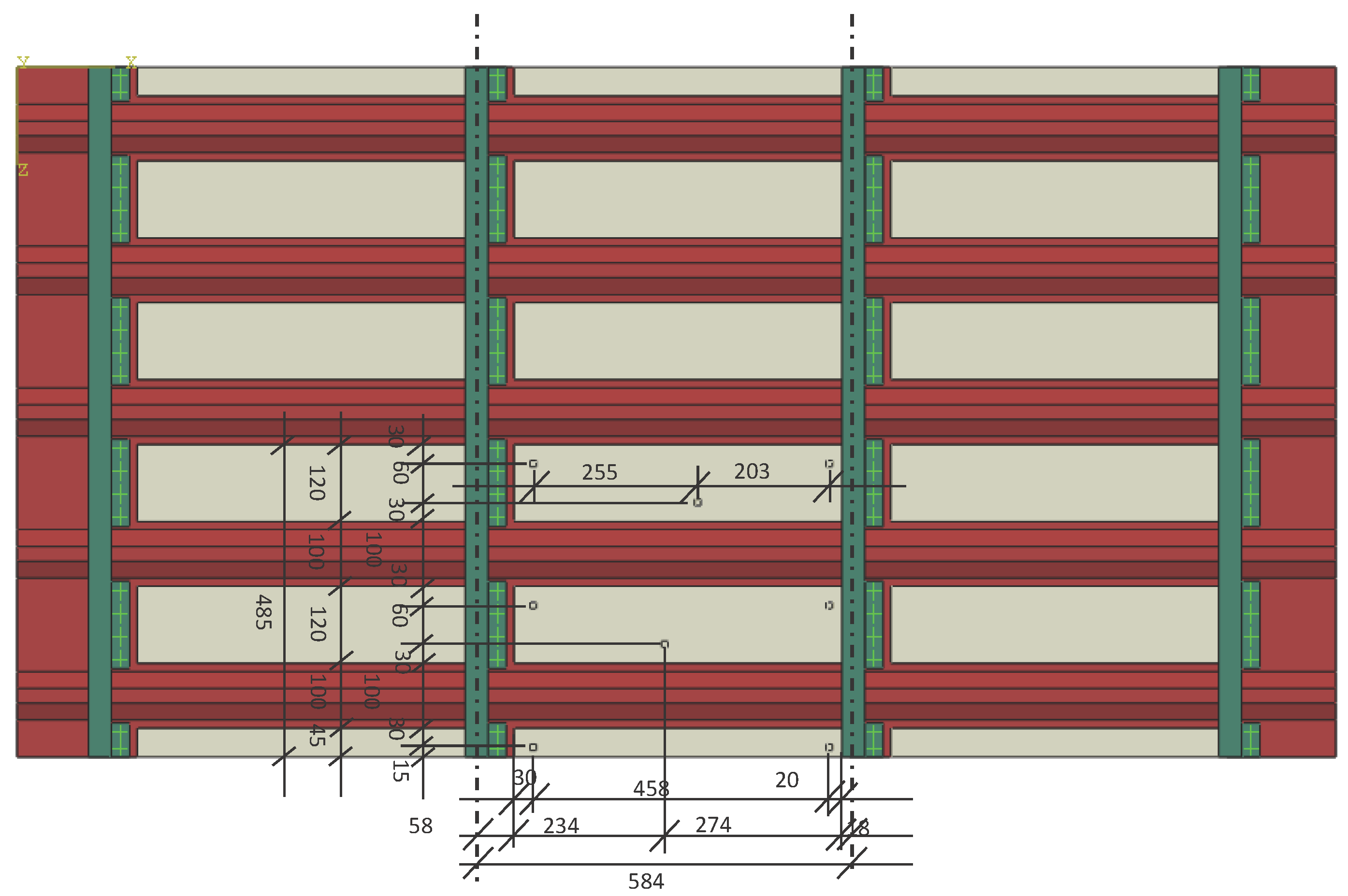
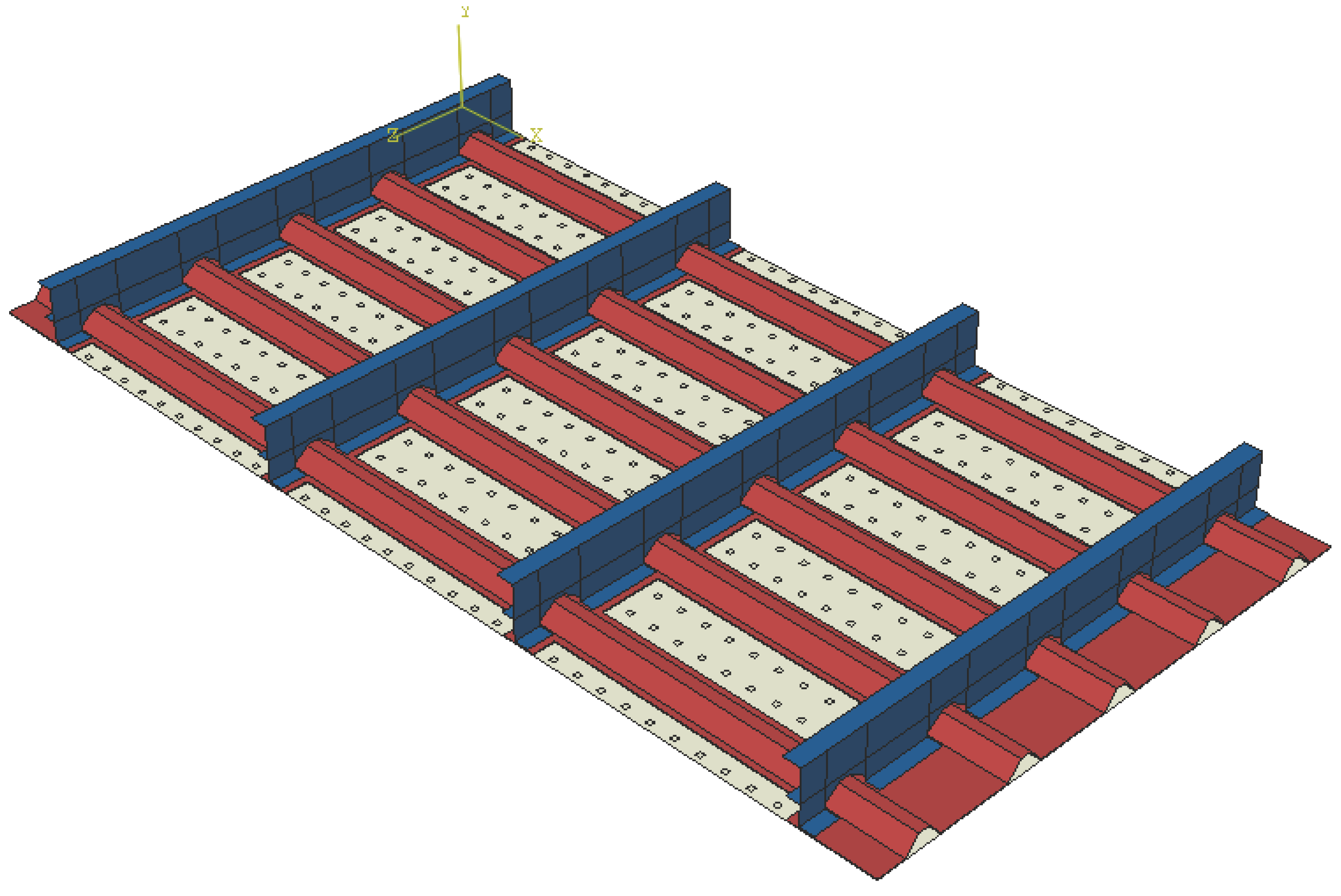
The next step is to assess and validate the proposed strategy by applying it to the full composite stiffened panel depicted in
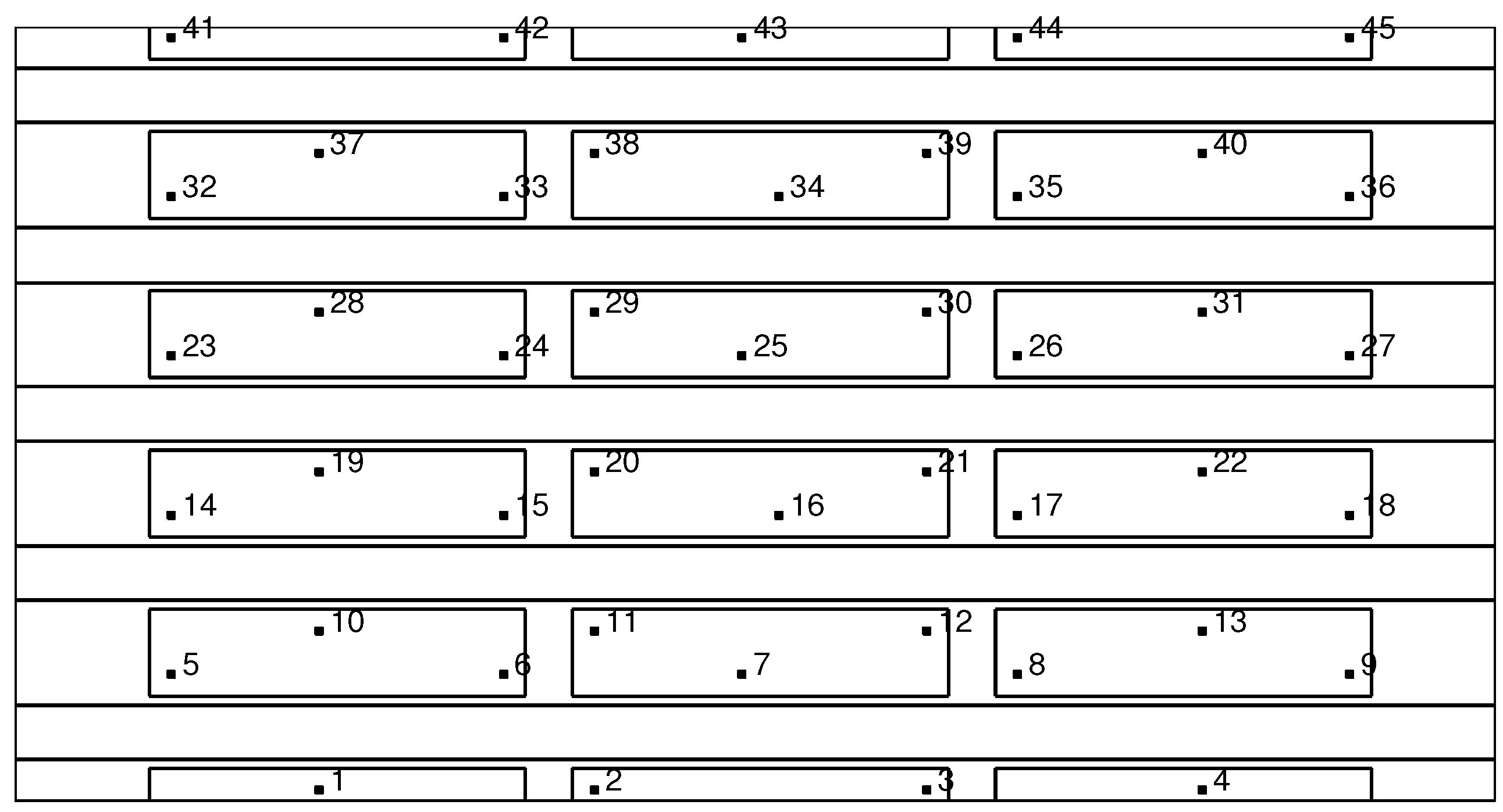
Figure 3. To do so, an optimisation approach based on GA was carried out to find the best four- and five-sensor networks. To reduce the dimensionality and computational cost of the problem, a total of forty-five possible sensor locations has been identified for this example; see
Figure 7.
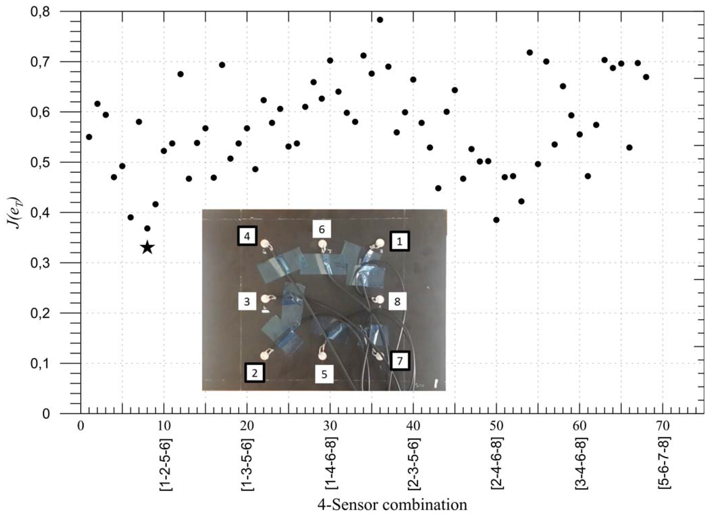
First, the optimisation is carried out to find the best four-sensor combination, with the following parameters: , , , , mm. An initial population of individuals is set. At each iteration of the (GA), a new population of N individuals is generated from the previous one by retrieving elite individuals, mutating with probability and by cross-over of of the parents (where 80 is the percentage out of ). Furthermore, without loss of generality, and are set as uniform distributions.
The optimal sensor combination and its performance are listed in
Table 3. It can be seen that the best performance is achieved when the sensors are placed at the corners of the plate [1-4-41-45], maximizing the coverage area. To validate that the chosen sensor combination is indeed the optimal one, its performance has been compared to similar sensor combinations with similar coverage areas. The results in
Table 3 show that the performances of the sensor networks are very similar, but the optimal one is slightly higher. Furthermore, as expected, their performance deteriorates quickly with increasing the probability of malfunctioning sensors.
So far, in the examples presented, the probability of impact occurrence (i.e.,
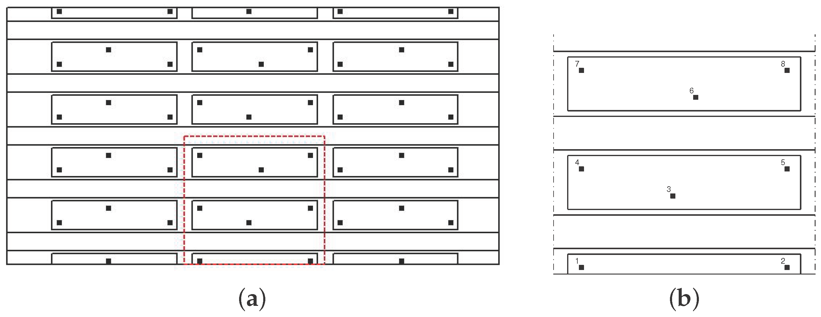
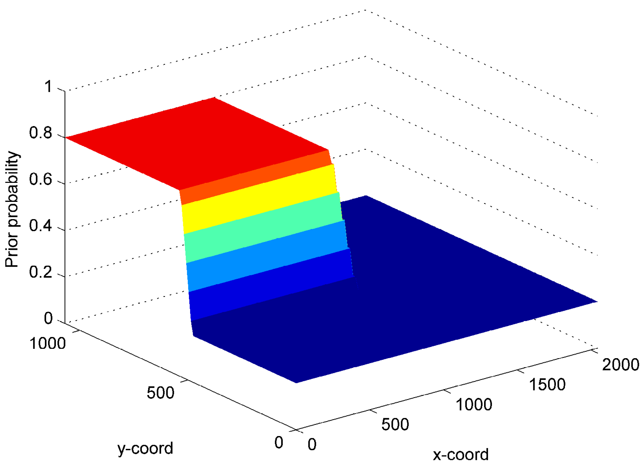
) on the structure is assumed to be uniform. However, a real structure, such as aircraft panels, does not have the same probability of impact occurrence everywhere. One of the advantages of the proposed Bayesian approach is that it allows the user to include a non-uniform probability distribution of impact in the optimisation approach. This feature is presented on the stiffened panel by comparing the best four-sensor combinations with uniform and non-uniform probability distributions
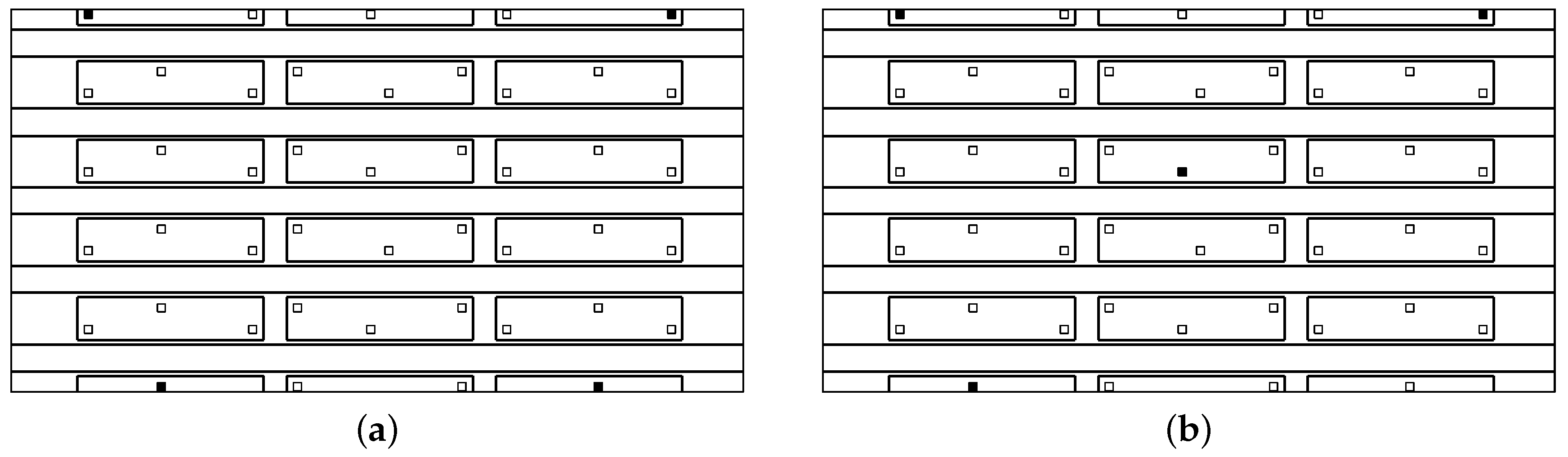
. The non-uniform probability is defined by assuming that it is more likely to have impacts near the top-left corner zone (in an area equal to the half of the entire panel), as presented in
Figure 8. The optimal solutions are depicted in
Figure 9.
For the uniform distribution of
, the minimization process locates the sensors close to the corners (see
Figure 9a). On the contrary, the optimal solution with the non-uniform prior probability has one sensor closer to the area with higher probability of impact (see
Figure 9b). The other three sensors remain in the corner position as the lower probability is set equal to
. Decreasing such a probability would move the three corner sensors towards the top-left area. The performances of the two (uniform and non-uniform) optimal combinations provided in
Figure 9 are listed in
Table 4 (for
,
,
mm).
The last example searches the optimal locations for a five-sensor network, from all of the possible locations in the panel, as shown in
Figure 7. The optimisation procedure is carried out with reference to a detection level of
mm, a Gaussian distribution of ToA provided by
and uniform probability
. All of the remaining parameters are identical to the previous example.
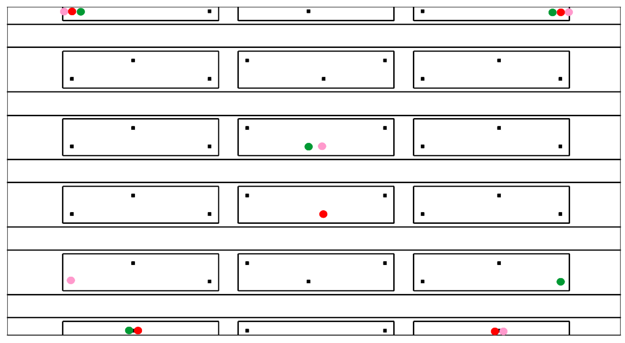
The optimal and sub-optimal combinations are provided in
Figure 10, where they are characterized by different colours, that is red (optimal), green and pink (sub-optimal). The value of
provided by the optimal combination is
. The performance can be improved by reducing the error threshold
; for instance, with
mm, the performance increases to
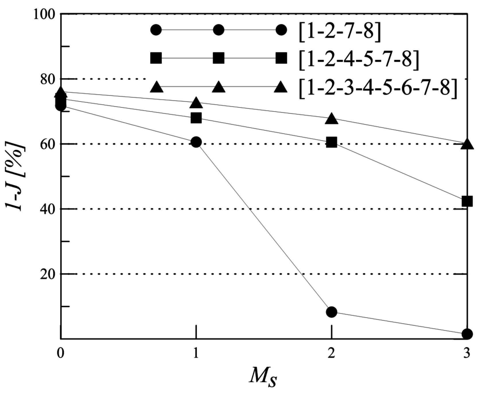
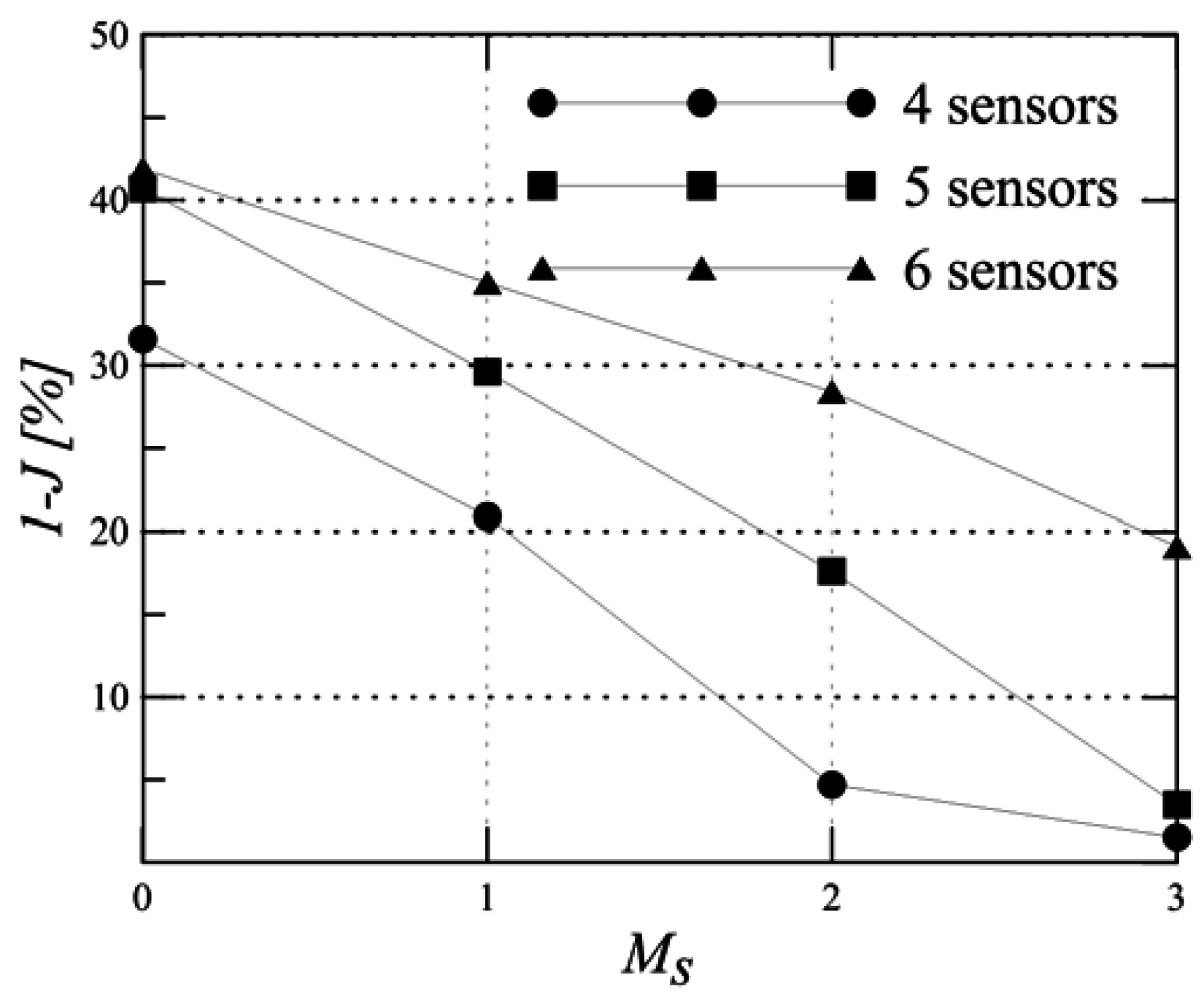
. The comparison between combinations with different numbers of sensors (see
Figure 11) shows that the performance versus the number of sensor malfunctioning
deteriorates more quickly with a lower number of sensors.


