2. Experimental
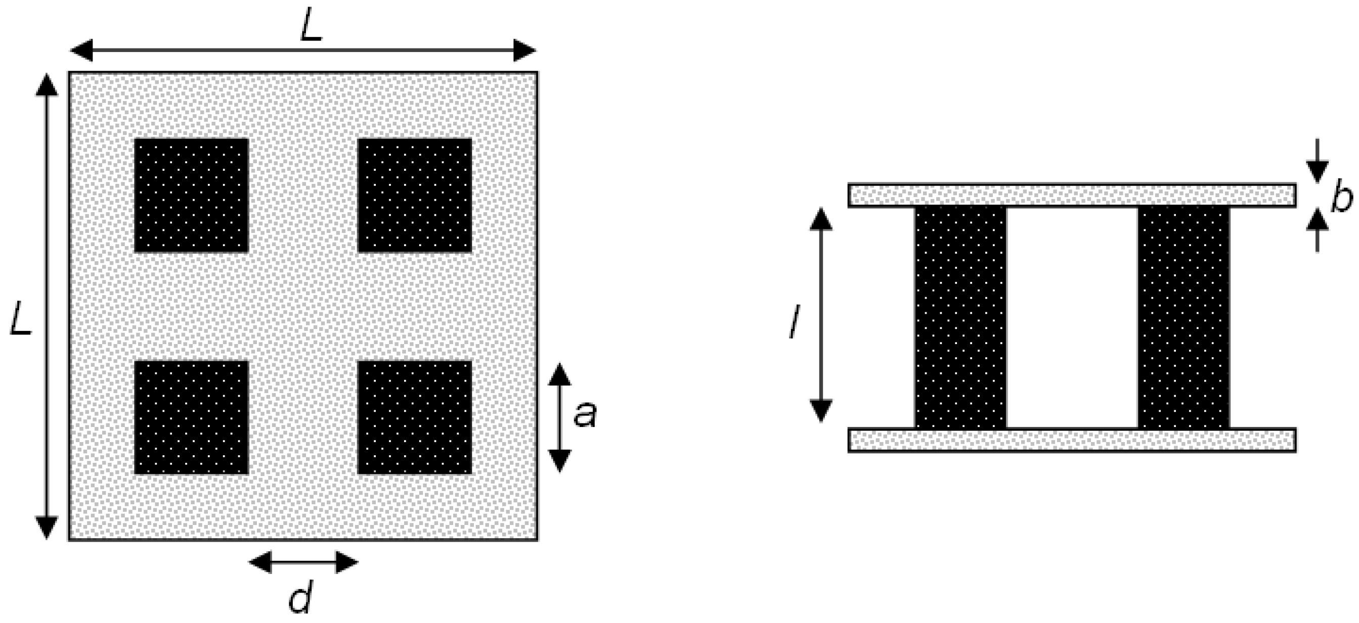
Figure 1 depicts a schematic of a 4-leg TEC module used in the experimental runs. Six demonstrator modules were fabricated with leg lengths
l = 4, 5, and 10 mm (2 modules for each leg length). Each leg has a quadratic cross section of width
a = 4.5 mm and a distance
d = 10 mm from the neighboring leg. The
p-type legs are made of La
1.98Sr
0.02CuO
4; the
n-type legs are made of CaMn
0.98Nb
0.02O
3. These perovskite materials exhibit chemical and mechanical stability at high temperatures, but at the expense of having ZT ~ 0.05 [
13]. The
Lx
Lx
b = 30 × 30 × 0.25 mm absorber (hot) and cooling (cold) plates are made of Al
2O
3 with ~5% porosity. Additionally, the absorber plate is coated with graphite to augment its absorptivity.
Figure 1.
Top and front view of TEC module.
Figure 1.
Top and front view of TEC module.
Experimentation was carried out at the ETH’s High Flux Solar Simulator (HFSS): a high-pressure Ar arc close-coupled to an elliptical reflector that delivers an external source of intense thermal radiation to simulate the heat transfer characteristics of highly concentrating solar systems [
14]. The solar flux concentration is characterized by the mean concentration ratio
, defined as
, where
Qsolar is the solar power intercepted by a target of area
A. The ratio
is often expressed in units of “suns” when normalized to
I = 1 kW/m
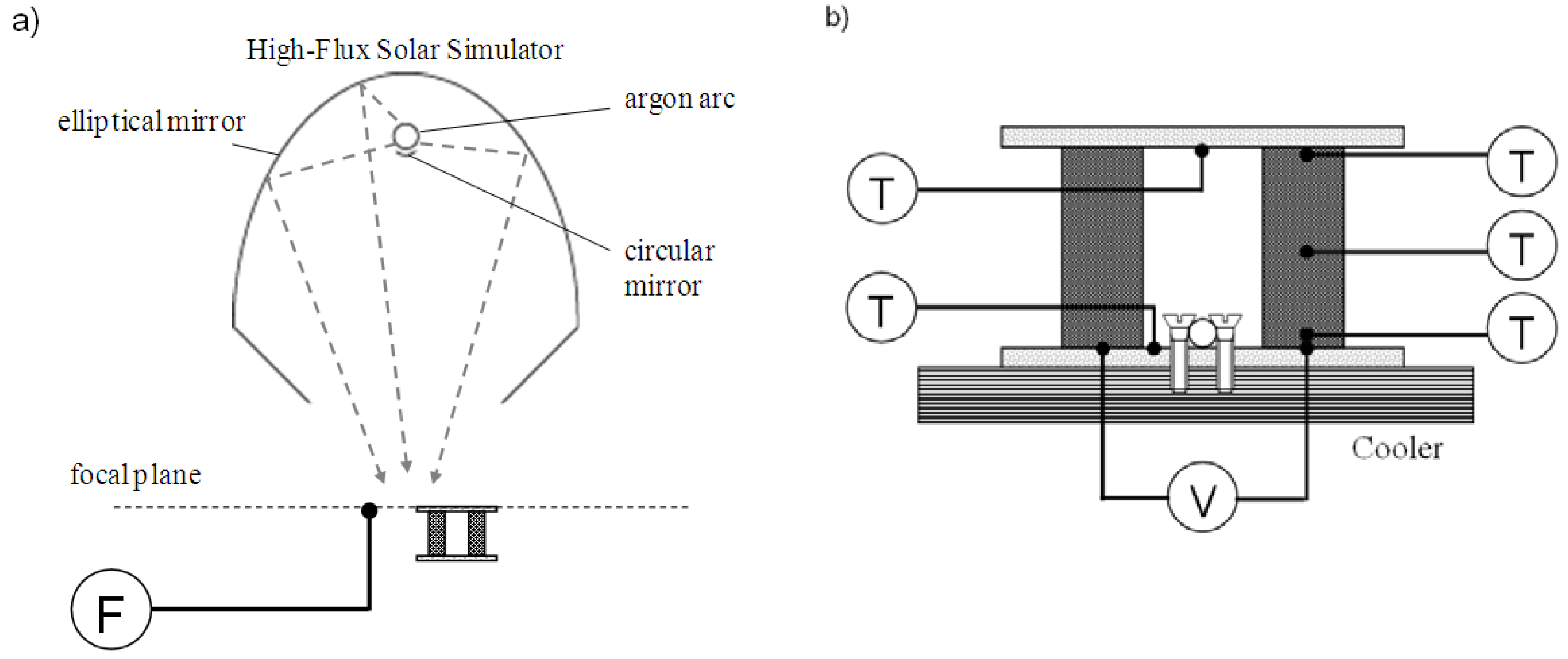
2. The experimental set-up is shown schematically in
Figures 2 (a) and (b). Incident radiative fluxes were measured by a thermogage (with an accuracy of ±3%) [
15], placed symmetrically to the TEC module at the focal plane. The TEC was exposed to a maximum mean solar concentration ratio of 300 suns. K-type thermocouples (tip = 0.5 mm, spatial accuracy = ±0.25 mm) were used to measure temperatures of the plates and of the hot end, middle, and cold end of the legs. Terminals were provided at the cold ends for measuring the voltage/power output of the module. The cold plate was attached to a water-circuit cooler at room temperature.
Figure 2.
Schematic of the experimental setup at ETH’s High Flux Solar Simulator. (a) the TEC module is placed at HFSS’s focal plane; incident solar radiative fluxes measured by a thermogage (F). (b) position of type-K thermocouples (T) used to measure temperatures of the plates and of the hot end, middle, and cold end of the legs; terminals (V) provided at the cold ends for measuring the voltage/power output of the module. The cold plate was attached to a water-circuit cooler (denoted by screw fixation).
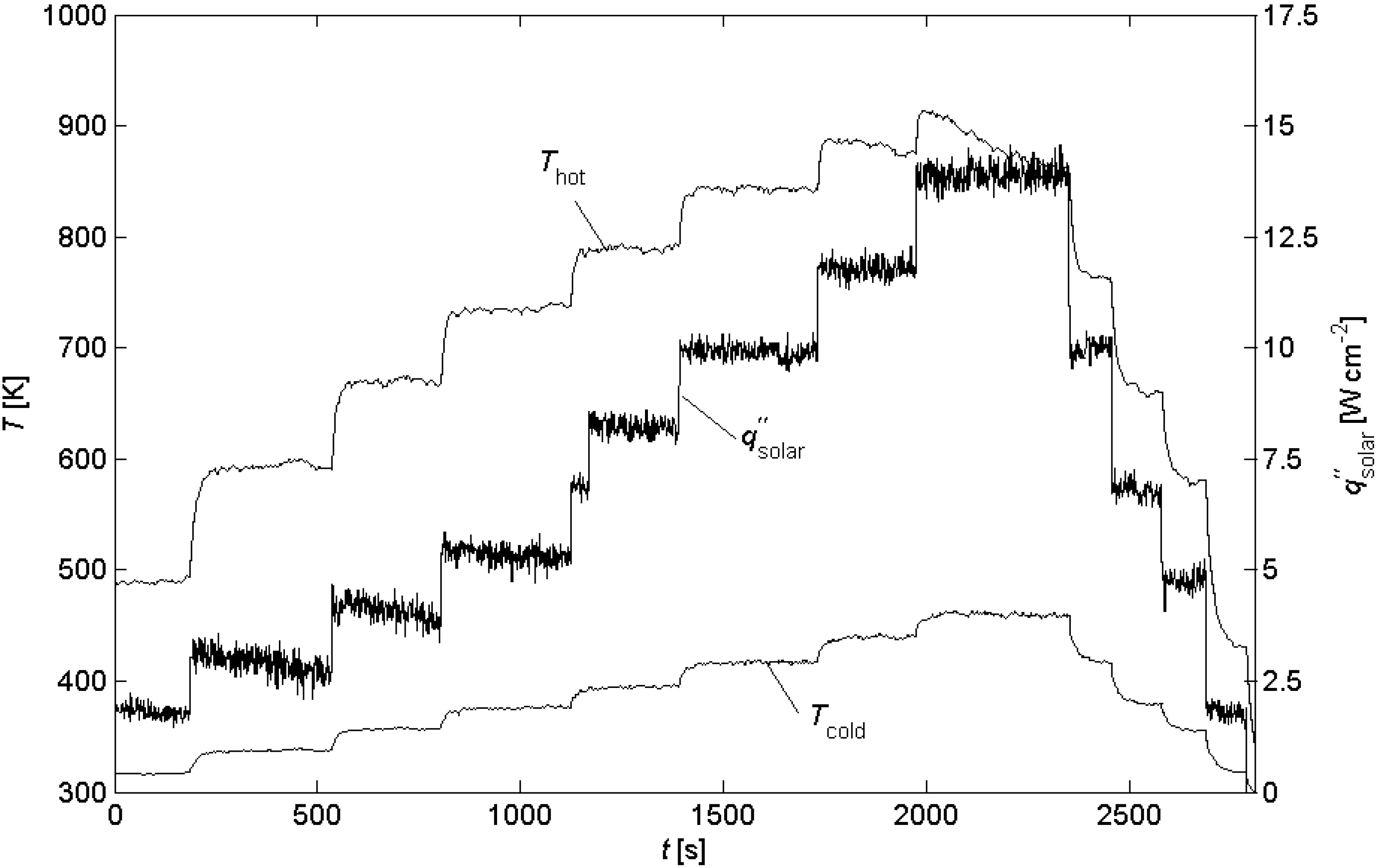
The temperature and solar radiative flux as a function of time are shown in
Figure 3 for a representative experimental run using a module with leg length
l = 4 mm. The incident solar radiation was increased stepwise and held at constant level for 3-5-minute intervals. Due to the low thermal inertia and fast temperature response, steady-state conditions are assumed for each time interval. Maximum temperature was 625°C, at which graphite is no longer stable and starts to burn. For the same module (
l = 4 mm),
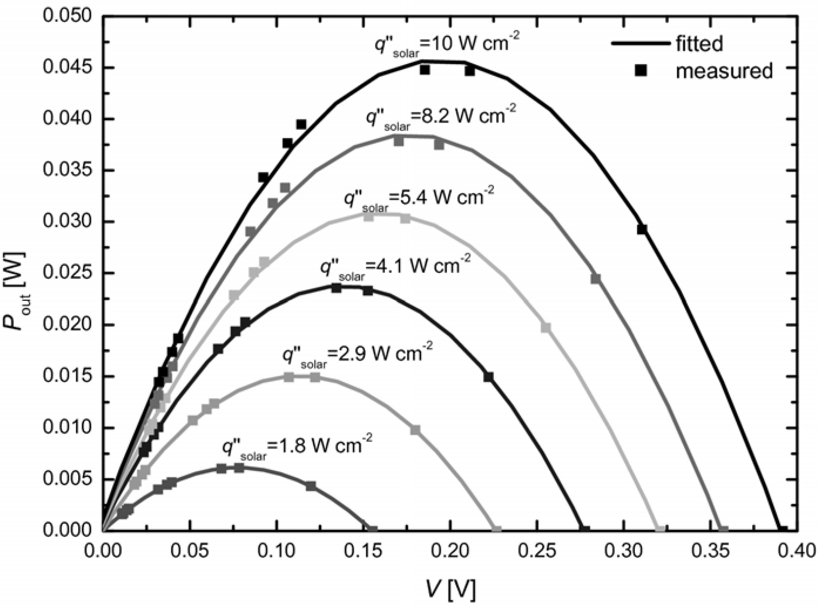
Figure 4 shows the theoretical and measured voltage-power curves for incident solar radiative fluxes in the range
= 1.8–10 W cm
-2, and for external loads with resistance in the range
Rload = 0.1-3.5 Ω. A parabola, which corresponds to the ideal voltage source with an internal resistance [
16], is fitted through the data points. The maximum power is
Pmax = 0.006, 0.015, 0.023, 0.031, 0.038 and 0.046 W for
= 1.8, 2.9, 4.1, 5.4, 8.2 and 10 W cm
-2, respectively.
Figure 3.
Temperature of hot and cold plates and solar radiative flux as a function of time during a representative experimental run for module with l = 4 mm.
Figure 3.
Temperature of hot and cold plates and solar radiative flux as a function of time during a representative experimental run for module with l = 4 mm.
Figure 4.
Fitted and measured voltage-power curves for incident solar radiative fluxes in the range = 1.8 – 10 W cm-2, and for external loads with resistance in the range Rload = 0.1-3.5 Ω for module with l = 4 mm.
Figure 4.
Fitted and measured voltage-power curves for incident solar radiative fluxes in the range = 1.8 – 10 W cm-2, and for external loads with resistance in the range Rload = 0.1-3.5 Ω for module with l = 4 mm.
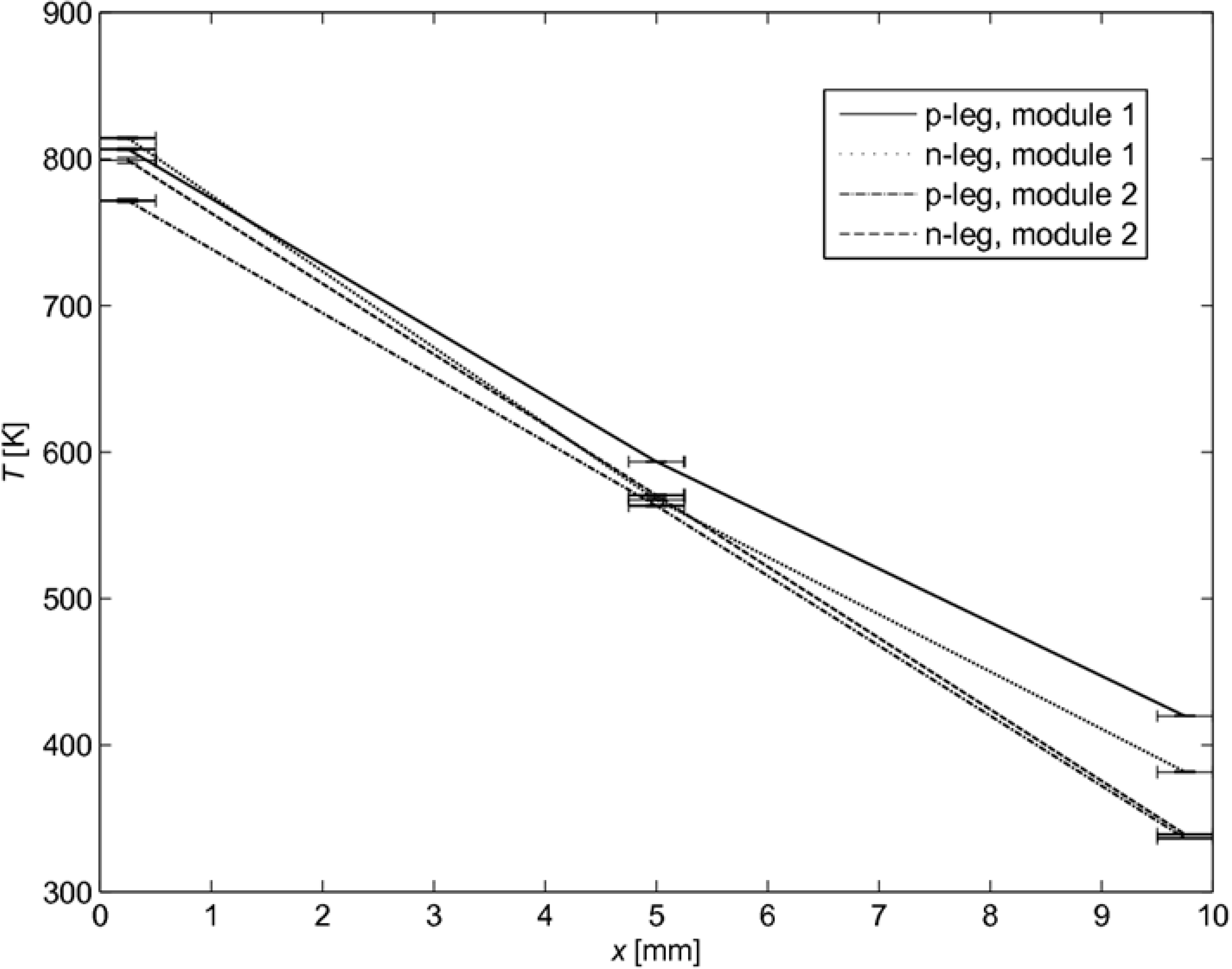
The measured temperature distribution for two tested modules with leg length
l = 10 mm is shown in
Figure 5 for
= 6 W cm
-2. As expected, the quasi linear profile indicates a predominant heat transfer by conduction across the legs. The abnormal behavior of 100 K temperature difference at the cold side is presumably due to the incorporation of the screw fixation (see
Figure 2 (b)) causing different heat transfer rates.
Figure 5.
Temperature distribution along the p- and n-type legs for two modules with l = 10 mm. Error bars indicate spatial accuracy (±0.25 mm) of thermocouple placing.
Figure 5.
Temperature distribution along the p- and n-type legs for two modules with l = 10 mm. Error bars indicate spatial accuracy (±0.25 mm) of thermocouple placing.
Efficiency ― The solar-to-power efficiency of the TEC module is defined as:
where
Pmax is the maximal power output and
the mean solar radiative flux incident over the absorber surface
Aabsorber. For modules with leg lengths
l = 4, 5, and 10 mm the maximal power outputs
Pmax are 45.6, 51.6 and 42.2 mW for
= 9.9, 9.7, and 5.7 W cm
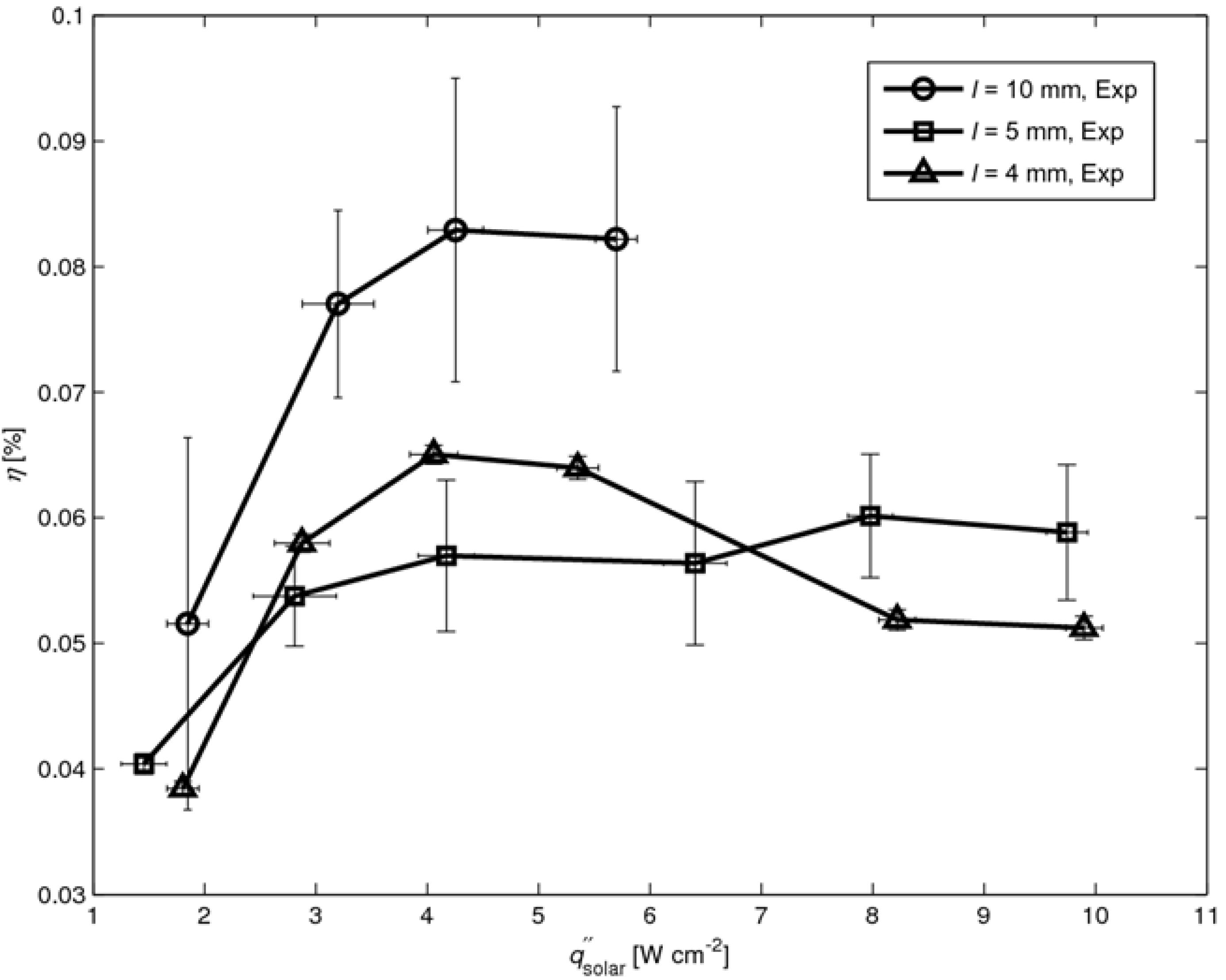
-1, respectively. The efficiency
η as a function of solar radiative flux is shown in
Figure 6 for
l = 4, 5, and 10 mm. The curves are plotted up to the maximal solar flux of 9.9, 9.7 and 5.7 W cm
-1, respectively, for which
Thot = 625°C is reached. Higher solar fluxes resulted in the burning of the graphite coating. The efficiency increases with
as a result of the higher temperature difference across the legs, which in turn corresponds to a higher Carnot limitation [
11]. In contrast,
η decreases with
T as re-radiation losses are proportional to
T4. Thus, an optimum
for maximum
η is expected. For
l = 4 mm,
ηmax = 0.065% at
= 4 W cm
-2. For
l = 5 mm
ηmax = 0.06% at
= 8 W cm
-2. For
l = 10 mm,
ηmax = 0.083% at
= 4 W cm
-2.
Figure 6.
Efficiency η as a function of solar radiative flux for three modules with l = 4, 5, and 10 mm. Error bars indicating uncertainty of incident solar radiative flux and efficiency due to uncertain contact resistance.
Figure 6.
Efficiency η as a function of solar radiative flux for three modules with l = 4, 5, and 10 mm. Error bars indicating uncertainty of incident solar radiative flux and efficiency due to uncertain contact resistance.
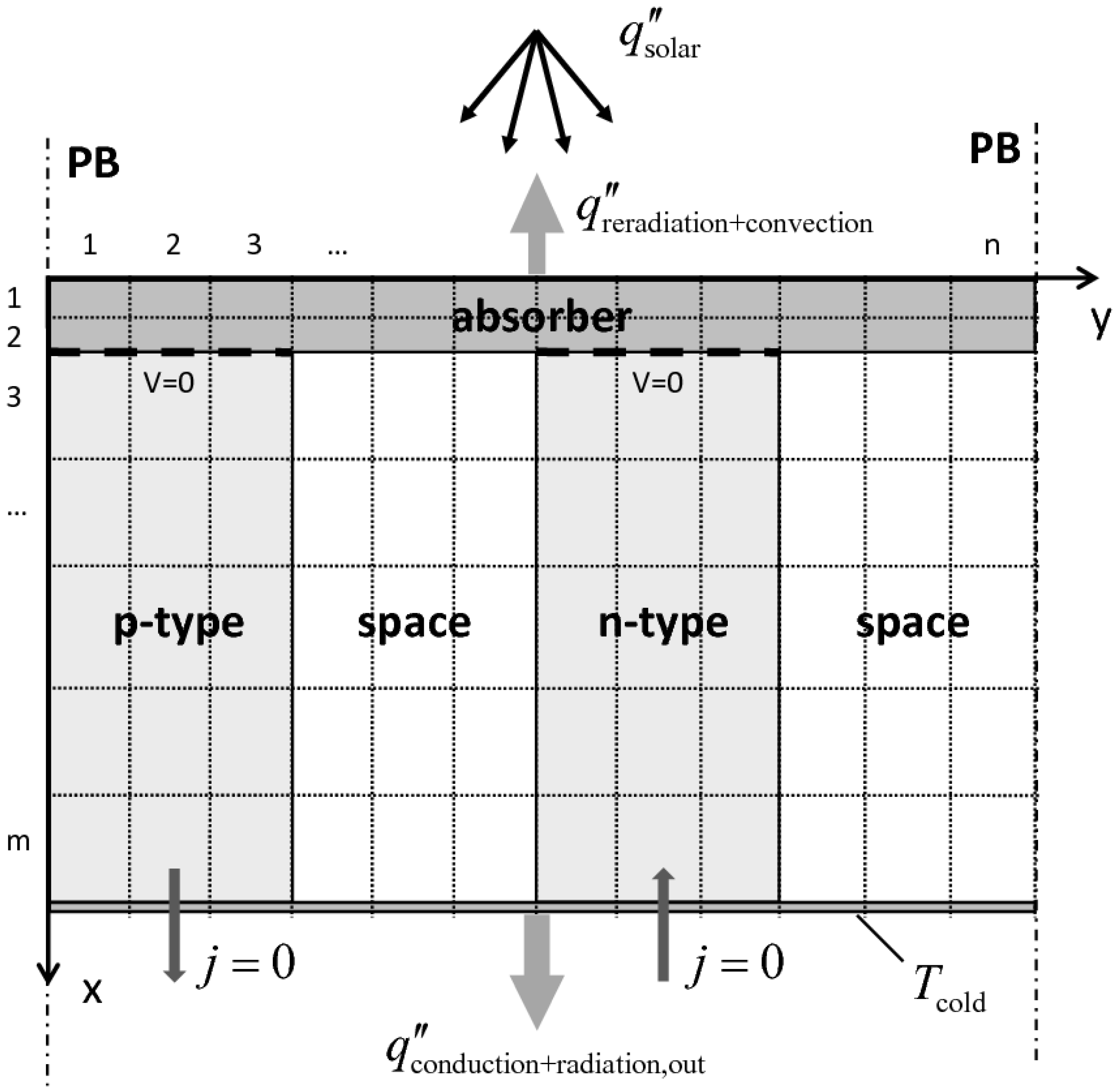
3. Heat Transfer Model
A 2D steady-state heat transfer model is formulated. A cross section of the model domain, divided into
m ×
n cells, is depicted in
Figure 7. It contains the three major components: the absorber plate, one p- and one n-leg (P/N), and the space in-between. The domain is assumed to be infinitely long; therefore, periodic boundaries are set at the sides. The heat transfer modes considered are: (1) conduction in the complete domain, and (2) radiative heat transfer among all surfaces for two approaches: (a) assuming a semi-transparent absorber plate; (b) assuming an opaque absorber plate. It is further assumed: (
i) the p/n solids are opaque, gray and diffuse scattering; (
ii) gas phase is radiatively non-participating and its refractive index is equal to unity; (
iiia) the absorber plate is radiatively participating with isotropic scattering and with temperature and wavelength independent extinction coefficient
βabs and albedo
ωabs; (
iiib) the absorber plate is opaque, gray and diffuse scattering; (
iv) convection is only considered from top of the hot plate; (
v) open circuit voltage (
j = 0).
Pmax and
η are calculated based on the matched load assumption, given by:
where
VOC is the open circuit voltage,
Rinternal the internal resistance of the TEC module, and
Rcontact the contact resistance between legs and conduction strips.
Figure 7.
Scheme of the model domain (divided into m × n cells). Indicated are the boundary conditions.
Figure 7.
Scheme of the model domain (divided into m × n cells). Indicated are the boundary conditions.
Conservation equations ― The steady-state energy conservation equation applied to the absorber for approach (a) is given by:
where
kabsorber is the absorber thermal conductivity and
is the radiative volumetric heat source. For approach (b),
= 0 and an additional boundary condition is necessary (see subchapter “boundary conditions”). The steady-state conservation equations applied to the legs (P/N domain) are given by:
with thermal conductivity
kleg, electrical resistivity
ρleg, current per area
j, and Seebeck coefficient
Sleg. Note that the two current terms cancel due to the open circuit condition:
with electrical resistivity
ρleg, chemical potential
μleg, and the charge of charged particles of current
eleg and Seebeck coefficient
Sleg [
11]. Note that the gradient of
cancels as this term is assumed constant.
For approach (a), the radiative heat transfer within the absorber plate is determined by the collision-based Monte Carlo (MC) method [
17]. The radiative source term
is approximated by:
where
qray is the power carried by a single ray,
Nabsorbed the number of rays absorbed within a control volume
∆V,
βabsorber the extinction coefficient, and
ωabsorber its albedo. Thus, the net radiative flux
of the surfaces is calculated as:
where
qray is the power carried by a single ray,
Nabsorbed the number of rays absorbed within a control surface
∆A, and ε
surface its emissivity. For approach (b), the net radiative flux
from inner surface elements is computed using the radiosity method (enclosure theory) [
18], assuming p/n-type surfaces with emissivity ε
P, ε
N, respectively, and uncoated (white) surfaces from absorber and cold plates with emissivity ε
absorber. The corresponding system of equations is given by [
17]:
where
δ is the Kronecker function,
mP/N is the number of p/n-type elements in x-direction and
nspace the number of elements in y-direction. The view factors
Fk-j are calculated by applying reciprocity relations (
A1F1-2=
A2F2-1), enclosure criterion (
), and tabulated view factors [
19].
For simplicity, 2D geometry is considered. As the total absorber surface per leg must be the same for 3D and 2D geometries, the distance d between the legs for 3D is transformed to d* for 2D. Similarly, the thermal conductivity in the direction along the plate is as adjusted as .
Boundary conditions ―
from the HFSS is assumed to be uniformly distributed. The heat losses from the absorber’s top include re-radiation and free convection. Re-radiation is calculated by MC for approach (a), and by introducing a new boundary condition for approach (b):
. Free convection
to the environment is calculated using a Nusselt correlation for a horizontal flat plate [
20]:
where Nu, Ra, Gr, and Pr are the Nusselt, Rayleigh, Grashof, and Prandtl numbers,
g the gravitational acceleration,
β the volumetric thermal expansion coefficient, ν the kinematic viscosity, α the thermal diffusity,
Tsurface the surface temperature,
T∞ the surroundings temperature, and
L the characteristic length (here the absorber width,
L = 30 mm). The outgoing heat flux contains radiation losses
through the space to the cold plate as well as conduction losses
through the legs to the cold plate.
is either calculated by MC for approach (a), and by the radiosity method for approach (b).
Numerical solution ― The finite volume technique (FV) is applied to discretize the governing equations (3) and (4) and solve the PDE system iteratively using the successive over-relaxation (SOR) method [
21] implemented in FORTRAN. The algorithm is repeated until the convergence criterion:
for all elements
i,
j after γ iterations is satisfied, with ε < 10
-6 and the overall energy balance satisfied within 0.1%. After convergence, the potential distribution is calculated. A convergence study indicated optimal trade-off between accuracy and computational time with a grid containing 425 elements.
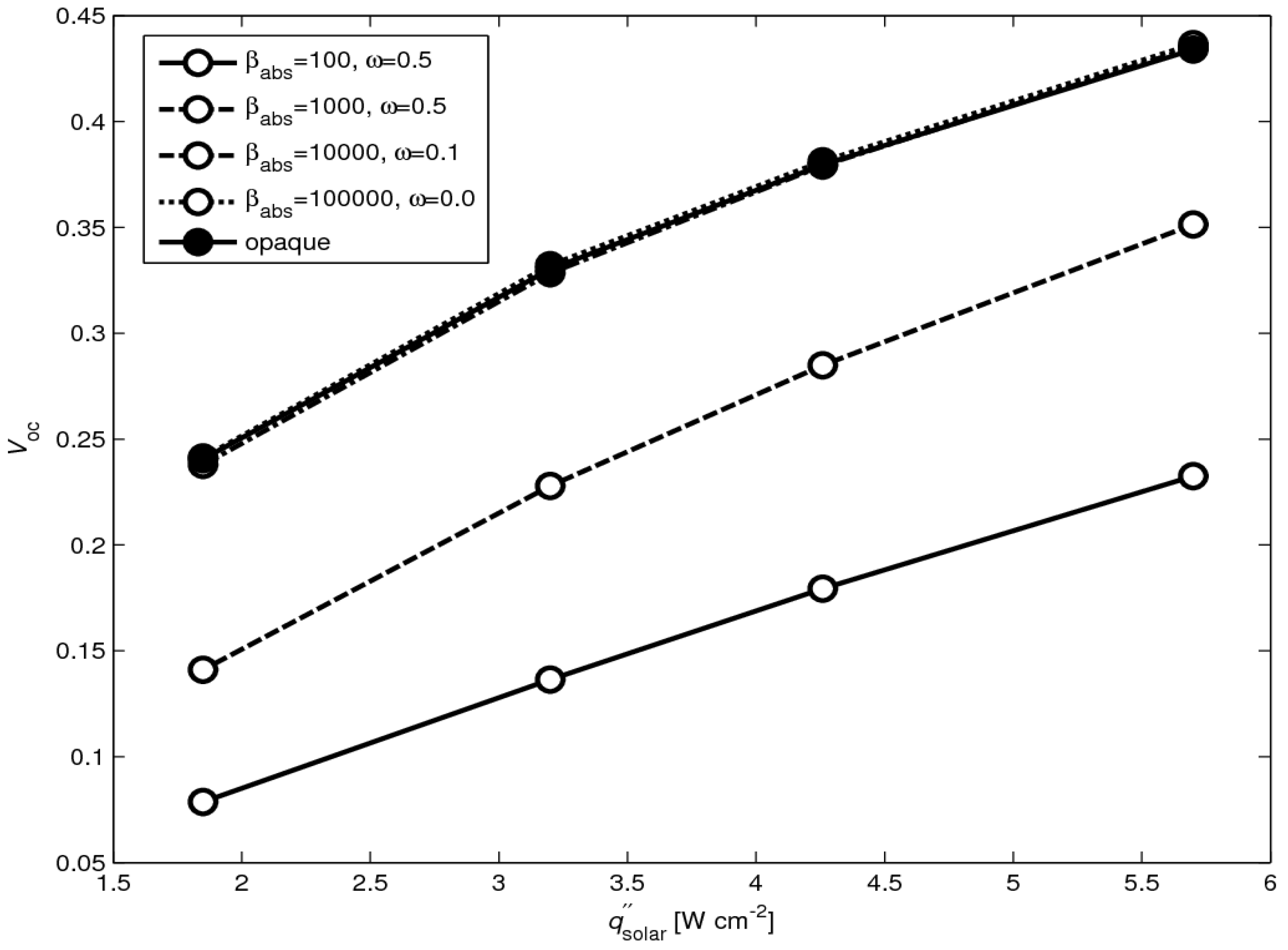
The difference between the
VOC calculated by the two approaches (a) and (b) for analyzing the radiative heat transfer is shown in
Figure 8 for
l = 10 mm. Different radiation properties (
βabs,
ω) of the absorber plate have been tested. For
βabs➔∞ and
ω➔0, no incoming radiation is transmitted through the absorber, and the solution obtained by approach (a) moves toward that for an opaque absorber obtained by approach (b). Since the absorber plate used in the measurements can be well approximated by an opaque surface, only approach (b) is applied in the analysis that follows.
Figure 8.
Simulated VOC as a function of solar radiative flux for l = 10 mm for approach (a) with βabsorber = 100, ω = 0.5; βabsorber = 1000, ω = 0.5; βabsorber = 10000, ω = 0.1; βabsorber = 100000, ω = 0.0 and for opaque approach (b).
Figure 8.
Simulated VOC as a function of solar radiative flux for l = 10 mm for approach (a) with βabsorber = 100, ω = 0.5; βabsorber = 1000, ω = 0.5; βabsorber = 10000, ω = 0.1; βabsorber = 100000, ω = 0.0 and for opaque approach (b).
4. Model Validation
Validation is accomplished for the open circuit voltage
Voc, as this value is the most reliable magnitude to measure and is directly proportional to the mean temperature difference across the legs. The baseline parameter used for the model simulations are listed in
Table 1.
Table 1.
Baseline parameters.
Table 1.
Baseline parameters.
| Parameter | Value | Unit | Source |
|---|
| l | 4 - 15 | mm | measured/varied |
| a | 3 - 6 | mm | measured/varied |
| d | 1 - 10 | mm | measured/varied |
| εabsorber,coated | 0.95 | - | [22] |
| εabsorber | 0.3 | - | [22] |
| εP/N | 0.7 | - | assumed |
| βabsorber | 100 - 100000 | m-1 | varied |
| ω | 0.0 - 0.5 | - | varied |
| k*absorber | 250 | W m-1 K-1 | assumed |
| kabsorber | 1.78 × 10⁻¹¹T4–9.79 × 10⁻⁸T3+2.02 × 10⁻⁴T2–1.90 × 10⁻¹T+75.77 | W m-1 K-1 | [23] |
| kP/N | ~ 1 – 2.5/~ 1.75 – 3 | W m-1 K-1 | measured |
| SP/N | ~ 120 – 260/~ -170 – -230 | μV K-1 | measured |
| ρP/N | ~ 0.025 - 0.05/~ 0.02 – 0.036 | Ω cm | measured |
| T∞ | 300 | K | assumed |
| Tcold | 300 | K | assumed |
| Rcontact | 0.40-0.66 | Ω | [12]/assumed |
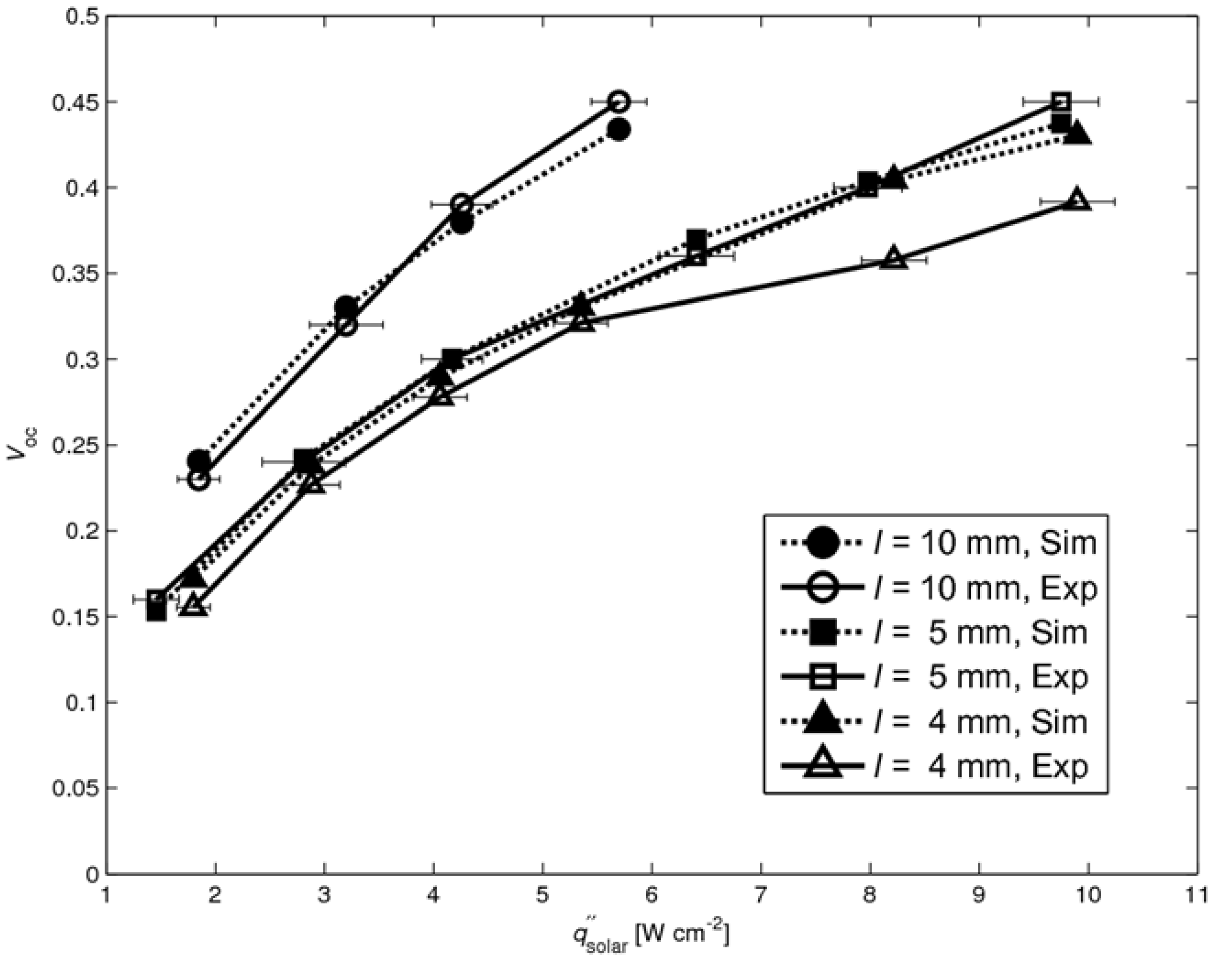
The experimentally measured and numerically calculated
VOC are shown in
Figure 9 for
l = 4, 5, and 10 mm. A reasonable good agreement is observed, except for the 4 mm case at high fluxes (
> 8 W cm
-2), where the model predicts a 15% higher value. This discrepancy is attributed to the insufficient cooling of the cold plate at high fluxes, as evidenced by a rise of its temperature, which in turn caused higher absorber plate temperature and, consequently, higher re-radiation losses. Thus, the temperature difference across the legs is shifted to higher temperatures and reduced due to the higher re-radiation.
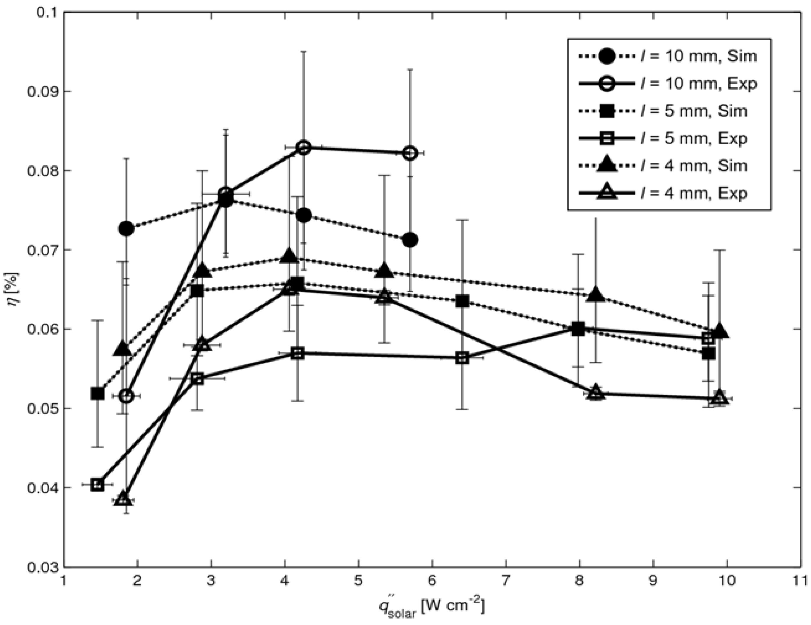
The numerically simulated solar-to-power efficiencies are shown in
Figure 10 (together with the experimentally determined efficiencies from
Figure 6), calculated using Equation (1) with maximal power output
Pmax from Equation (2). The internal leg resistances
Rinternal are calculated according to:
where
ρleg,i is the leg’s temperature dependent electrical resistivity,
Δx the cell length in x-direction,
a the width of the leg and
i the index of summation over the number of cells in x-direction along the leg (see
Figure 7). The mean contact resistance is assumed to be 0.53 ± 0.13 Ω for all cases, determined in [
12]. The calculated values lie in the same range as the measured ones, expect for the 4 mm case at high fluxes (
>8 W cm
-2) which result from the overestimated
VOC (see
Figure 9).
Figure 9.
Simulated and experimental VOC as a function of solar radiative flux for l = 4, 5, 10 mm. Error bars indicating uncertainty of incident solar radiative flux.
Figure 9.
Simulated and experimental VOC as a function of solar radiative flux for l = 4, 5, 10 mm. Error bars indicating uncertainty of incident solar radiative flux.
Figure 10.
Simulated and experimental
η as a function of solar radiative flux for
l = 4, 5, 10 mm (experimental data from
Figure 6). Error bars for simulated data points indicating uncertainty of contact resistance.
Figure 10.
Simulated and experimental
η as a function of solar radiative flux for
l = 4, 5, 10 mm (experimental data from
Figure 6). Error bars for simulated data points indicating uncertainty of contact resistance.
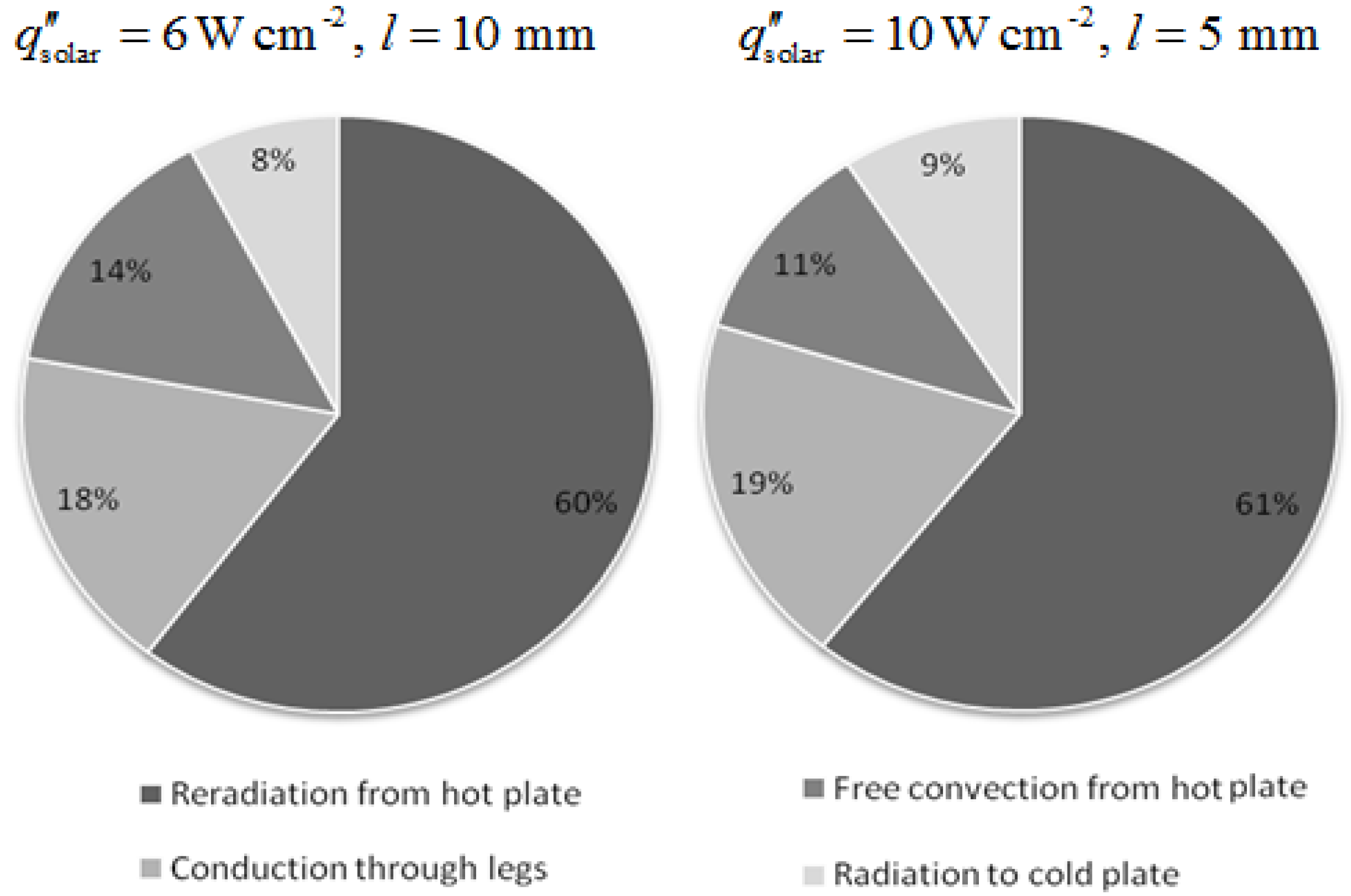
The percentage of
Qsolar transferred by the different heat transfer modes is shown in
Figure 11 for two cases; 1)
= 6 W cm
-2 and
l = 10 mm leg length, and 2)
= 10 W m
-2 and
l = 5 mm. In both cases, the heat losses by re-radiation and free convection from the absorber plate represent more than 70% of
Qsolar. About 20% of
Qsolar is transferred by conduction through the legs, and <10% is lost by radiation to the cold plate.
Figure 11.
Percentage of Qsolar transferred by the heat transfer modes.
Figure 11.
Percentage of Qsolar transferred by the heat transfer modes.
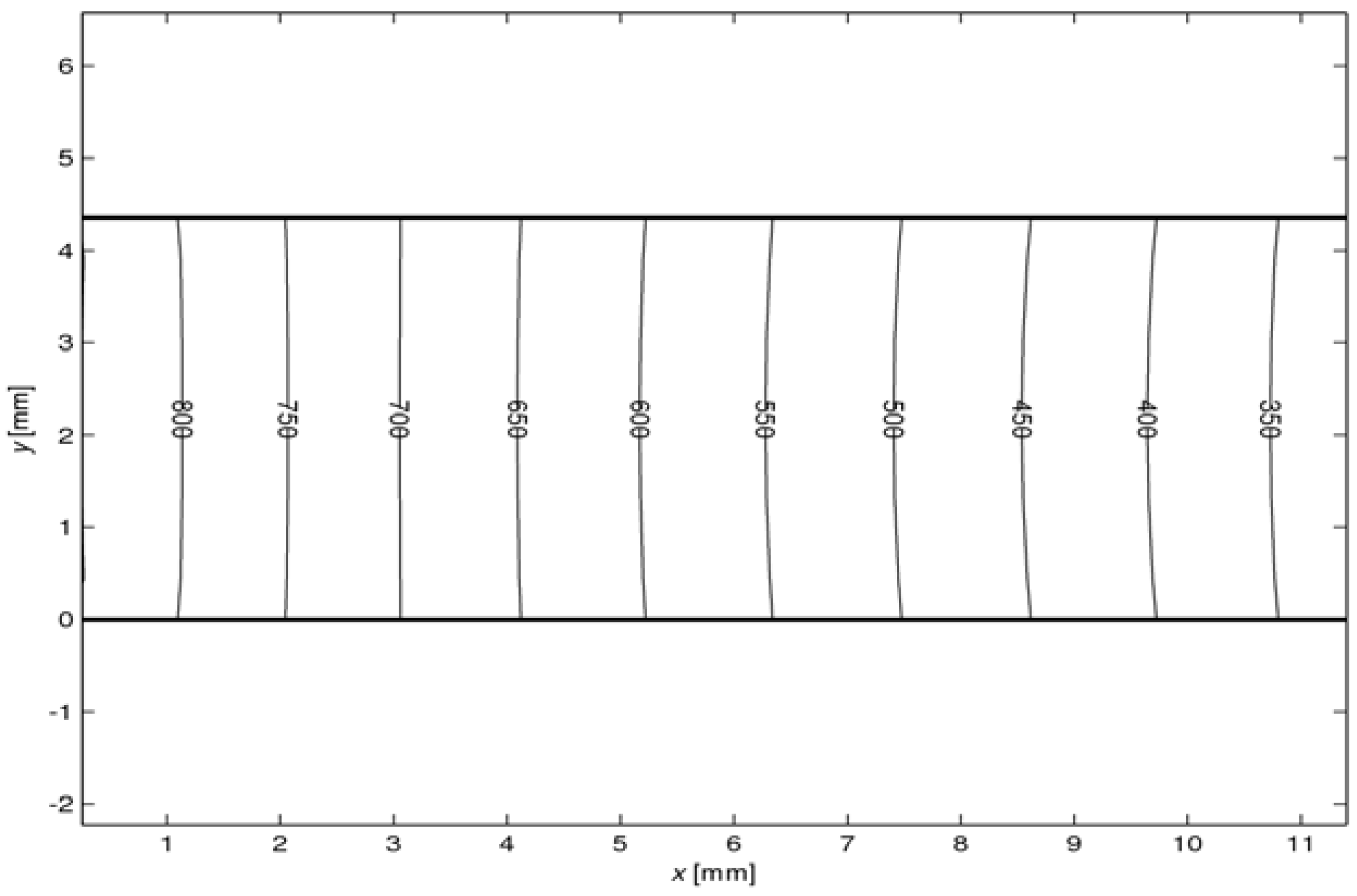
Figure 12 shows the temperature distribution along a p-type leg of
l = 10 mm obtained for
= 6 W m
-2. A comparable distribution is obtained for an n-type leg. The profile is linear, as corroborated by the experimental data (see
Figure 5). Perpendicular to the length axis, the temperature is almost uniform, with a slightly higher temperature at the surface because of the radiative exchange among legs and plates. The small temperature gradient indicates that this radiative heat exchange is not predominant, as confirmed by the fact that <10% of
Qsolar is lost by radiation to the cold plate (see
Figure 11).
Figure 12.
2D temperature profile in p-type leg for l = 10 mm at = 6 W m-2.
Figure 12.
2D temperature profile in p-type leg for l = 10 mm at = 6 W m-2.
5. Efficiency
Leg length ―The simulated dimensions of the modules are
l = 5 - 15 mm,
a = 4.5 mm, and plates with
Lx
Lx
b = 30 × 30 × 0.25 mm. The cold plate temperature is set to 300 K. The contact resistance is
RContact = 0.55 Ω. The solar radiative fluxes are varied in the range
. The black coating of the absorber is assumed stable for all temperatures. The baseline parameter used for the model simulations are listed in
Table 1.
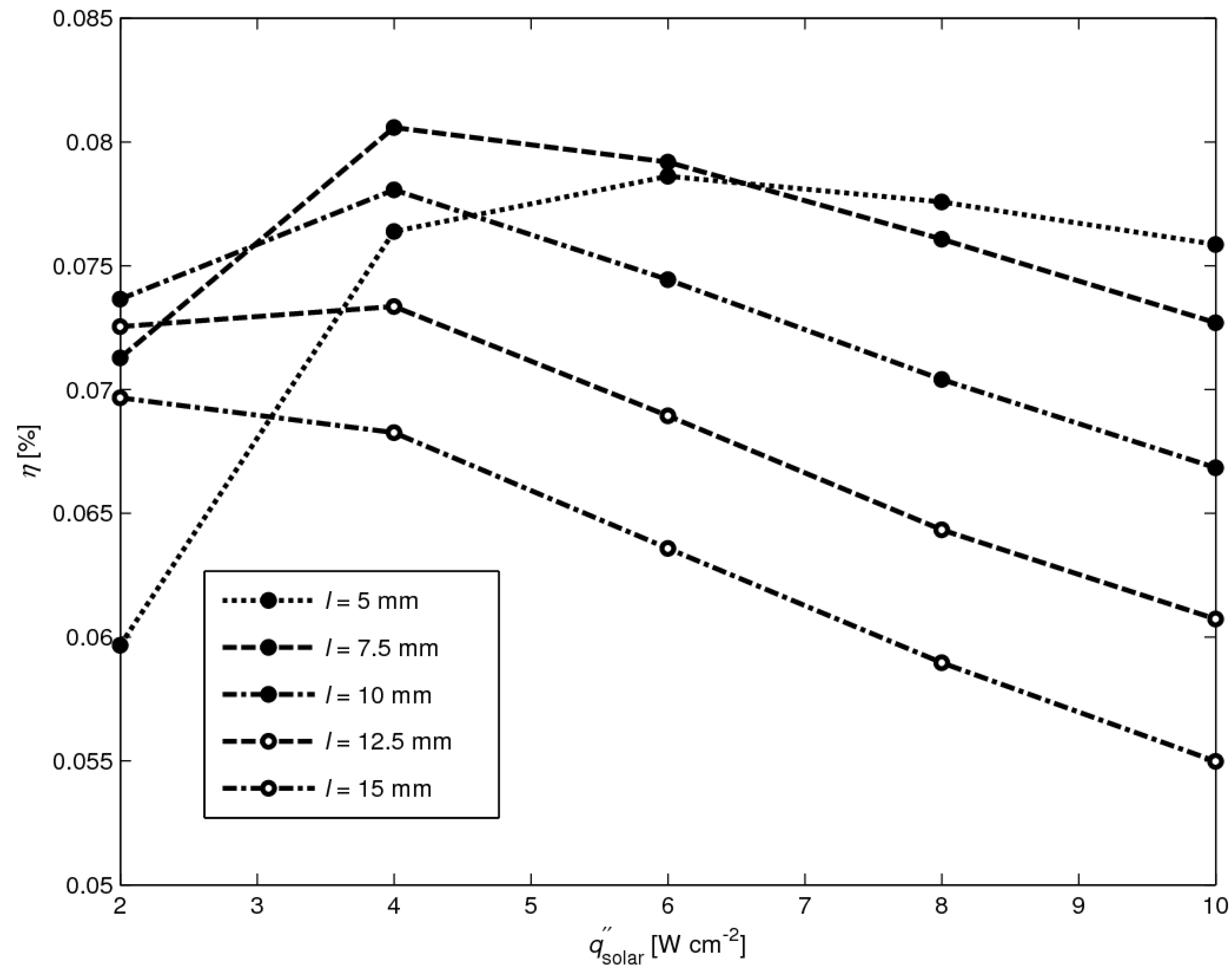
Figure 13 shows the efficiency as a function of solar radiative flux for
l = 5, 7.5, 10, 12.5 and 15 mm. The highest efficiency
η = 0.081% is obtained for
l = 7.5 mm at
= 4 W cm
-2. Note that
l = 7.5 mm is not optimal in the whole solar radiative flux range. For
< 3 W cm
-2,
l = 10 mm is most efficient, whereas for
> 7 W cm
-2,
l = 5 mm is most efficient. Thus, for increasing solar radiative fluxes, the optimal leg length decreases.
Figure 13.
Efficiency as a function of solar radiative flux for l = 5 mm, l = 7.5 mm, l = 10 mm, l = 12.5 mm and l = 15 mm.
Figure 13.
Efficiency as a function of solar radiative flux for l = 5 mm, l = 7.5 mm, l = 10 mm, l = 12.5 mm and l = 15 mm.
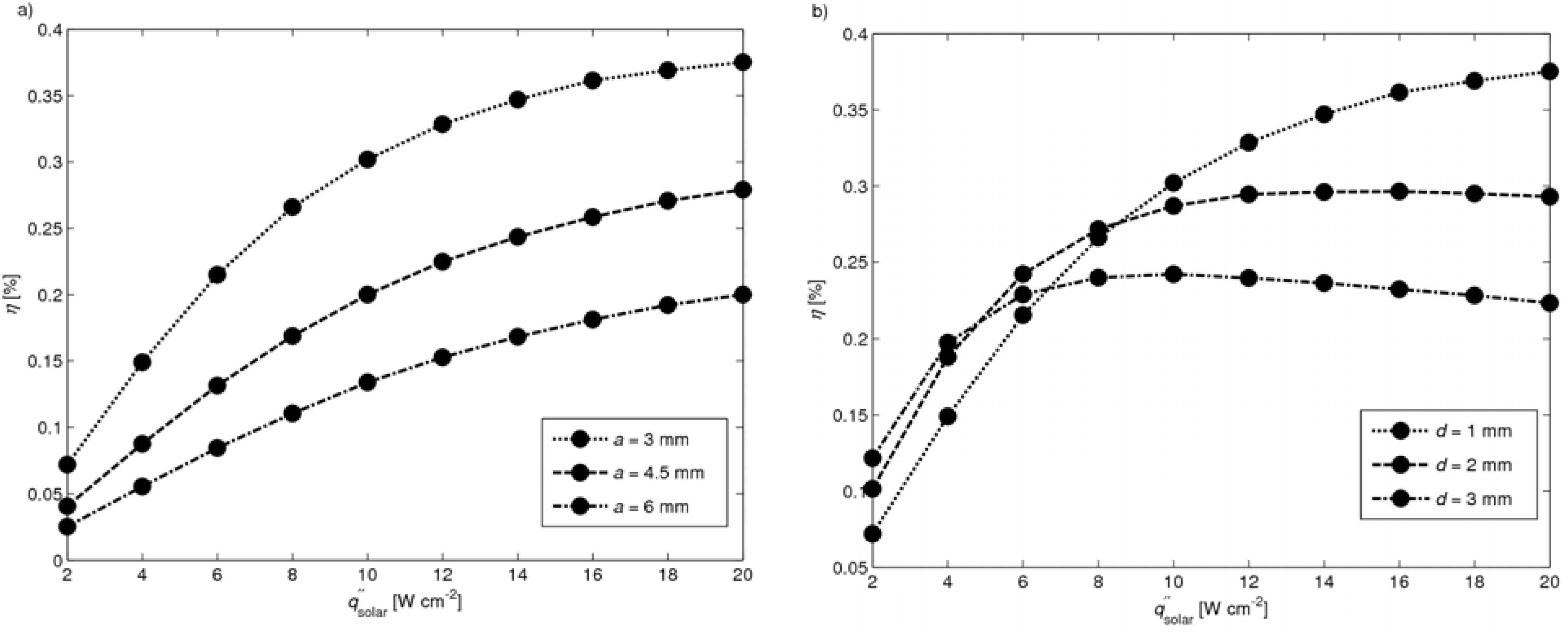
Leg width and distance between neighboring legs ― For practical manufacturing purposes, it is assumed that the minimal leg width is
a = 3 mm and the minimal distance
d = 1 mm. In
Figure 14, the efficiencies are plotted as a function of solar radiative flux in the range
= 2 – 20 W cm
-1 for a module with a leg length
l = 7.5 mm and for: (a)
d = 1 mm and
a = 3, 4.5, 6 mm, and (b)
a = 3 mm and
d = 1, 2, 3 mm. Highest efficiencies are obtained for
a = 3 mm in the whole solar flux range, and for
d = 1 mm in the range
= 8 – 20 W cm
-2. The peak
η = 0.375% at
= 20 W cm
-2 is obtained for
a = 3 mm and
d = 1 mm,
i.e. for the smallest leg width and distance between neighboring legs considered.
Figure 14.
Efficiency as a function of solar radiative flux with l = 7.5 mm for (a) d = 1 mm and a = 3, 4.5, 6 mm and for (b) a = 3 mm and d = 1, 2, 3 mm.
Figure 14.
Efficiency as a function of solar radiative flux with l = 7.5 mm for (a) d = 1 mm and a = 3, 4.5, 6 mm and for (b) a = 3 mm and d = 1, 2, 3 mm.


