
An Adaptive Hybrid Correlation Kriging Approach for Uncertainty Dynamic Optimization of Spherical-Conical Shell Structure


Abstract
1. Introduction
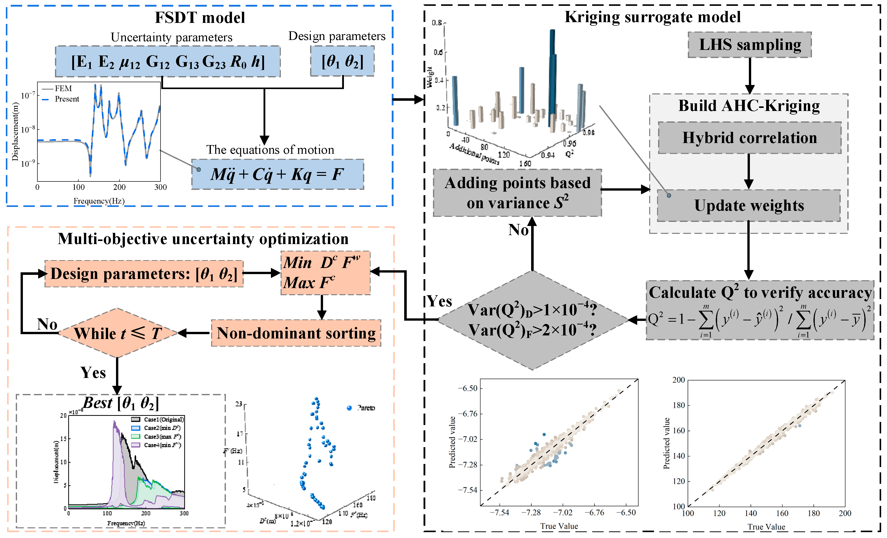
2. Dynamic Model of the Spherical-Conical Shell
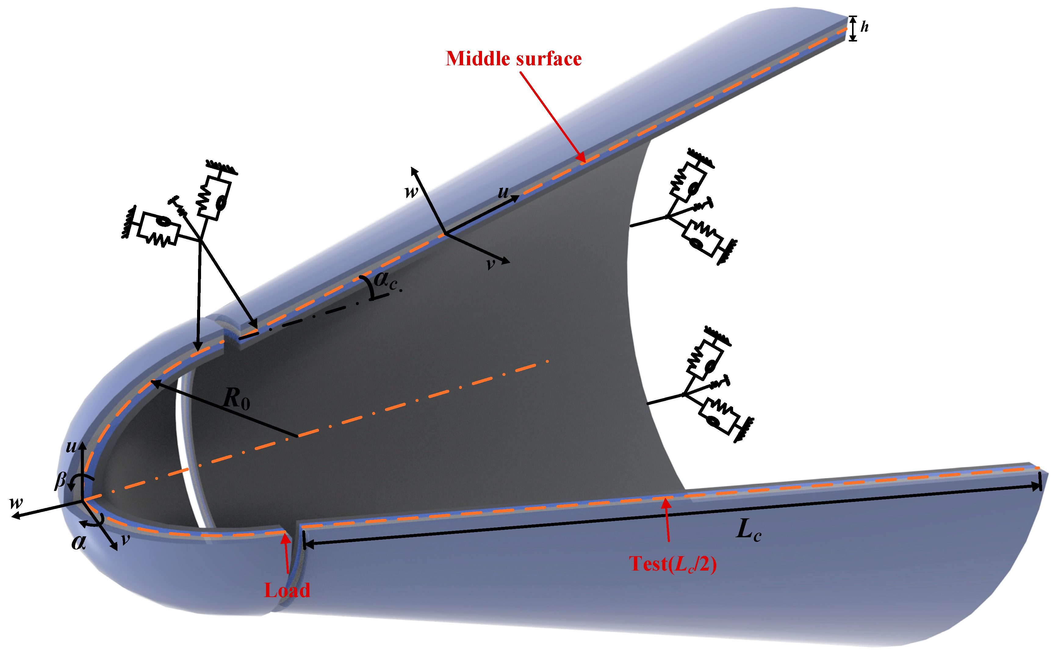
2.1. Description of the Structure
2.2. Equations of Motion for Vibrational Characterization
2.3. Dynamic Model Verification
3. Adaptive Hybrid Correlation Kriging Analysis
3.1. The Introduction to the Correlation Functions
3.2. Improved Strategy of AHC-Kriging
3.3. Performance Analysis of AHC-Kriging
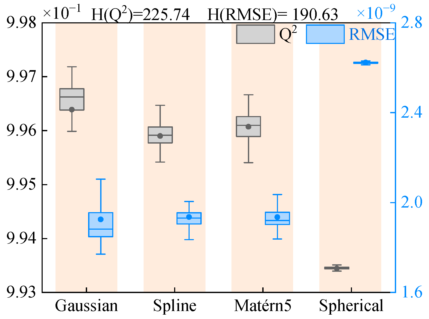
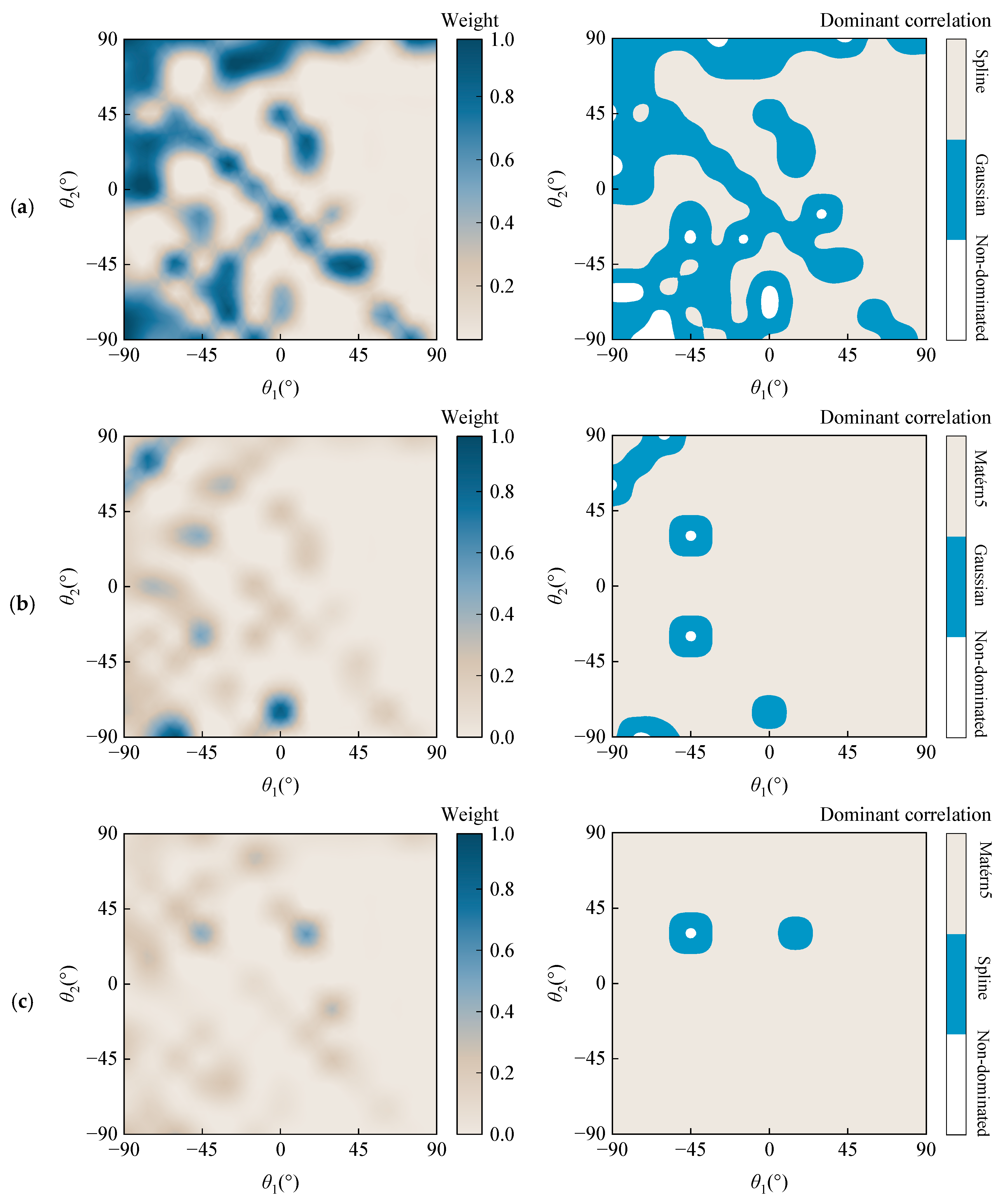
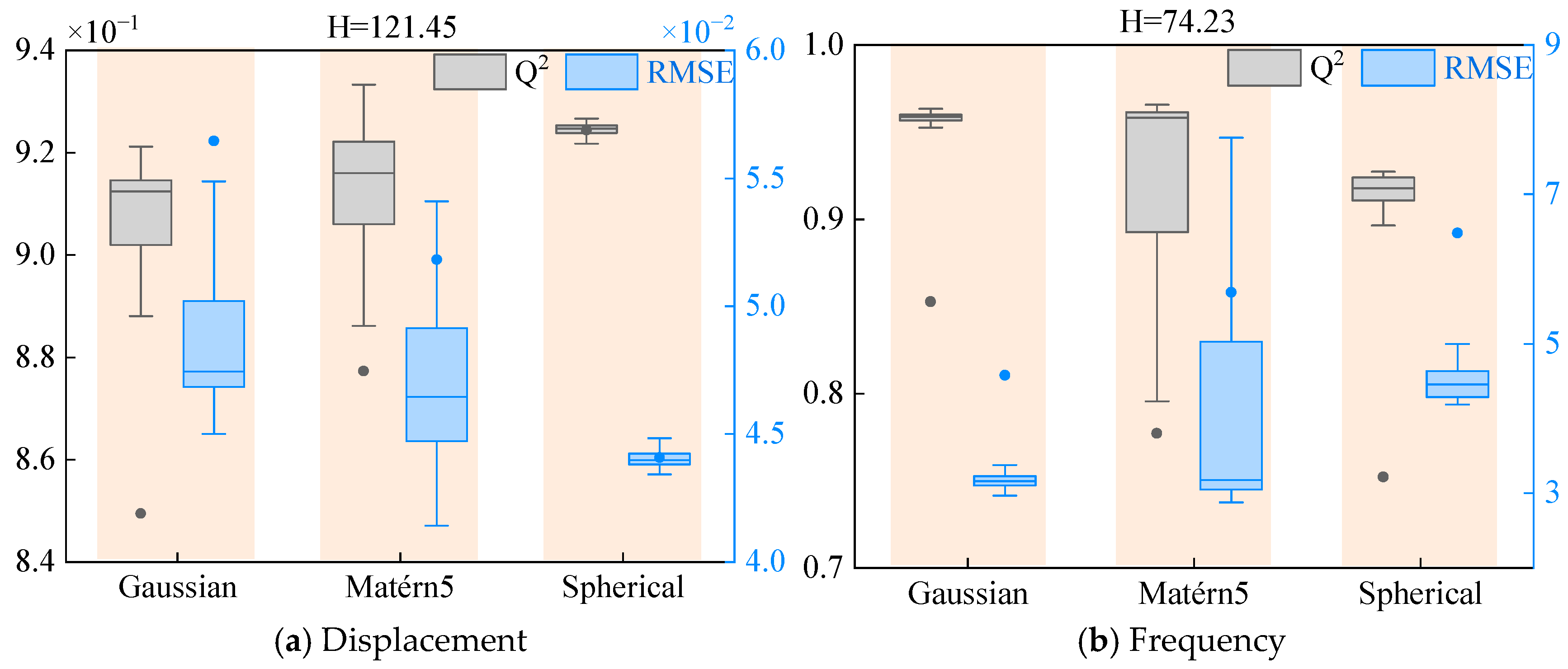
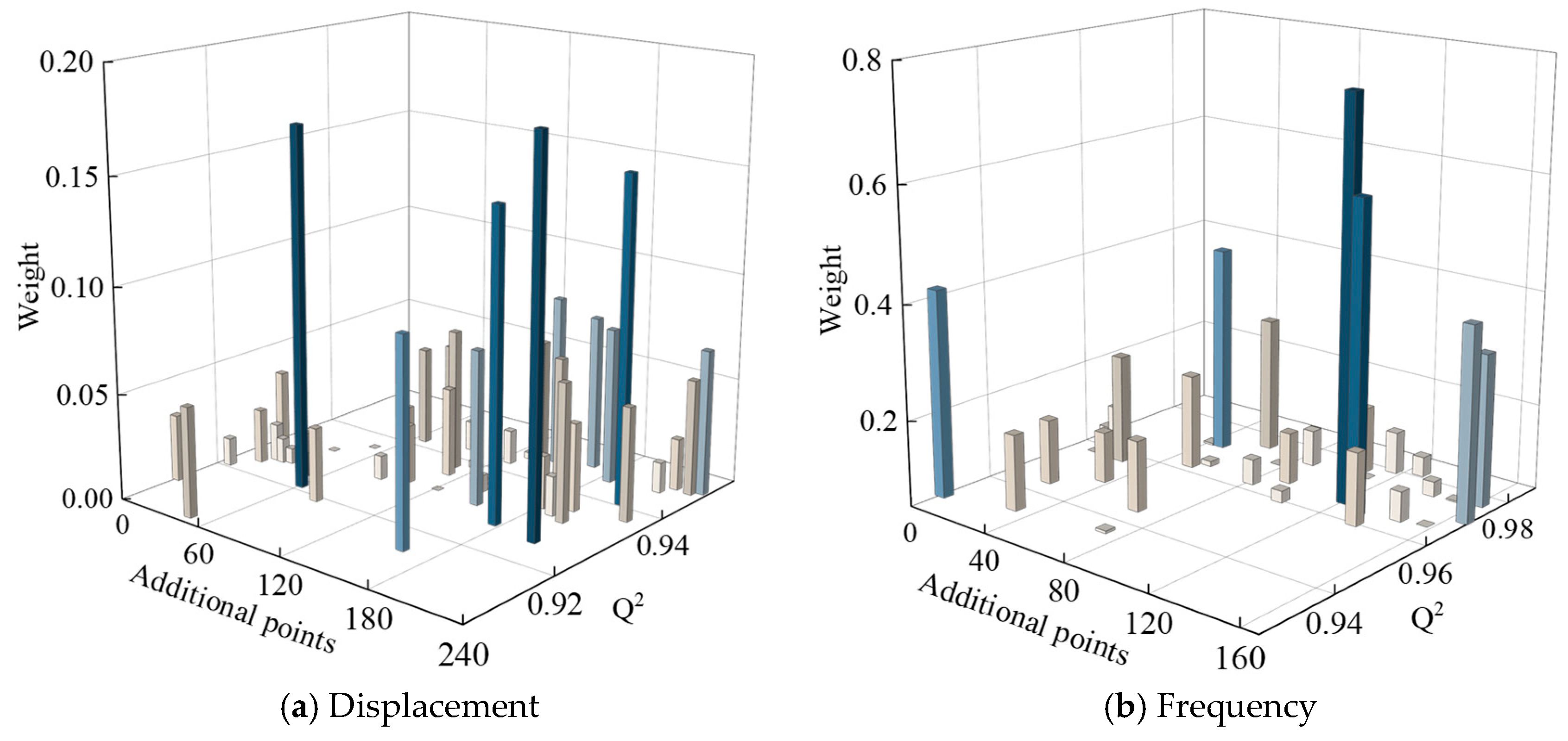
3.4. Weighting Analysis Based on AHC-Kriging
4. Uncertainty Optimization of the Spherical-Conical Shell
4.1. Problem Statement for Optimization with Parametric Uncertainties
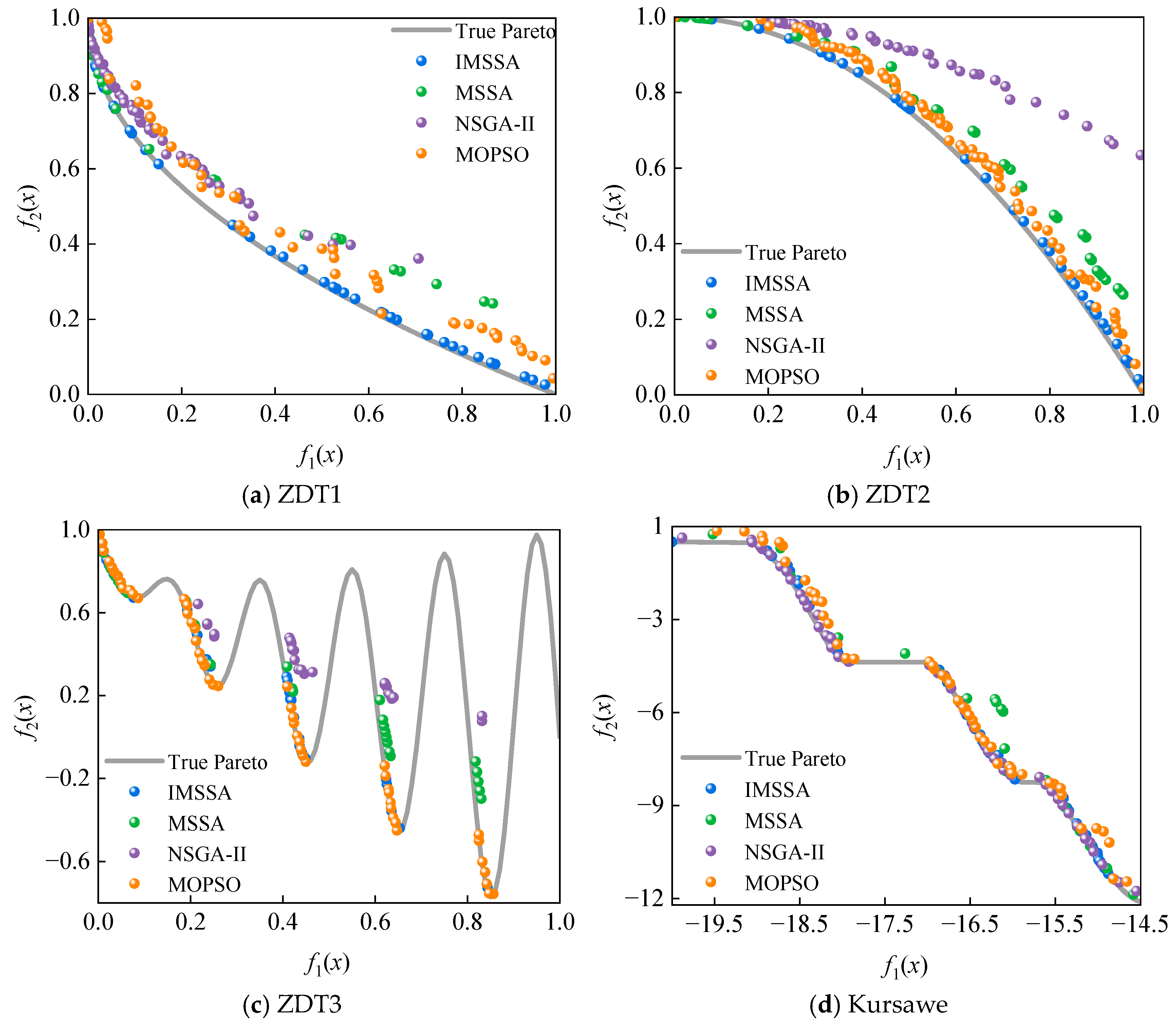
4.2. Improved Multi-Objective Salp Swarm Algorithm
| Algorithm 1. The overall process of the IMSSA |
| Pseudo code: IMSSA |
| Set problem parameters: population size (N), iterations (T), number of objectives, dimensions, and upper and lower bounds. Randomly generate the initial salp population. Evaluate the objective function. for t = 1: T do for i = 1: N do Evaluate the objective function. Update the position of food(F) in the current population. end for Update the repository. Chose the repository member in the least population area as food(F). for i = 1: N do if i < N/2 Update the position of the leader based on Equation (28). else Update the position of the followers based on Equations (30) and (31). end if Correct for the salps based on the upper and lower bounds of variables. end for end for Return repository. |
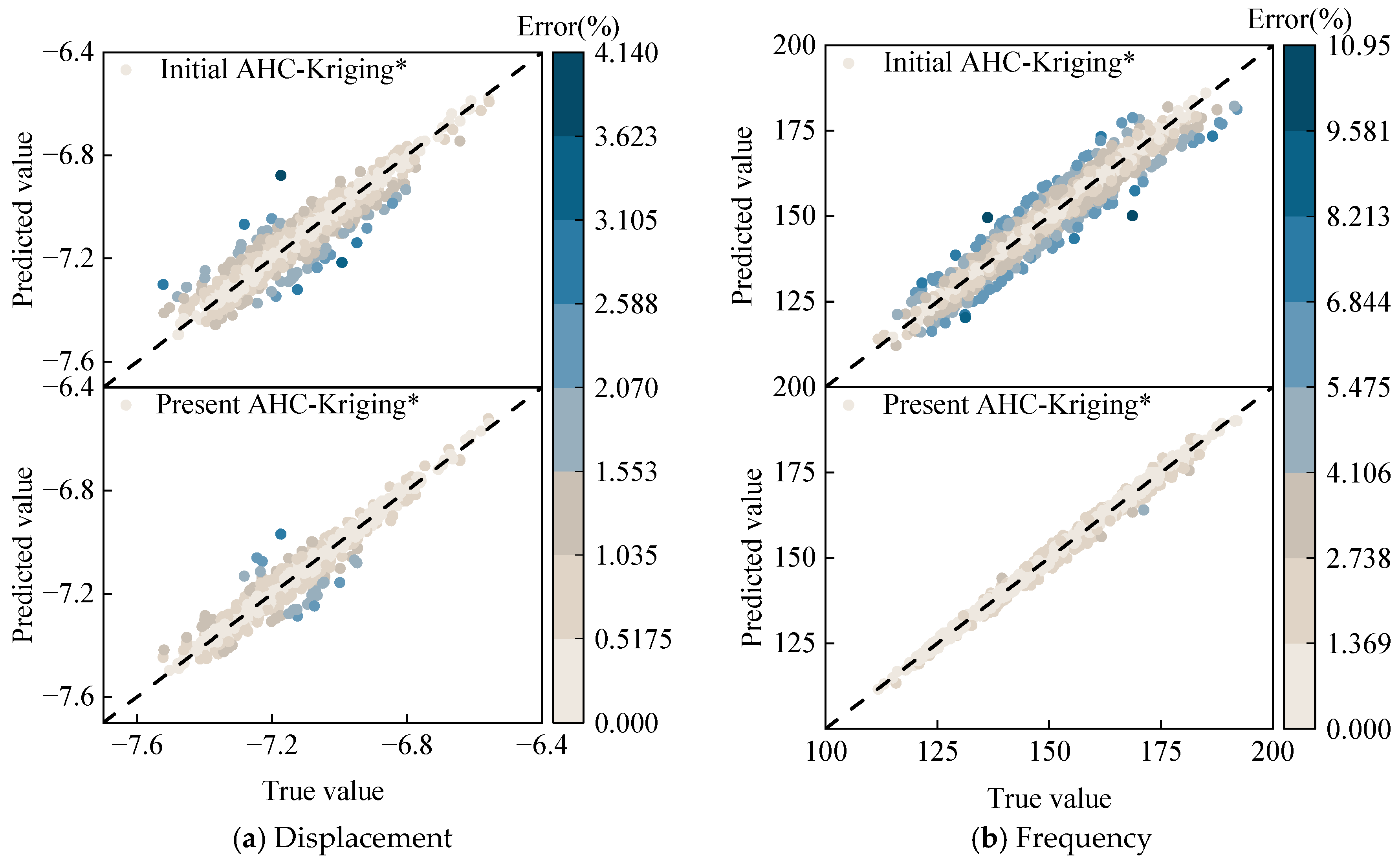
4.3. Validation of AHC-Kriging for Uncertainty Optimization
4.4. Optimization Analysis
5. Conclusions
Author Contributions
Funding
Institutional Review Board Statement
Informed Consent Statement
Data Availability Statement
Acknowledgments
Conflicts of Interest
References
- Alkbir, M.F.M.; Sapuan, S.M.; Nuraini, A.A.; Ishak, M.R. Fibre properties and crashworthiness parameters of natural fibre-reinforced composite structure: A literature review. Compos. Struct. 2016, 148, 59–73. [Google Scholar] [CrossRef]
- Fernandes, P.; Pinto, R.; Correia, N. Design and optimization of self-deployable damage tolerant composite structures: A review. Compos. Part B Eng. 2021, 221, 109029. [Google Scholar] [CrossRef]
- Savchenko, E.V. Evolutionary Algorithms in the Problems of Structure Optimization for Composite Shells from Viscoelastic Materials. Strength Mater. 2013, 45, 192–198. [Google Scholar] [CrossRef]
- Irisarri, F.X.; Abdalla, M.M.; Guerdal, Z. Improved Shepard’s Method for the Optimization of Composite Structures. AIAA J. 2011, 49, 2726–2736. [Google Scholar] [CrossRef]
- Melih, S.; Levent, A. Stochastic optimization of graphite-flax/epoxy hybrid laminated composite for maximum fundamental frequency and minimum cost. Eng. Struct. 2018, 174, 675–687. [Google Scholar]
- Khatir, A.; Capozucca, R.; Khatir, S.; Magagnini, E.; Cuong-Le, T. Enhancing Damage Detection Using Reptile Search Algorithm-Optimized Neural Network and Frequency Response Function. J. Vib. Eng. Technol. 2025, 13, 88. [Google Scholar] [CrossRef]
- Khatir, A.; Capozucca, R.; Khatir, S.; Magagnini, E.; Benaissa, B.; Cuong-Le, T. An efficient improved Gradient Boosting for strain prediction in Near-Surface Mounted fiber-reinforced polymer strengthened reinforced concrete beam. Front. Struct. Civ. Eng. 2024, 18, 1148–1168. [Google Scholar] [CrossRef]
- Osmani, A.; Shamass, R.; Tsavdaridis, K.D.; Ferreira, F.P.V.; Khatir, A. Deflection Predictions of Tapered Cellular Steel Beams Using Analytical Models and an Artificial Neural Network. Buildings 2025, 15, 992. [Google Scholar] [CrossRef]
- Khatir, A.; Capozucca, R.; Khatir, S.; Magagnini, E.; Le Thanh, C.; Riahi, M.K. Advancements and emerging trends in integrating machine learning and deep learning for SHM in mechanical and civil engineering: A comprehensive review. J. Braz. Soc. Mech. Sci. Eng. 2025, 47, 419. [Google Scholar] [CrossRef]
- Hassaine, N.; Dahak, M.; Touat, N.; Khatir, S.; Benaissa, B.; Cuong-Le, T. Damage identification in functionally graded material beam structures based on frequency analysis and AOA-ANN. Mech. Based Des. Struct. Mach. 2025, 1–21. [Google Scholar] [CrossRef]
- Khatir, A.; Capozucca, R.; Khatir, S.; Magagnini, E.; Benaissa, B.; Le Thanh, C.; Abdel Wahab, M. A new hybrid PSO-YUKI for double cracks identification in CFRP cantilever beam. Compos. Struct. 2023, 311, 116803. [Google Scholar] [CrossRef]
- Wang, W.; Wang, Q.; Zhong, R.; Chen, L.; Shi, X. Stacking sequence optimization of arbitrary quadrilateral laminated plates for maximum fundamental frequency by hybrid whale optimization algorithm. Compos. Struct. 2023, 310, 116764. [Google Scholar] [CrossRef]
- Chen, Y.; Shao, Y.; Xiao, X. A new method for predicting the morphology and surface roughness of micro grooves in aluminum alloy ablated by pulsed laser. J. Manuf. Process. 2023, 96, 193–203. [Google Scholar] [CrossRef]
- Dat, N.D.; Quan, T.Q.; Duc, N.D. Nonlinear thermal dynamic buckling and global optimization of smart sandwich plate with porous homogeneous core and carbon nanotube reinforced nanocomposite layers. Eur. J. Mech. A/Solids 2021, 90, 104351. [Google Scholar] [CrossRef]
- Duc, N.D.; Foroutan, K.; Varedi-Koulaei, S.M.; Ahmadi, H. Nonlinear Vibration Analysis of Laminated Composite Cylindrical Shell Under External Loading Utilizing Meta-Heuristic Optimization Algorithms. Iran. J. Sci. Technol. Trans. Mech. Eng. 2024, 48, 757–777. [Google Scholar] [CrossRef]
- Peng, X.; Guo, Y.; Qiu, C.; Wu, H.; Li, J.; Chen, G.; Jiang, S.; Liu, Z. Reliability optimization design for composite laminated plate considering multiple types of uncertain parameters. Eng. Optim. 2021, 53, 221–236. [Google Scholar] [CrossRef]
- Naskar, S.; Mukhopadhyay, T.; Sriramula, S. Probabilistic micromechanical spatial variability quantification in laminated composites. Compos. Part B Eng. 2018, 151B, 291–325. [Google Scholar] [CrossRef]
- Mukhopadhyay, T.; Naskar, S.; Chakraborty, S.; Karsh, P.K.; Dey, S. Stochastic Oblique Impact on Composite Laminates: A Concise Review and Characterization of the Essence of Hybrid Machine Learning Algorithms. Arch. Comput. Methods Eng. 2020, 28, 3. [Google Scholar] [CrossRef]
- Young, R.C. The algebra of many-valued quantities. Math. Ann. 1931, 104, 260–290. [Google Scholar] [CrossRef]
- Sengupta, A.; Pal, T.K.; Chakraborty, D. Interpretation of inequality constraints involving interval coefficients and a solution to interval linear programming. Fuzzy Sets Syst. 2001, 119, 129–138. [Google Scholar] [CrossRef]
- Krige, D.G. A Statistical Approach to Some Mine Valuation and Allied Problems on the Witwatersrand; University of the Witwatersrand: Johannesburg, South Africa, 1951. [Google Scholar]
- Sakata, S.; Ashida, F.; Zako, M. Kriging-based approximate stochastic homogenization analysis for composite materials. Comput. Methods Appl. Mech. Eng. 2008, 197, 1953–1964. [Google Scholar] [CrossRef]
- Wang, W.; Wang, Q.; Zhong, R.; Shi, X.; Chen, L. Optimization of stacking sequence for quadrilateral laminated composite plates with curved edges based on Kriging. Comput. Math. Appl. 2024, 159, 142–154. [Google Scholar] [CrossRef]
- Palar, P.S.; Zuhal, L.R.; Shimoyama, K. Gaussian Process Surrogate Model with Composite Kernel Learning for Engineering Design. AIAA J. 2020, 58, 4. [Google Scholar] [CrossRef]
- Jin, S.S. Compositional kernel learning using tree-based Genetic programming for Gaussian process regression. Struct. Multidiscip. Optim. 2020, 62, 1313–1351. [Google Scholar] [CrossRef]
- Guoji, X.; Chengjie, J.; Peng, J.Y. A novel ensemble model using artificial neural network for predicting wave-induced forces on coastal bridge decks. Eng. Comput. 2023, 39, 3269–3292. [Google Scholar]
- Li, Z.; Zhang, S.; Li, H.; Tian, K.; Cheng, Z.; Chen, Y.; Wang, B. On-line transfer learning for multi-fidelity data fusion with ensemble of deep neural networks. Adv. Eng. Inform. 2022, 53, 101689. [Google Scholar] [CrossRef]
- Shang, X.; Zhang, Z.; Fang, H.; Li, B.; Li, Y. Ensemble learning of multi-kernel Kriging surrogate models using regional discrepancy and space-filling criteria-based hybrid sampling method. Adv. Eng. Inform. 2023, 58, 102186. [Google Scholar] [CrossRef]
- Chen, L.; Qiu, H.; Jiang, C.; Cai, X.; Gao, L. Ensemble of surrogates with hybrid method using global and local measures for engineering design. Struct. Multidiscip. Optim. 2018, 57, 1711–1729. [Google Scholar] [CrossRef]
- Goel, T.; Haftka, R.; Shyy, W.; Queipo, N.V. Ensemble of surrogates. Struct. Multidiscip. Optim. 2007, 33, 199–216. [Google Scholar] [CrossRef]
- Viana, F.A.C.; Haftka, R.; Steffen, V., Jr. Multiple surrogates: How cross-validation errors can help us to obtain the best predictor. Struct. Multidiscip. Optim. 2009, 39, 439–457. [Google Scholar] [CrossRef]
- Shi, R.; Liu, L.; Long, T.; Liu, J. An efficient ensemble of radial basis functions method based on quadratic programming. Eng. Optim. 2016, 48, 1202–1225. [Google Scholar] [CrossRef]
- Zerpa, L.E.; Queipo, N.V.; Pintos, S.; Salager, J.L. An optimization methodology of alkaline–surfactant–polymer flooding processes using field scale numerical simulation and multiple surrogates. J. Pet. Sci. Eng. 2005, 47, 197–208. [Google Scholar] [CrossRef]
- Acar, E. Various approaches for constructing an ensemble of metamodels using local measures. Struct. Multidiscip. Optim. 2010, 42, 879–896. [Google Scholar] [CrossRef]
- Kronberger, G.; Kommenda, M. Evolution of Covariance Functions for Gaussian Process Regression using Genetic Programming. In Proceedings of the Computer Aided Systems Theory—EUROCAST 2013: 14th International Conference, Las Palmas de Gran Canaria, Spain, 10–15 February 2013; Springer: New York, NY, USA, 2013. [Google Scholar]
- Duvenaud, D.; Lloyd, J.R.; Grosse, R.; Tenenbaum, J.B.; Ghahramani, Z. Structure Discovery in Nonparametric Regression through Compositional Kernel Search. In Proceedings of the 30th International Conference on International Conference on Machine Learning, Atlanta, GA, USA, 16–21 June 2013. [Google Scholar]
- Lloyd, J.R.; Duvenaud, D.; Grosse, R.; Tenenbaum, J.B.; Ghahramani, Z. Automatic Construction and Natural-Language Description of Nonparametric Regression Models. In Proceedings of the Twenty-Eighth AAAI Conference on Artificial Intelligence, Québec City, QC, Canada, 27–31 July 2014. [Google Scholar]
- Choe, K.; Shuai, C.; Wang, A.; Wang, Q. Free vibration analysis of laminated composite elliptic cylinders with general boundary conditions. Compos. Part B Eng. 2019, 158, 55–66. [Google Scholar]
- Kapania, R.K. Review of Vibration of Laminated Shells and Plates. AIAA J. 2004, 42, 1946–1947. [Google Scholar] [CrossRef]
- Choe, K.; Wang, Q.; Tang, J.; Shui, C. Vibration analysis for coupled composite laminated axis-symmetric doubly-curved revolution shell structures by unified Jacobi-Ritz method. Compos. Struct. 2018, 194, 136–157. [Google Scholar] [CrossRef]
- Zhong, R.; Guan, X.; Wang, Q.; Qin, B.; Shuai, C. Prediction of acoustic radiation from elliptical caps of revolution by using a semi-analytic method. J. Braz. Soc. Mech. Sci. Eng. 2021, 43, 383. [Google Scholar] [CrossRef]
- Qu, Y.; Long, X.; Wu, S.; Meng, G. A unified formulation for vibration analysis of composite laminated shells of revolution including shear deformation and rotary inertia. Compos. Struct. 2013, 98, 169–191. [Google Scholar] [CrossRef]
- Jia, D.; Gao, C.; Yang, Y.; Pang, F.; Li, H.; Du, Y. A semi-analytical method for dynamic analysis of a rectangular plate with general boundary conditions based on FSDT. Rev. Adv. Mater. Sci. 2022, 61, 477–492. [Google Scholar] [CrossRef]
- Lee, J. Free vibration analysis of joined spherical-cylindrical shells by matched Fourier-Chebyshev expansions. Int. J. Mech. Sci. 2017, 122, 53–62. [Google Scholar] [CrossRef]
- Huang, T.; Wang, Q.; Chen, L.; Zhong, R. Kriging-based uncertainty optimization of vibration characteristics for laminated elliptical shells considering material and load uncertainties. Eur. J. Mech. A/Solids 2025, 111, 105587. [Google Scholar] [CrossRef]
- Matheron, G. Principles of geostatistics. Econ. Geol. 1963, 58, 1246–1266. [Google Scholar] [CrossRef]
- Sacks, J.; Welch, W.J.; Wynn, M.H.P. [Design and Analysis of Computer Experiments]: Rejoinder. Stat. Sci. 1989, 4, 433–435. [Google Scholar] [CrossRef]
- Matlab, A.; Toolbox, K.; Lophaven, S.N.; Nielsen, H.B.; Sndergaard, J. DACE—A MATLAB Kriging Toolbox. 2002. Available online: https://www.omicron.dk/dace.html (accessed on 1 June 2025).
- Kruskal, W.H.; Wallis, W.A. Use of ranks in one-criterion variance analysis. J. Am. Stat. Assoc. 1952, 47, 583–621. [Google Scholar] [CrossRef]
- Jiang, C.; Han, X.; Liu, G.R.; Liu, G.P. A nonlinear interval number programming method for uncertain optimization problems. Eur. J. Oper. Res. 2008, 188, 1–13. [Google Scholar] [CrossRef]
- Mirjalili, S.; Gandomi, A.H.; Mirjalili, S.Z.; Saremi, S.; Faris, H.; Mirjalili, S.M. Salp swarm algorithm: A bio-inspired optimizer for engineering design problems. Adv. Eng. Softw. 2017, 114, 163–191. [Google Scholar] [CrossRef]
- Ouadi, B.; Khatir, A.; Magagnini, E.; Mokadem, M.; Abualigah, L.; Smerat, A. Optimizing silt density index prediction in water treatment systems using pressure-based gradient boosting hybridized with Salp Swarm Algorithm. J. Water Process Eng. 2024, 68, 106479. [Google Scholar] [CrossRef]
- Mirjalili, S. SCA: A Sine Cosine Algorithm for Solving Optimization Problems. Knowl. Based Syst. 2016, 96, 120–133. [Google Scholar] [CrossRef]
- Deb, K.; Pratap, A.; Agarwal, S.; Meyarivan, T. A fast and elitist multiobjective genetic algorithm: NSGA-II. IEEE Trans. Evol. Comput. 2002, 6, 182–197. [Google Scholar] [CrossRef]
- Coello, C.A.C.; Lechuga, M.S. MOPSO: A proposal for multiple objective particle swarm optimization. In Proceedings of the 2002 Congress on Evolutionary Computation, Honolulu, HI, USA, 12–17 May 2002. [Google Scholar]
- Zitzler, E.; Deb, K.; Thiele, L. Comparison of Multiobjective Evolutionary Algorithms: Empirical Results. Evol. Comput. 2000, 8, 173–195. [Google Scholar] [CrossRef] [PubMed]
- Pearson, K. VII. Note on regression and inheritance in the case of two parents. Proc. R. Soc. Lond. 1895, 58, 240–242. [Google Scholar] [CrossRef]


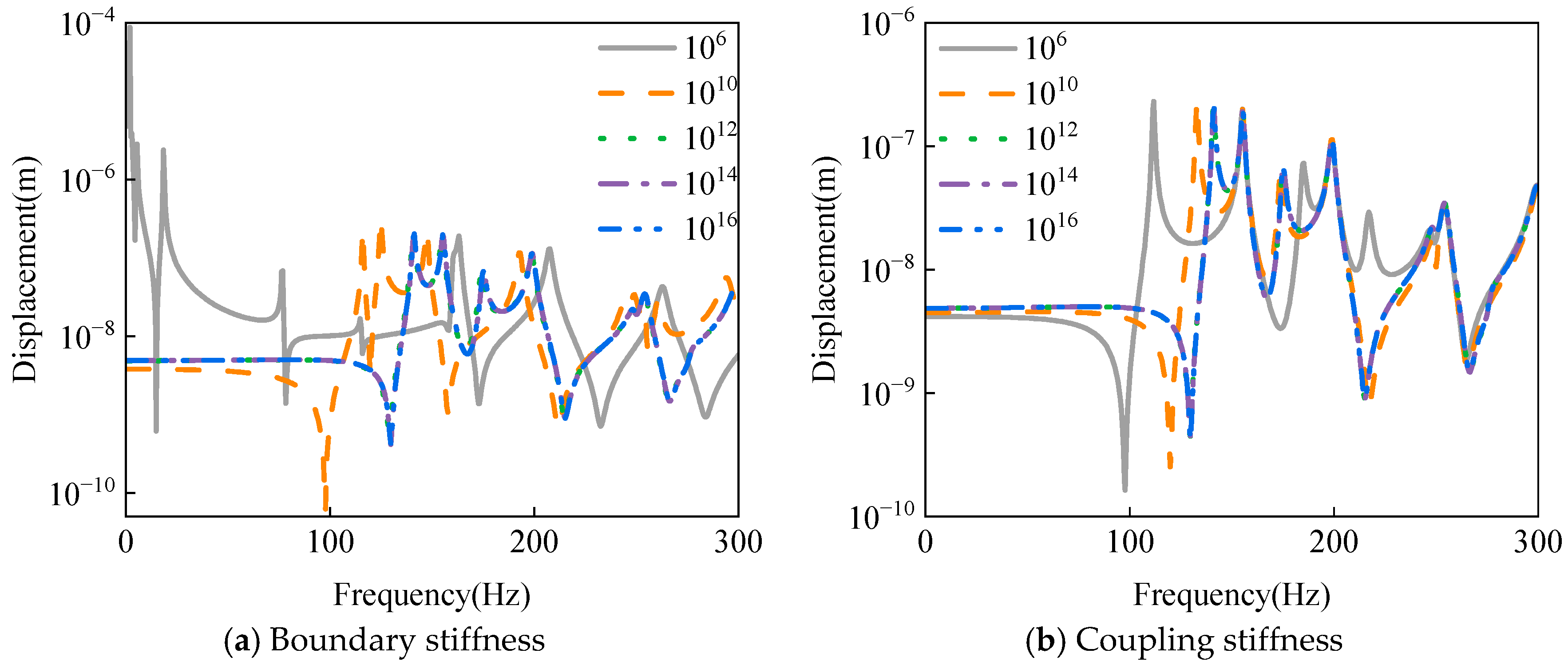
| Boundary Set | ku | kv | kw | kα | kβ |
|---|---|---|---|---|---|
| C (Clamped) | 1014 | 1014 | 1014 | 1014 | 1014 |
| F (Free) | 0 | 0 | 0 | 0 | 0 |
| Mode | Axial Displacement Function Truncation Numbers | Diff. (%) | ||||||
|---|---|---|---|---|---|---|---|---|
| M = 8 | M = 10 | M = 12 | M = 14 | M = 16 | M = 18 | Ref. [44] | ||
| 1 | 49.41 | 49.37 | 49.33 | 49.32 | 49.32 | 49.32 | 49.35 | 0.0608 |
| 2 | 137.43 | 137.31 | 137.20 | 137.17 | 137.17 | 137.17 | 137.2 | 0.0219 |
| 3 | 262.02 | 261.81 | 261.61 | 261.55 | 261.54 | 261.54 | 261.6 | 0.0229 |
| 4 | 364.52 | 364.35 | 364.19 | 364.13 | 364.12 | 364.12 | 363.5 | 0.1706 |
| 5 | 408.23 | 408.17 | 408.11 | 408.09 | 408.08 | 408.08 | 407.9 | 0.0441 |
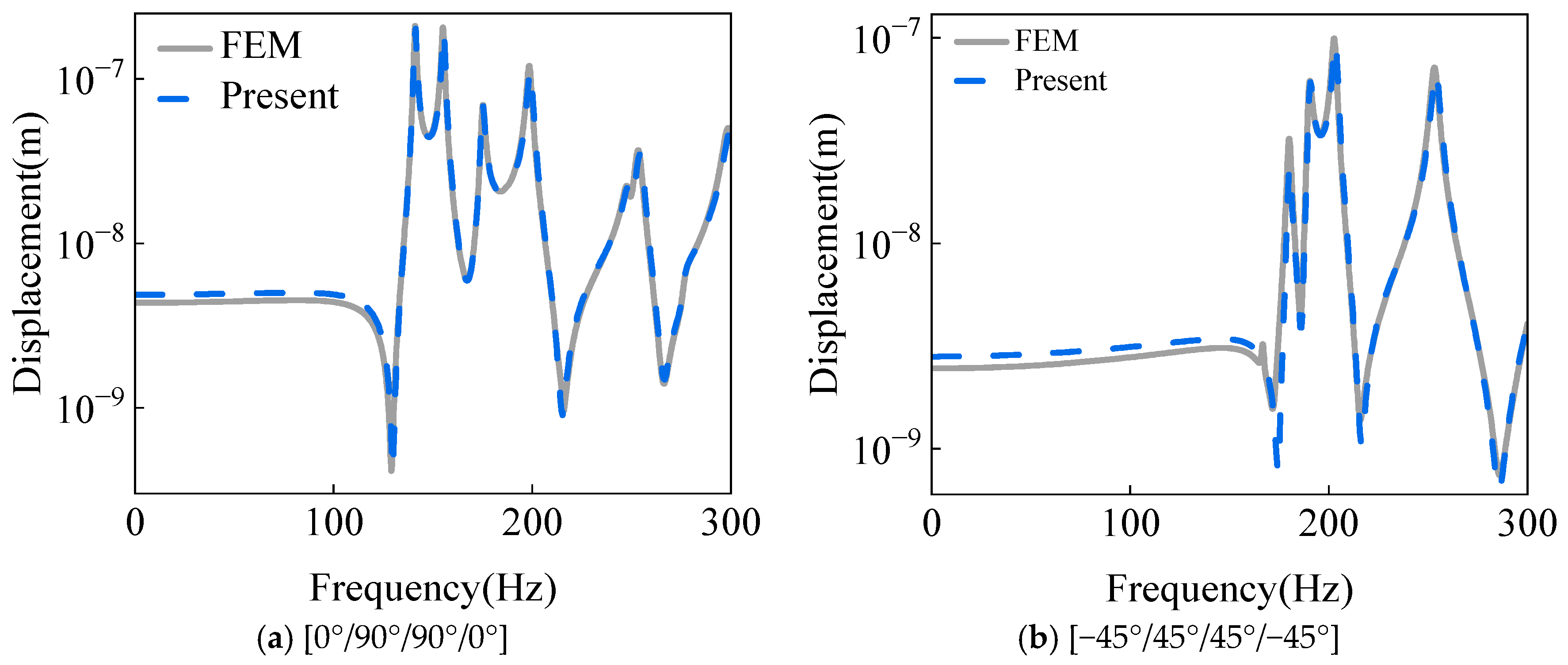
| B.C | Mode | [0°/90°/90°/0°] | [−45°/45°/45°/−45°] | ||||
|---|---|---|---|---|---|---|---|
| Present | FEM | Diff. (%) | Present | FEM | Diff. (%) | ||
| C | 1 | 127.99 | 127.81 | 0.1406 | 167.12 | 166.71 | 0.2453 |
| 3 | 141.05 | 141.00 | 0.0394 | 180.06 | 180.02 | 0.0222 | |
| 5 | 155.44 | 155.10 | 0.2187 | 190.46 | 190.15 | 0.1628 | |
| 7 | 175.05 | 175.06 | 0.0057 | 203.39 | 202.79 | 0.2950 | |
| 9 | 199.08 | 198.54 | 0.2712 | 253.90 | 253.16 | 0.2915 | |
| F | 7 | 17.52 | 17.38 | 0.7991 | 22.80 | 22.23 | 2.5000 |
| 9 | 44.10 | 43.96 | 0.3175 | 51.32 | 50.86 | 0.8963 | |
| 11 | 75.07 | 74.86 | 0.2797 | 85.84 | 85.32 | 0.6058 | |
| 13 | 113.10 | 112.77 | 0.2918 | 128.20 | 127.61 | 0.4602 | |
| 15 | 135.84 | 135.52 | 0.2356 | 146.03 | 145.15 | 0.6026 | |
| Correlation Function | Expression |
|---|---|
| Gaussian | |
| Spline | |
| Matérn (v = 5/2) | |
| Spherical |
| Function | Expression | Dimensions | Range |
|---|---|---|---|
| Michalewicz Function (F1) | 1 | [0, π] | |
| Gramacy & Lee Function (F2) | 1 | [0.5, 2.5] | |
| Rotated Hyper-Ellipsoid Function (F3) | 2 | [−65.536, 65.536] | |
| Three-Hump Camel Function (F4) | 2 | [−5, 5] | |
| Zakharov Function (F5) | 3 | [−5, 10] |
| Function | Correlation Function | ||||||||||||||
|---|---|---|---|---|---|---|---|---|---|---|---|---|---|---|---|
| Gaussian | Spline | Matérn5 | Spherical | AHC-Kriging | Co-Kriging | Stacked-GP | |||||||||
| Average | Variance | Average | Variance | Average | Variance | Average | Variance | Average | Variance | Weight | Average | Variance | Average | Variance | |
| F1 | 0.85 | 5.4 × 10⁻³ | 0.82 | 3.6 × 10⁻² | 0.86 | 1.2 × 10⁻² | 0.82 | 2.8 × 10⁻² | 0.87 | 5.6 × 10⁻³ | 0.875 | 0.82 | 1.0 × 10⁻² | 0.84 | 2.4 × 10⁻² |
| F2 | 0.87 | 1.2 × 10⁻³ | 0.88 | 9.1 × 10⁻⁴ | 0.88 | 9.1 × 10⁻⁴ | 0.87 | 1.2 × 10⁻³ | 0.89 | 6.9 × 10⁻⁴ | 0.026 | 0.88 | 7.3 × 10⁻⁴ | 0.93 | 5.2 × 10⁻³ |
| F3 | 1 | 2.4 × 10⁻²⁰ | 0.98 | 2.5 × 10⁻⁶ | 1 | 3.9 × 10⁻¹⁷ | 0.92 | 5.7 × 10⁻⁴ | 1 | 1.7 × 10⁻¹⁰ | 0.116 | 1 | 7.5 × 10⁻¹⁴ | 1 | 5.9 × 10⁻⁸ |
| F4 | 1 | 4.7 × 10⁻⁶ | 0.99 | 8.4 × 10⁻⁶ | 1 | 2.0 × 10⁻⁶ | 0.95 | 1.2 × 10⁻³ | 1 | 4.8 × 10⁻⁷ | 0.416 | 0.98 | 4.5 × 10⁻⁴ | 0.93 | 4.9 × 10⁻² |
| F5 | 0.96 | 8.3 × 10⁻³ | 0.80 | 1.1 × 10⁻¹ | 0.93 | 1.6 × 10⁻² | 0.77 | 2.7 × 10⁻² | 0.97 | 1.0 × 10⁻³ | 0.473 | 0.95 | 4.9 × 10⁻³ | 0.95 | 2.5 × 10⁻³ |
| Function | Correlation Function | ||||||||||||||
|---|---|---|---|---|---|---|---|---|---|---|---|---|---|---|---|
| Gaussian | Spline | Matérn5 | Spherical | AHC-Kriging | Co-Kriging | Stacked-GP | |||||||||
| Average | Variance | Average | Variance | Average | Variance | Average | Variance | Average | Variance | Weight | Average | Variance | Average | Variance | |
| F1 | 0.081 | 3.8 × 10⁻⁴ | 0.082 | 1.6 × 10⁻³ | 0.075 | 9.0 × 10⁻⁴ | 0.085 | 1.3 × 10⁻³ | 0.077 | 4.4 × 10⁻⁴ | 0.875 | 0.089 | 7.3 × 10⁻⁴ | 0.078 | 1.5 × 10⁻³ |
| F2 | 0.460 | 3.6 × 10⁻³ | 0.448 | 3.0 × 10⁻³ | 0.449 | 3.0 × 10⁻³ | 0.459 | 4.0 × 10⁻³ | 0.443 | 2.4 × 10⁻³ | 0.026 | 0.457 | 2.5 × 10⁻³ | 0.389 | 2.5 × 10⁻² |
| F3 | 0.028 | 2.8 × 10⁻⁴ | 120.1 | 2.5 × 10³ | 0.282 | 7.9 × 10⁻³ | 825.5 | 1.4 × 10⁴ | 0.322 | 3.5 × 10⁻³ | 0.116 | 0.487 | 6.2 × 10⁻¹ | 0.840 | 6.2 × 10⁻¹ |
| F4 | 25.93 | 71.41 | 33.28 | 79.93 | 25.34 | 37.56 | 87.82 | 1.3 × 10⁴ | 24.62 | 9.974 | 0.416 | 57.08 | 938.9 | 54.50 | 1.4 × 10⁴ |
| F5 | 1.3 × 10⁴ | 7.8 × 10⁷ | 2.7 × 10⁴ | 3.7 × 10⁸ | 1.8 × 10⁴ | 8.9 × 10⁷ | 3.5 × 10⁴ | 1.2 × 10⁸ | 1.3 × 10⁴ | 3.0 × 10⁷ | 0.473 | 1.3 × 10⁴ | 1.1 × 10⁶ | 1.4 × 10⁴ | 4.5 × 10⁷ |
| Variables | Range |
|---|---|
| E1/GPa | [142.5, 157.5] |
| E2/GPa | [9.5, 10.5] |
| μ12 | [0.2375, 0.2625] |
| G12/GPa | [5.7, 6.3] |
| G13/GPa | [5.7, 6.3] |
| G23/GPa | [4.75, 5.25] |
| ρ/kg·m−3 | [1377.5, 1522.5] |
| Surrogate | 14 | 35 | 70 | 105 | 140 | 175 |
|---|---|---|---|---|---|---|
| Average | Average | Average | Average | Average | Average | |
| Kriging–Gaussian | 0.969 | 0.989 | 0.993 | 0.996 | 0.997 | 0.998 |
| Kriging–spline | 0.935 | 0.982 | 0.996 | 0.996 | 0.997 | 0.998 |
| Kriging–Matérn5 | 0.972 | 0.989 | 0.996 | 0.996 | 0.997 | 0.998 |
| Kriging–spherical | 0.958 | 0.987 | 0.992 | 0.993 | 0.994 | 0.996 |
| Co-Kriging | 0.931 | 0.989 | 0.996 | 0.996 | 0.997 | 0.997 |
| Stacked-GP | 0.766 | 0.792 | 0.816 | 0.831 | 0.851 | 0.875 |
| Surrogate | 14 | 35 | 70 | 105 | 140 | 175 |
|---|---|---|---|---|---|---|
| Average | Average | Average | Average | Average | Average | |
| Kriging–Gaussian | 4.7859 × 10⁻⁹ | 2.9287 × 10⁻⁹ | 2.2708 × 10⁻⁹ | 1.9247 × 10⁻⁹ | 1.7091 × 10⁻⁹ | 1.3201 × 10⁻⁹ |
| Kriging–spline | 6.1931 × 10⁻⁹ | 3.3125 × 10⁻⁹ | 1.9922 × 10⁻⁹ | 1.9353 × 10⁻⁹ | 1.5768 × 10⁻⁹ | 1.3777 × 10⁻⁹ |
| Kriging-Matérn5 | 4.5482 × 10⁻⁹ | 2.9493 × 10⁻⁹ | 2.0432 × 10⁻⁹ | 1.9351 × 10⁻⁹ | 1.5244 × 10⁻⁹ | 1.3934 × 10⁻⁹ |
| Kriging–spherical | 5.0981 × 10⁻⁹ | 3.4330 × 10⁻⁹ | 2.8111 × 10⁻⁹ | 2.6229 × 10⁻⁹ | 2.2172 × 10⁻⁹ | 2.0798 × 10⁻⁹ |
| Co-Kriging | 5.7623 × 10⁻⁹ | 2.9657 × 10⁻⁹ | 2.0749 × 10⁻⁹ | 1.9890 × 10⁻⁹ | 1.6152 × 10⁻⁹ | 1.4120 × 10⁻⁹ |
| Stacked-GP | 9.4869 × 10⁻⁹ | 9.2354 × 10⁻⁹ | 9.1748 × 10⁻⁹ | 8.3178 × 10⁻⁹ | 8.1108 × 10⁻⁹ | 7.6898 × 10⁻⁹ |
| Hybrid Correlation Function | Weight | Average of Q2 | Average of RSME | Variance of Q2 | Variance of RSME |
|---|---|---|---|---|---|
| Gaussian + Spline | 0.9299 | 0.997 | 1.8620 × 10⁻⁹ | 8.8759 × 10⁻⁷ | 3.3626 × 10⁻²⁰ |
| Gaussian + Matérn5 | 0.2720 | 0.997 | 1.7844 × 10⁻⁹ | 1.7453 × 10⁻⁷ | 9.1235 × 10⁻²¹ |
| Spline + Matérn5 | 0.1868 | 0.998 | 1.6975 × 10⁻⁹ | 2.4369 × 10⁻⁸ | 1.8450 × 10⁻²¹ |
| Test Functions | Expression | Dimensions | Range |
|---|---|---|---|
| ZDT1 | 30 | [0, 1] | |
| ZDT2 | 30 | [0, 1] | |
| ZDT3 | 30 | [0, 1] | |
| Kursawe | 3 | [−5, 5] |
| Test Functions | Indicators | IMSSA | MSSA | NSGA-II | MOPSO |
|---|---|---|---|---|---|
| ZDT1 | Average | 0.0020 | 0.0095 | 0.0356 | 0.0354 |
| Std. | 7.727 × 10⁻⁷ | 2.284 × 10⁻⁶ | 2.856 × 10⁻⁵ | 2.739 × 10⁻⁶ | |
| ZDT2 | Average | 0.0032 | 0.0135 | 0.0391 | 0.0326 |
| Std. | 7.676 × 10⁻⁶ | 8.294 × 10⁻⁶ | 2.886 × 10⁻⁴ | 8.191 × 10⁻⁶ | |
| ZDT3 | Average | 0.0053 | 0.0107 | 0.0316 | 0.0131 |
| Std. | 1.648 × 10⁻⁵ | 4.546 × 10⁻⁵ | 2.403 × 10⁻⁵ | 7.329 × 10⁻⁶ | |
| Kursawe | Average | 0.0106 | 0.0316 | 0.0070 | 0.0392 |
| Std. | 1.733 × 10⁻⁵ | 2.347 × 10⁻⁴ | 2.262 × 10⁻⁶ | 6.863 × 10⁻⁴ |
| Test Functions | Indicators | IMSSA | MSSA | NSGA-II | MOPSO |
|---|---|---|---|---|---|
| ZDT1 | Average | 0.6767 | 0.5368 | 0.3818 | 0.3652 |
| Std. | 9.819 × 10⁻⁶ | 2.341 × 10⁻⁴ | 0.0016 | 4.923 × 10⁻⁵ | |
| ZDT2 | Average | 0.3918 | 0.1905 | 0.1334 | 0.1073 |
| Std. | 1.189 × 10⁻⁴ | 2.978 × 10⁻⁴ | 1.747 × 10⁻⁴ | 1.450 × 10⁻⁶ | |
| ZDT3 | Average | 0.6116 | 0.5184 | 0.3922 | 0.6012 |
| Std. | 7.648 × 10⁻⁴ | 0.0049 | 0.0021 | 9.840 × 10⁻⁴ | |
| Kursawe | Average | 0.5085 | 0.4986 | 0.5010 | 0.5899 |
| Std. | 0.0027 | 0.0036 | 2.857 × 10⁻⁵ | 0.0063 |
| Surrogate | Average of Q2 | Average of RMSE | Variance of Q2 | Variance of RMSE |
|---|---|---|---|---|
| Kriging–Gaussian | 0.8495 | 5.6457 × 10⁻² | 4.0534 × 10⁻² | 6.9082 × 10⁻⁴ |
| Kriging–spline | 0.5568 | 9.2001 × 10⁻² | 1.9463 × 10⁻¹ | 2.9661 × 10⁻³ |
| Kriging–Matérn5 | 0.8873 | 5.1816 × 10⁻² | 2.7555 × 10⁻² | 4.7375 × 10⁻⁴ |
| Kriging–spherical | 0.9244 | 4.4087 × 10⁻² | 2.0621 × 10⁻⁶ | 1.7236 × 10⁻⁷ |
| AHC-Kriging | 0.9255 | 4.3748 × 10⁻² | 1.5420 × 10⁻⁵ | 1.3326 × 10⁻⁶ |
| Co-Kriging | 0.8664 | 1.2103 × 10⁻¹ | 1.2738 × 10⁻³ | 2.7781 × 10⁻³ |
| Stacked-GP | 0.8266 | 2.1796 × 10⁻¹ | 3.5762 × 10⁻² | 4.2334 × 10⁻² |
| Surrogate | Average of Q2 | Average of RMSE | Variance of Q2 | Variance of RMSE |
|---|---|---|---|---|
| Kriging–Gaussian | 0.8528 | 4.5773 | 8.4366 × 10⁻² | 14.774 |
| Kriging–spline | 0.3468 | 11.172 | 1.9722 × 10⁻¹ | 33.313 |
| Kriging–Matérn5 | 0.7771 | 5.6911 | 1.1666 × 10⁻¹ | 21.694 |
| Kriging–spherical | 0.7522 | 6.4808 | 1.2180 × 10⁻¹ | 18.046 |
| AHC-Kriging | 0.9238 | 4.0970 | 5.0279 × 10⁻³ | 1.6290 |
| Co-Kriging | 0.8198 | 5.6620 | 8.7001 × 10⁻² | 12.716 |
| Stacked-GP | 0.8263 | 5.3319 | 7.2392 × 10⁻² | 14.998 |
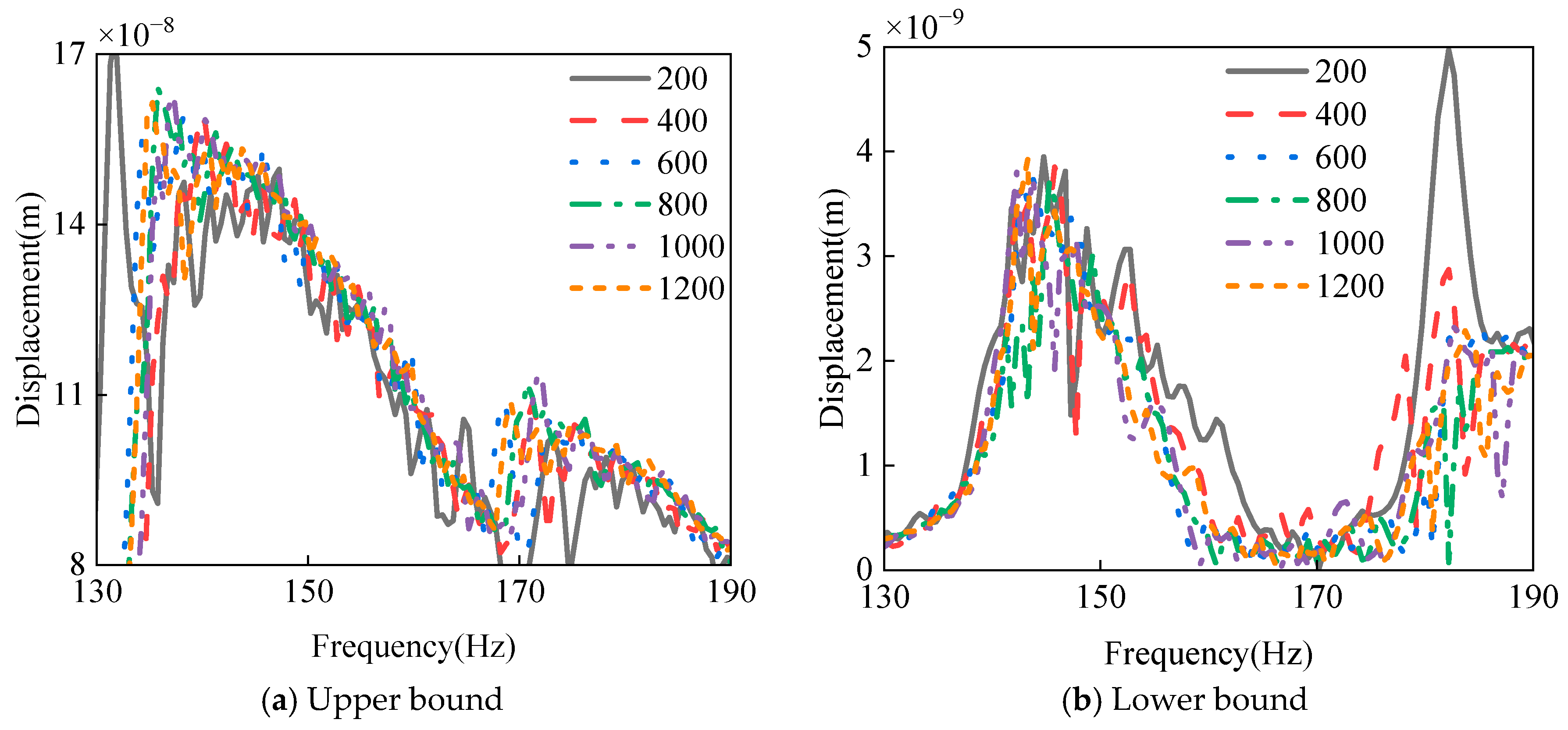
| Obj. | 200 | 400 | 600 | 800 | 1000 | 1200 |
|---|---|---|---|---|---|---|
| Dc | 8.9219 × 10⁻⁸ | 8.1390 × 10⁻⁸ | 8.1565 × 10⁻⁸ | 8.3844 × 10⁻⁸ | 8.3287 × 10⁻⁸ | 8.3194 × 10⁻⁸ |
| Dw | 8.4250 × 10⁻⁸ | 7.7539 × 10⁻⁸ | 7.7828 × 10⁻⁸ | 7.9828 × 10⁻⁸ | 7.9486 × 10⁻⁸ | 7.9266 × 10⁻⁸ |
| Fc | 132.3364 | 133.3849 | 132.5577 | 132.3604 | 131.8038 | 131.8683 |
| Fw | 13.0238 | 15.3907 | 15.5161 | 16.0973 | 15.9519 | 15.8611 |
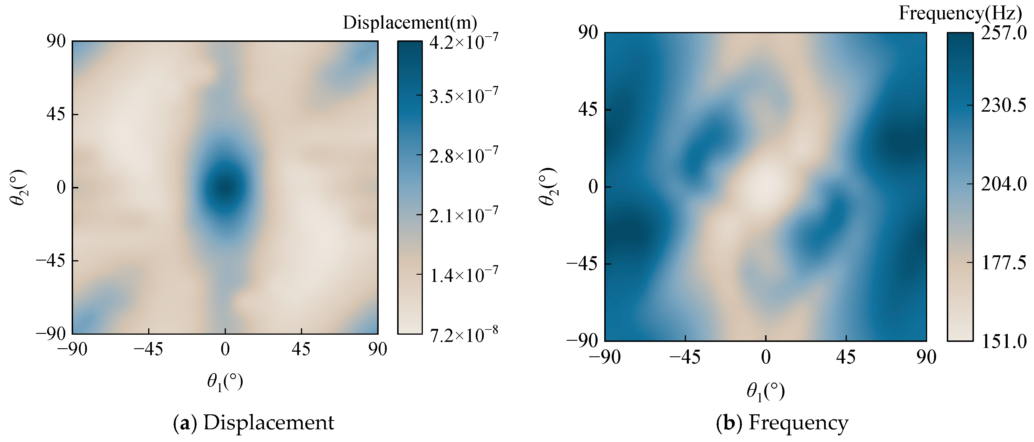
| Case | θ1/° | θ2/° | Dc (×10−8 m) | Diff.(%) | Dw (×10−8 m) | Diff.(%) | Fc(Hz) | Diff. (%) | Fw (Hz) | Diff. (%) |
|---|---|---|---|---|---|---|---|---|---|---|
| 1 (Original) | 0 | 90 | 8.3287 | —— | 7.9486 | —— | 131.8038 | —— | 15.9519 | —— |
| 2 (min Dc) | 51.45 | −34.13 | 3.4501 | 58.58 | 3.1316 | 60.60 | 175.4543 | 33.1178 | 21.7264 | 36.1994 |
| 3 (max Fc) | 50.48 | −18.03 | 3.5248 | 57.68 | 3.3083 | 58.38 | 178.2618 | 35.2478 | 19.8576 | 24.4842 |
| 4 (min Fw) | −90 | −90 | 10.0058 | 20.14 | 8.8292 | 11.08 | 119.1401 | 9.6080 | 6.1280 | 61.5845 |
Disclaimer/Publisher’s Note: The statements, opinions and data contained in all publications are solely those of the individual author(s) and contributor(s) and not of MDPI and/or the editor(s). MDPI and/or the editor(s) disclaim responsibility for any injury to people or property resulting from any ideas, methods, instructions or products referred to in the content. |
© 2025 by the authors. Licensee MDPI, Basel, Switzerland. This article is an open access article distributed under the terms and conditions of the Creative Commons Attribution (CC BY) license (https://creativecommons.org/licenses/by/4.0/).
Share and Cite
Huang, T.; Wang, Q.; Zhong, R.; Liu, T. An Adaptive Hybrid Correlation Kriging Approach for Uncertainty Dynamic Optimization of Spherical-Conical Shell Structure. Materials 2025, 18, 3588. https://doi.org/10.3390/ma18153588
Huang T, Wang Q, Zhong R, Liu T. An Adaptive Hybrid Correlation Kriging Approach for Uncertainty Dynamic Optimization of Spherical-Conical Shell Structure. Materials. 2025; 18(15):3588. https://doi.org/10.3390/ma18153588
Chicago/Turabian StyleHuang, Tianchen, Qingshan Wang, Rui Zhong, and Tao Liu. 2025. "An Adaptive Hybrid Correlation Kriging Approach for Uncertainty Dynamic Optimization of Spherical-Conical Shell Structure" Materials 18, no. 15: 3588. https://doi.org/10.3390/ma18153588
APA StyleHuang, T., Wang, Q., Zhong, R., & Liu, T. (2025). An Adaptive Hybrid Correlation Kriging Approach for Uncertainty Dynamic Optimization of Spherical-Conical Shell Structure. Materials, 18(15), 3588. https://doi.org/10.3390/ma18153588