Prediction of Failure Pressure of Sulfur-Corrosion-Defective Pipelines Based on GABP Neural Networks


Abstract
1. Introduction
2. The Effect of Sulfur-Containing Corrosion on the Performance of Pipeline Materials
2.1. Materials and Methods
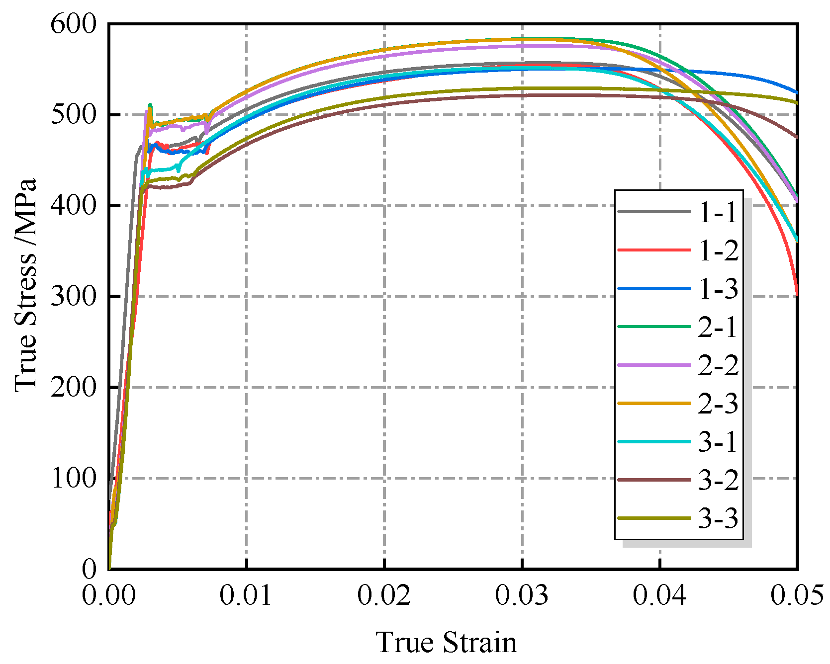
2.2. Test Results and Analysis
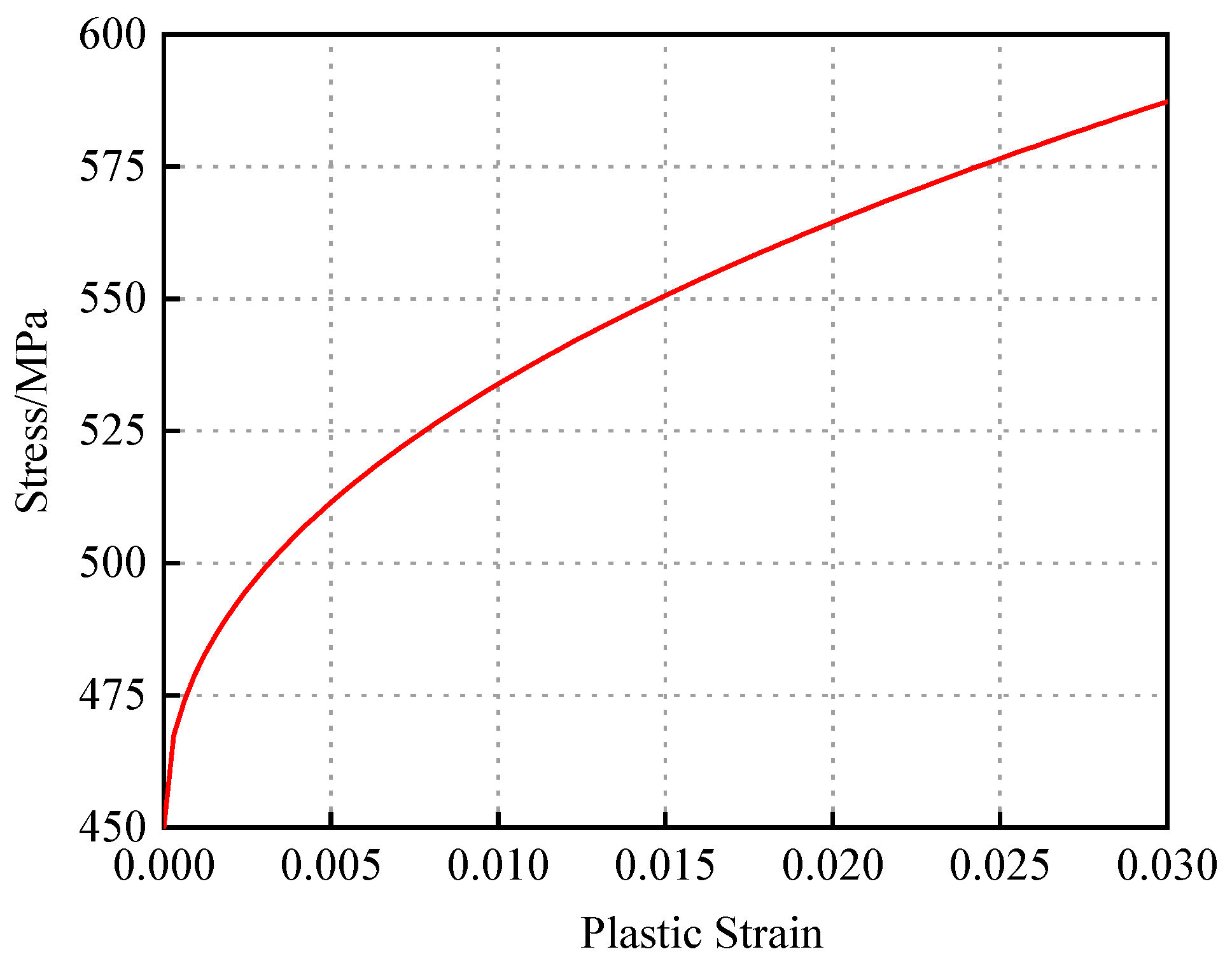
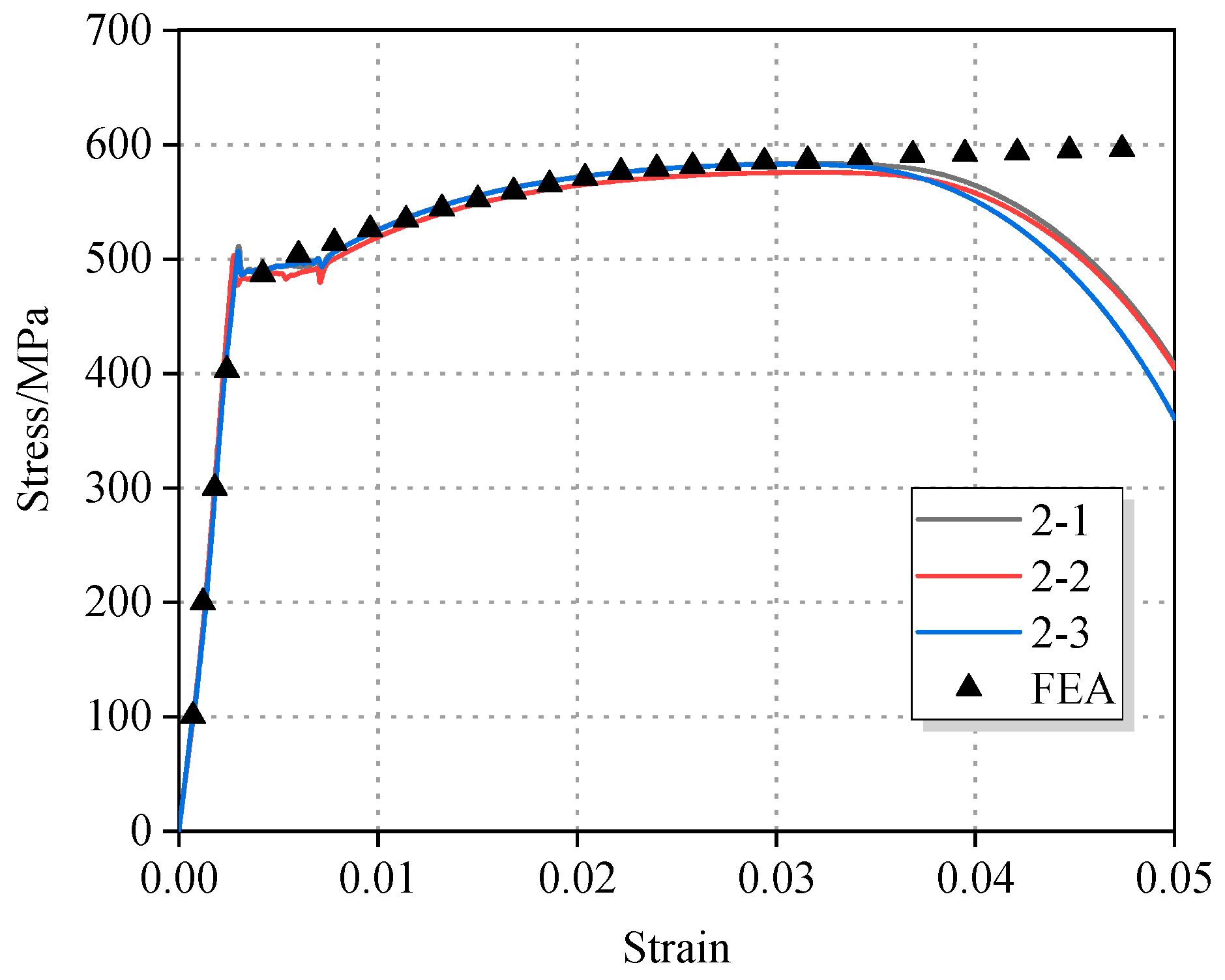
2.3. Constitutive Model
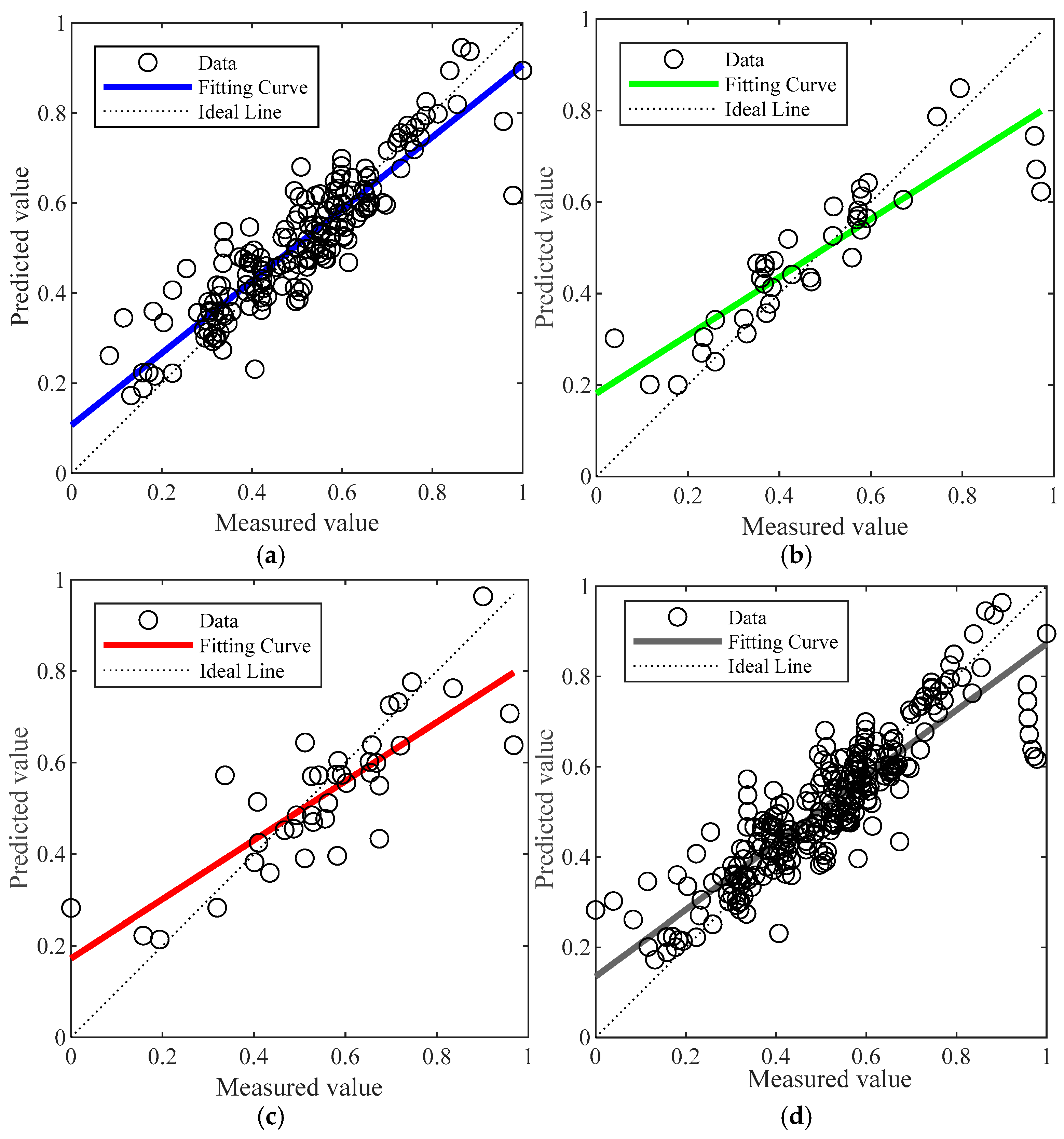
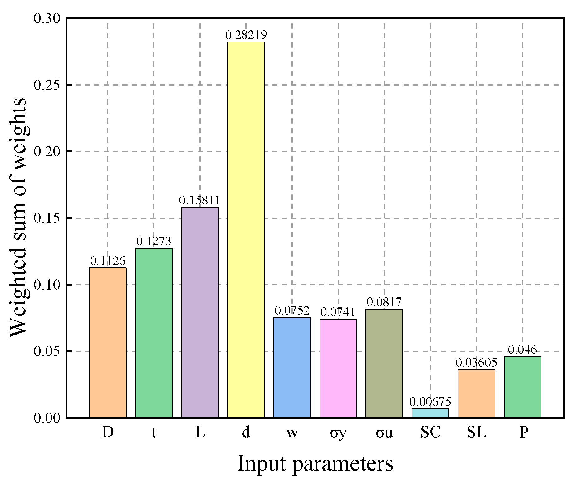
3. Prediction of Failure Pressure
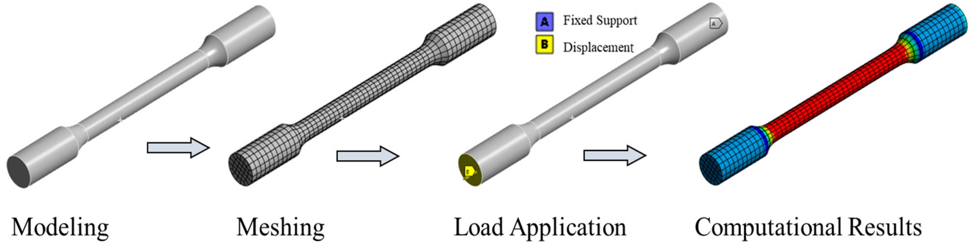
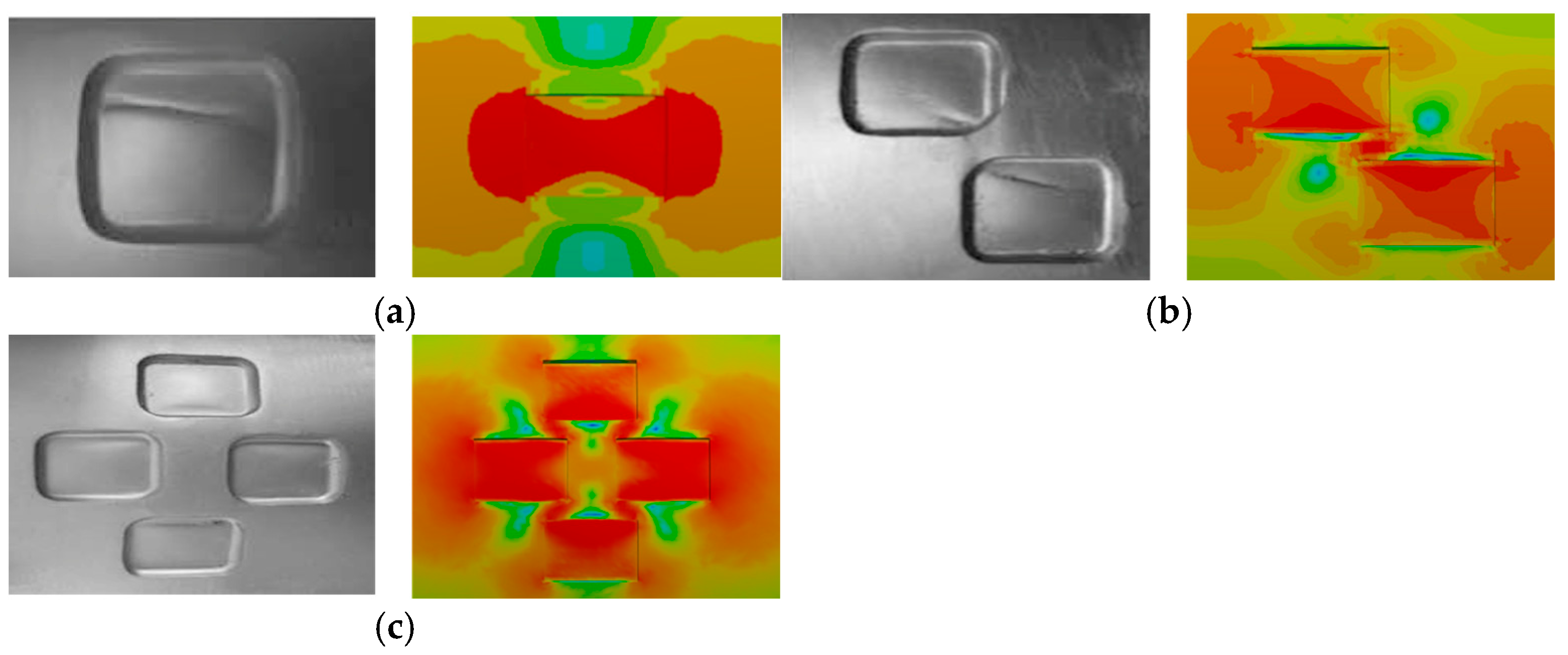
3.1. Finite Element Model
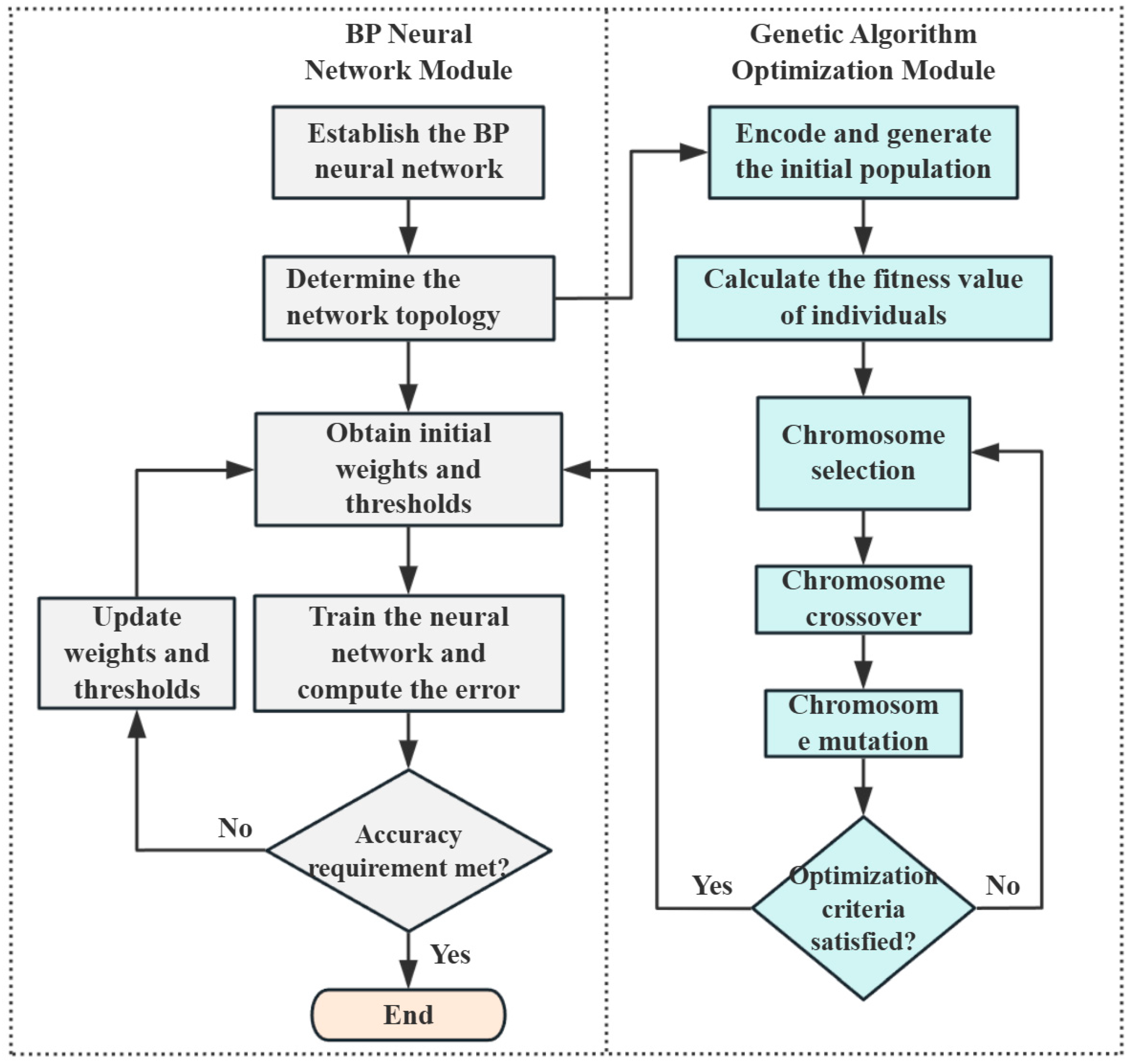
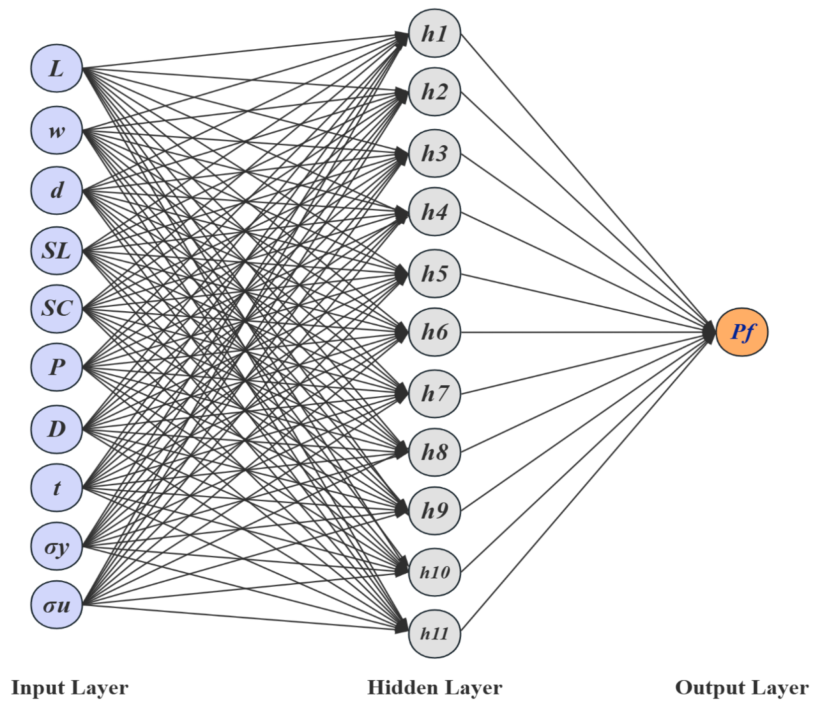
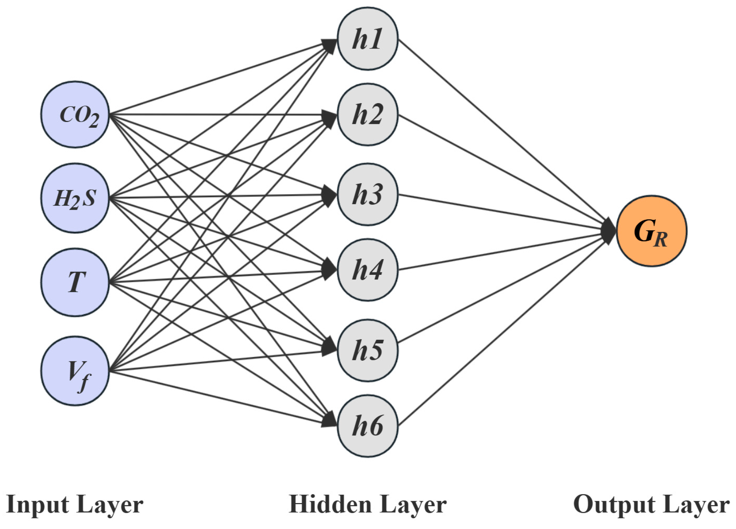
3.2. GABP Neural Network Model
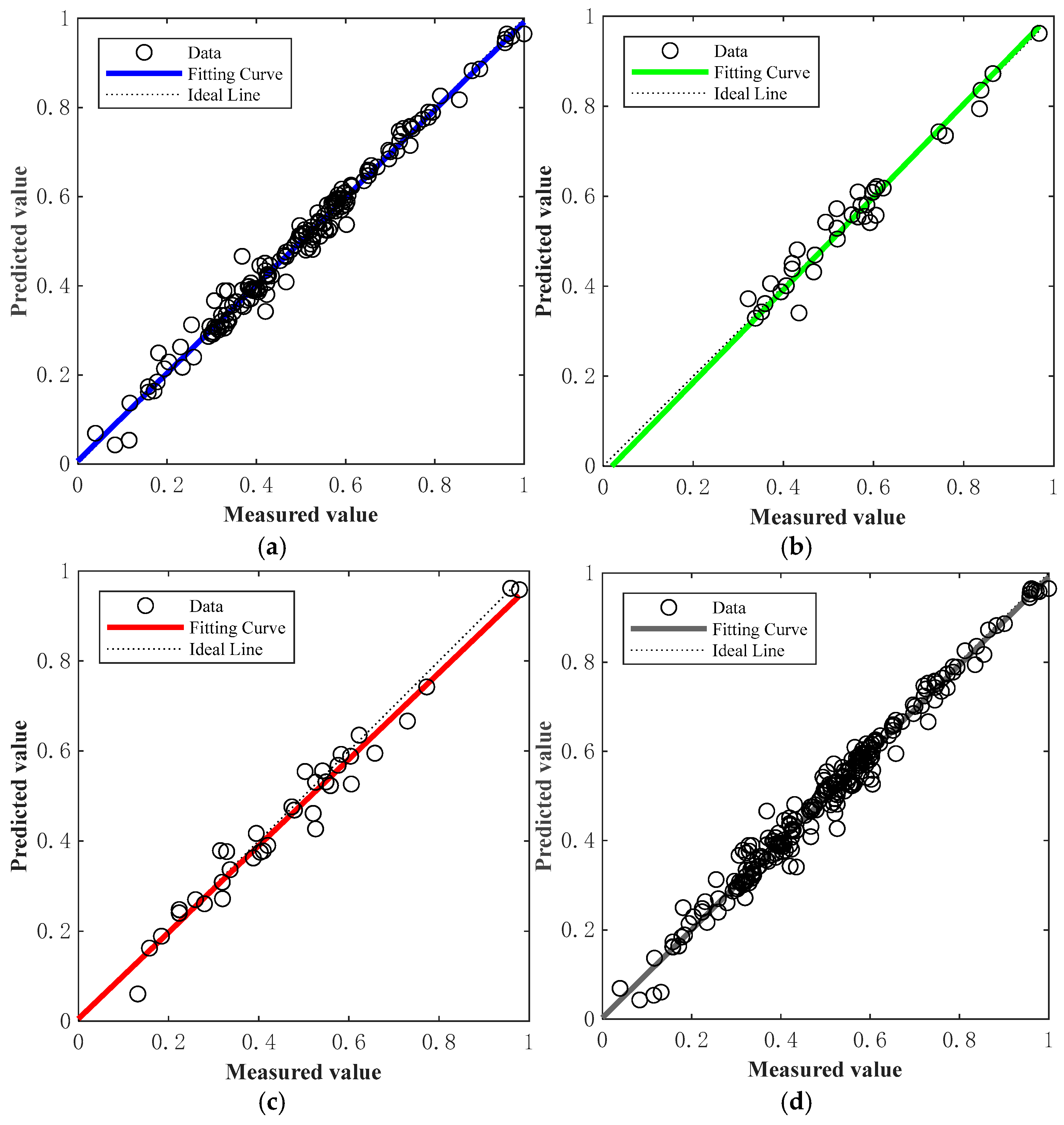
3.3. Optimized Results
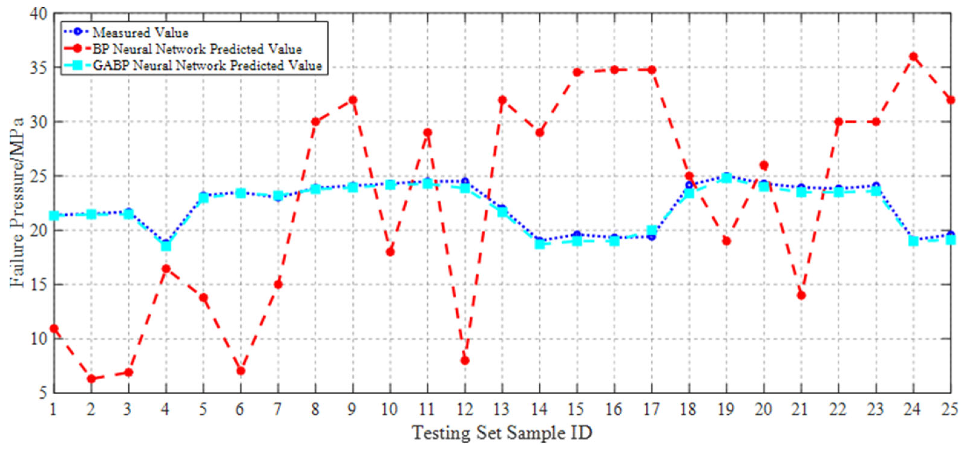
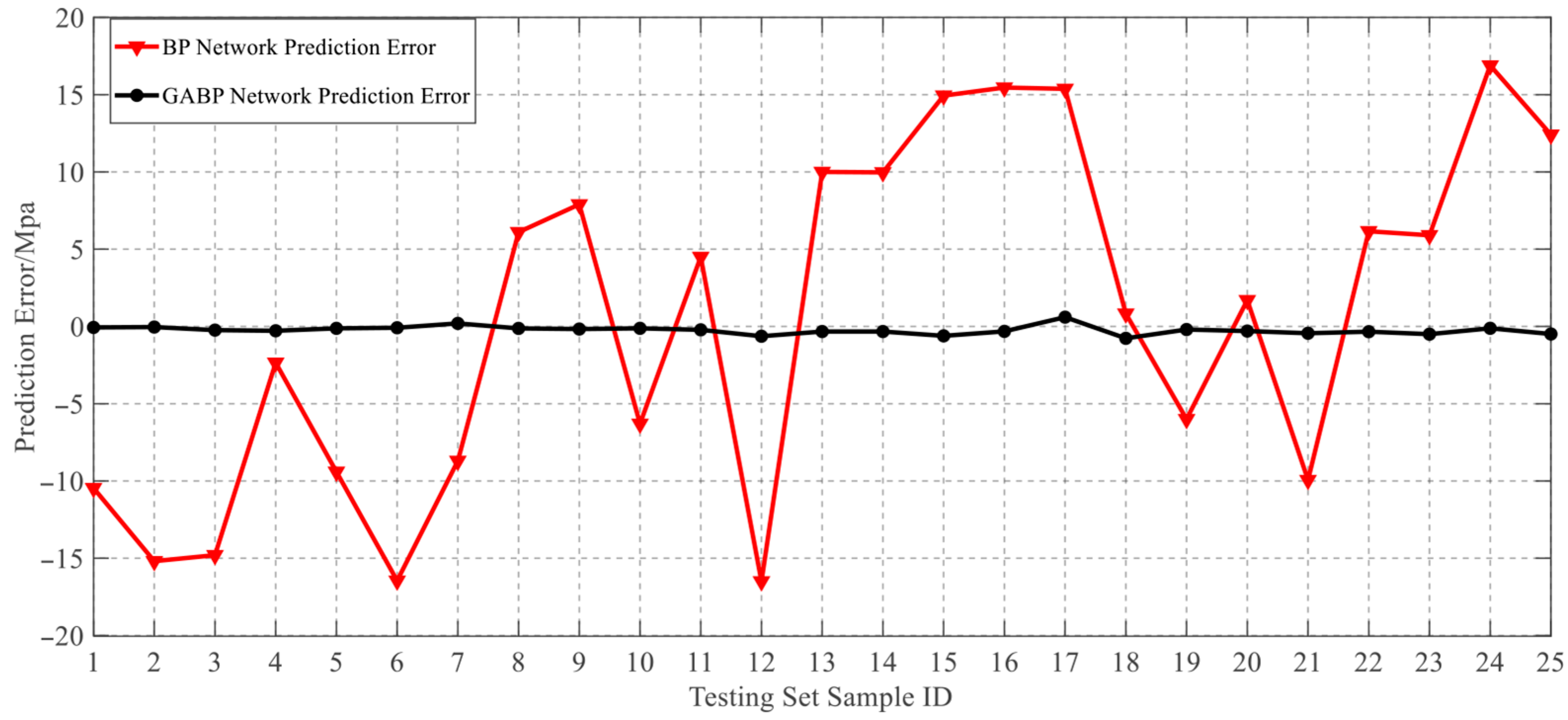
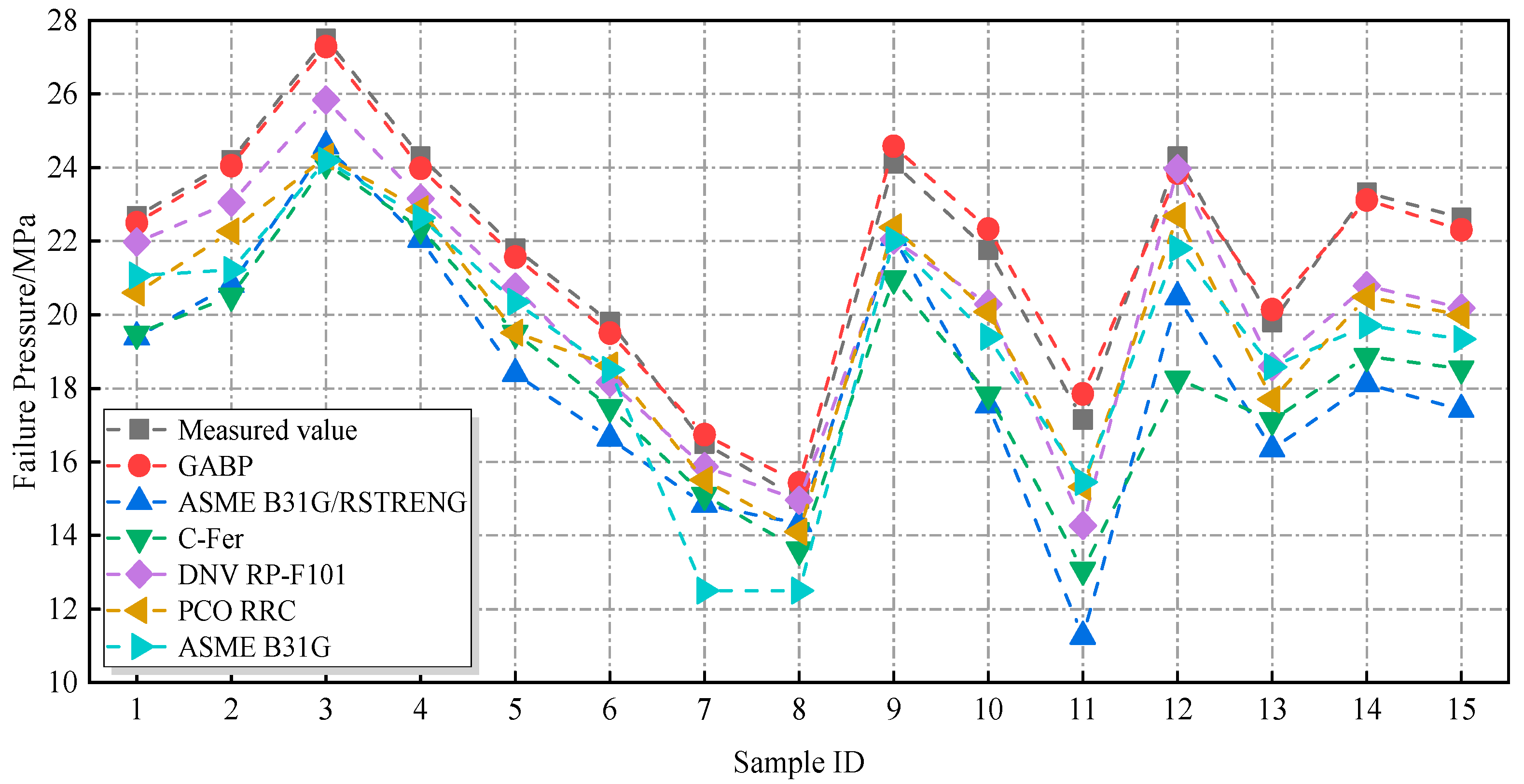
3.4. Model Validation
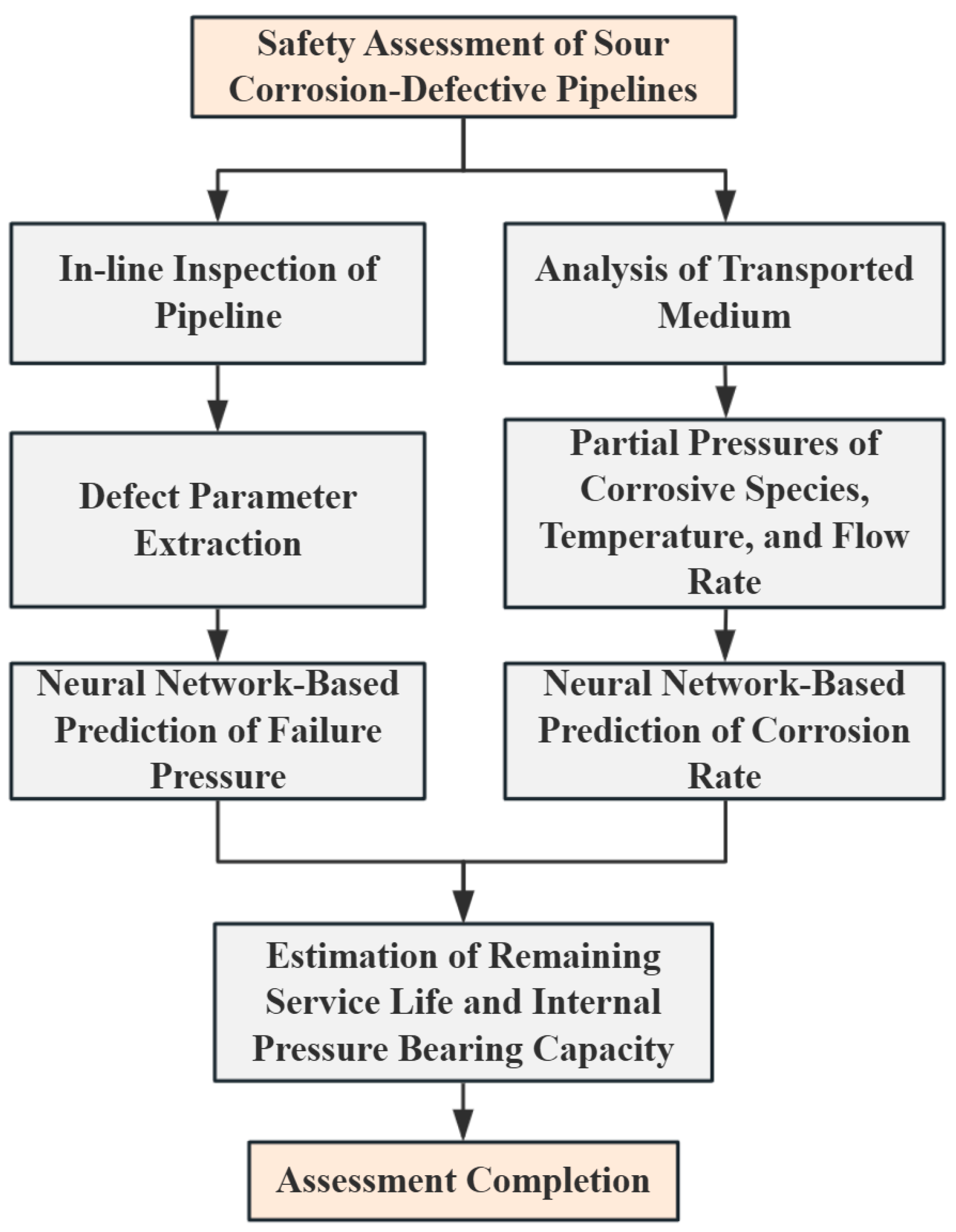
4. Prediction of Remaining Life of Pipelines
4.1. Corrosion Rate Prediction Model
4.2. Remaining Life Prediction Method
4.3. Model Application Illustrative Example
5. Conclusions
- (1)
- The mechanical properties of pipeline steel exposed to high-sulfur corrosive environments were experimentally investigated to assess the effects of such harsh service conditions on material strength degradation. The results indicated that, despite prolonged exposure to a high-sulfur environment, the material property parameters of the corroded pipeline steel exhibited no significant degradation in its intrinsic mechanical properties, although geometric stability was reduced due to corrosion.
- (2)
- The Johnson–Cook constitutive model for X52 pipeline steel was calibrated, with the numerical simulation results showing a high degree of agreement with the experimental curves. This constitutive model was demonstrated to accurately describe the plastic hardening characteristics of X52 steel.
- (3)
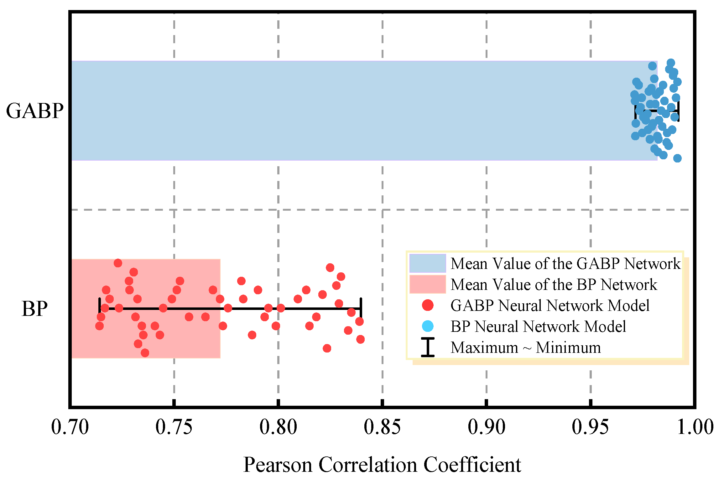
- A genetic algorithm-optimized backpropagation (GABP) neural network model was developed to predict the failure pressure and corrosion rate of defected pipelines. The predictive accuracy and fitting performance of the GABP model were compared with those of the conventional BP neural network. The results show that the GABP neural network achieved higher prediction accuracy for both the pipeline failure pressure and X52 sulfur corrosion rate, with maximum errors of 4.08% and 7.94%, respectively. Furthermore, based on the two neural network models, the failure pressure and service life of an in-service pipeline in a sulfur-containing gas field were predicted, demonstrating strong practical engineering guidance value.
Author Contributions
Funding
Institutional Review Board Statement
Informed Consent Statement
Data Availability Statement
Conflicts of Interest
Appendix A

| Serial Number | D/mm | t/mm | L/mm | d/mm | w/mm | Material | σy/MPa | σu/MPa | Pf/MPa |
|---|---|---|---|---|---|---|---|---|---|
| 1 | 458.8 | 8.10 | 39.60 | 5.39 | 31.90 | X80 | 601.00 | 684.00 | 22.68 |
| 2 | 459.4 | 8.00 | 40.05 | 3.75 | 32.00 | X80 | 589.00 | 730.50 | 24.20 |
| 3 | 762 | 17.50 | 50.00 | 8.75 | 50.00 | X52 | 495.00 | 565.00 | 27.50 |
| 4 | 762 | 17.50 | 100.00 | 8.75 | 50.00 | X52 | 495.00 | 565.00 | 24.30 |
| 5 | 762 | 17.50 | 200.00 | 8.75 | 50.00 | X52 | 495.00 | 565.00 | 21.80 |
| 6 | 762 | 17.50 | 300.00 | 8.75 | 50.00 | X52 | 495.00 | 565.00 | 19.80 |
| 7 | 762 | 17.50 | 600.00 | 8.75 | 50.00 | X52 | 495.00 | 565.00 | 16.50 |
| 8 | 762 | 17.50 | 900.00 | 8.75 | 50.00 | X52 | 495.00 | 565.00 | 15.00 |
| 9 | 762 | 17.50 | 200.00 | 4.20 | 50.00 | X52 | 474.10 | 556.60 | 24.11 |
| 10 | 762 | 17.50 | 200.00 | 8.90 | 50.00 | X52 | 474.10 | 556.60 | 21.76 |
| 11 | 762 | 17.50 | 200.00 | 13.10 | 50.00 | X52 | 474.10 | 556.60 | 17.15 |
| 12 | 762 | 17.50 | 100.00 | 8.40 | 50.00 | X52 | 474.10 | 556.60 | 24.30 |
| 13 | 762 | 17.50 | 300.00 | 8.50 | 50.00 | X52 | 474.10 | 556.60 | 19.80 |
| 14 | 762 | 17.50 | 200.00 | 8.40 | 100.00 | X52 | 474.10 | 556.60 | 23.42 |
| 15 | 762 | 17.50 | 200.00 | 9.00 | 200.00 | X52 | 474.10 | 556.60 | 22.64 |
| 25 | 1422.4 | 19.25 | 180.00 | 10.40 | 0.50 | X100 | 740.00 | 774.00 | 15.35 |
| 26 | 1422.4 | 20.10 | 385.00 | 3.80 | 0.50 | X100 | 795.00 | 840.00 | 20.12 |
| 27 | 914.4 | 16.40 | 150.00 | 9.00 | 0.50 | X100 | 739.00 | 813.00 | 21.40 |
| 28 | 914.4 | 16.40 | 450.00 | 6.00 | 0.50 | X100 | 739.00 | 813.00 | 24.02 |
| 29 | 324 | 6.40 | 20.70 | 3.23 | 19.30 | X52 | 382.00 | 570.00 | 16.64 |
| 30 | 324 | 6.01 | 19.35 | 3.60 | 18.99 | X52 | 382.00 | 570.00 | 16.22 |
| 31 | 324 | 6.30 | 19.80 | 3.57 | 19.31 | X52 | 373.00 | 522.00 | 15.95 |
| 32 | 324 | 6.31 | 20.13 | 3.73 | 19.74 | X52 | 373.00 | 522.00 | 14.16 |
| 33 | 324 | 6.16 | 20.12 | 3.73 | 19.99 | X52 | 356.00 | 514.00 | 18.85 |
| 34 | 324 | 6.27 | 19.91 | 3.73 | 20.20 | X52 | 356.00 | 514.00 | 19.13 |
| 35 | 324 | 6.25 | 19.93 | 3.76 | 20.11 | X52 | 356.00 | 514.00 | 19.27 |
| 36 | 324 | 6.18 | 19.92 | 3.79 | 20.01 | X52 | 421.00 | 520.00 | 19.44 |
| 37 | 508 | 7.10 | 40.00 | 1.07 | 15.95 | X70 | 485.00 | 590.00 | 19.02 |
| 38 | 508 | 8.70 | 80.00 | 2.61 | 31.90 | X70 | 485.00 | 590.00 | 20.78 |
| 39 | 508 | 10.00 | 150.00 | 4.50 | 47.85 | X70 | 485.00 | 590.00 | 19.54 |
| 40 | 508 | 12.00 | 300.00 | 7.20 | 63.80 | X70 | 485.00 | 590.00 | 16.36 |
| 41 | 508 | 17.50 | 600.00 | 13.13 | 79.76 | X70 | 485.00 | 590.00 | 13.79 |
| 42 | 660 | 7.10 | 80.00 | 3.20 | 82.90 | X70 | 485.00 | 590.00 | 11.75 |
| 43 | 660 | 8.70 | 150.00 | 5.22 | 207.24 | X70 | 485.00 | 590.00 | 11.13 |
| 44 | 660 | 10.00 | 300.00 | 7.50 | 20.72 | X70 | 485.00 | 590.00 | 7.55 |
| 45 | 660 | 12.00 | 600.00 | 1.80 | 41.45 | X70 | 485.00 | 590.00 | 22.67 |
| 46 | 660 | 17.50 | 40.00 | 5.25 | 62.17 | X70 | 485.00 | 590.00 | 34.41 |
| 47 | 711 | 7.10 | 150.00 | 5.33 | 44.65 | X70 | 485.00 | 590.00 | 6.54 |
| 48 | 711 | 8.70 | 300.00 | 1.31 | 66.98 | X70 | 485.00 | 590.00 | 15.54 |
| 49 | 711 | 10.00 | 600.00 | 3.00 | 89.30 | X70 | 485.00 | 590.00 | 14.54 |
| 50 | 711 | 12.00 | 41.00 | 5.40 | 111.63 | X70 | 485.00 | 590.00 | 20.35 |
| 51 | 711 | 17.50 | 80.00 | 10.50 | 22.33 | X70 | 485.00 | 590.00 | 25.90 |
| 52 | 813 | 7.10 | 300.00 | 2.13 | 127.64 | X70 | 485.00 | 590.00 | 9.41 |
| 53 | 813 | 8.70 | 600.00 | 3.92 | 25.53 | X70 | 485.00 | 590.00 | 8.79 |
| 54 | 813 | 10.00 | 130.00 | 6.00 | 51.06 | X70 | 485.00 | 590.00 | 13.72 |
| 55 | 813 | 12.00 | 80.00 | 9.00 | 76.58 | X70 | 485.00 | 590.00 | 13.51 |
| 56 | 813 | 17.50 | 150.00 | 2.63 | 102.11 | X70 | 485.00 | 590.00 | 28.71 |
| 57 | 1016 | 7.10 | 600.00 | 4.26 | 95.71 | X70 | 485.00 | 590.00 | 4.24 |
| 58 | 1016 | 8.70 | 40.00 | 6.53 | 127.61 | X70 | 485.00 | 590.00 | 8.81 |
| 59 | 1016 | 10.00 | 80.00 | 1.50 | 159.51 | X70 | 485.00 | 590.00 | 13.33 |
| 60 | 1016 | 12.00 | 150.00 | 3.60 | 31.90 | X70 | 485.00 | 590.00 | 14.18 |
| 61 | 1016 | 17.50 | 300.00 | 7.88 | 63.80 | X70 | 485.00 | 590.00 | 16.89 |
| 62 | 762 | 17.50 | 10.00 | 3.50 | 132.93 | X52 | 495.00 | 565.00 | 31.40 |
| 63 | 762 | 17.50 | 20.00 | 3.50 | 132.93 | X52 | 495.00 | 565.00 | 30.30 |
| 64 | 762 | 17.50 | 50.00 | 3.50 | 132.93 | X52 | 495.00 | 565.00 | 29.50 |
| 65 | 762 | 17.50 | 100.00 | 3.50 | 132.93 | X52 | 495.00 | 565.00 | 27.90 |
| 66 | 762 | 17.50 | 200.00 | 3.50 | 132.93 | X52 | 495.00 | 565.00 | 27.50 |
| 67 | 762 | 17.50 | 400.00 | 3.50 | 132.93 | X52 | 495.00 | 565.00 | 27.10 |
| 68 | 762 | 17.50 | 600.00 | 3.50 | 132.93 | X52 | 495.00 | 565.00 | 26.80 |
| 69 | 762 | 17.50 | 800.00 | 3.50 | 132.93 | X52 | 495.00 | 565.00 | 26.70 |
| 70 | 762 | 17.50 | 1000.00 | 3.50 | 132.93 | X52 | 495.00 | 565.00 | 26.66 |
| 71 | 762 | 17.50 | 1200.00 | 3.50 | 132.93 | X52 | 495.00 | 565.00 | 26.65 |
| 72 | 762 | 17.50 | 10.00 | 8.75 | 132.93 | X52 | 495.00 | 565.00 | 27.90 |
| 73 | 762 | 17.50 | 20.00 | 8.75 | 132.93 | X52 | 495.00 | 565.00 | 26.66 |
| 74 | 762 | 17.50 | 50.00 | 8.75 | 132.93 | X52 | 495.00 | 565.00 | 25.18 |
| 75 | 762 | 17.50 | 100.00 | 8.75 | 132.93 | X52 | 495.00 | 565.00 | 22.94 |
| 76 | 762 | 17.50 | 200.00 | 8.75 | 132.93 | X52 | 495.00 | 565.00 | 22.42 |
| 77 | 762 | 17.50 | 400.00 | 8.75 | 132.93 | X52 | 495.00 | 565.00 | 22.31 |
| 78 | 762 | 17.50 | 600.00 | 8.75 | 132.93 | X52 | 495.00 | 565.00 | 21.95 |
| 79 | 762 | 17.50 | 800.00 | 8.75 | 132.93 | X52 | 495.00 | 565.00 | 21.76 |
| 80 | 762 | 17.50 | 1000.00 | 8.75 | 132.93 | X52 | 495.00 | 565.00 | 21.73 |
| 81 | 762 | 17.50 | 1200.00 | 8.75 | 132.93 | X52 | 495.00 | 565.00 | 21.72 |
| 82 | 762 | 17.50 | 10.00 | 14.00 | 132.93 | X52 | 495.00 | 565.00 | 25.20 |
| 83 | 762 | 17.50 | 20.00 | 14.00 | 132.93 | X52 | 495.00 | 565.00 | 23.90 |
| 84 | 762 | 17.50 | 50.00 | 14.00 | 132.93 | X52 | 495.00 | 565.00 | 22.36 |
| 85 | 762 | 17.50 | 100.00 | 14.00 | 132.93 | X52 | 495.00 | 565.00 | 19.87 |
| 86 | 762 | 17.50 | 200.00 | 14.00 | 132.93 | X52 | 495.00 | 565.00 | 16.88 |
| 87 | 762 | 17.50 | 400.00 | 14.00 | 132.93 | X52 | 495.00 | 565.00 | 16.79 |
| 88 | 762 | 17.50 | 600.00 | 14.00 | 132.93 | X52 | 495.00 | 565.00 | 16.77 |
| 89 | 762 | 17.50 | 800.00 | 14.00 | 132.93 | X52 | 495.00 | 565.00 | 16.78 |
| 90 | 762 | 17.50 | 1000.00 | 14.00 | 132.93 | X52 | 495.00 | 565.00 | 16.76 |
| 91 | 762 | 17.50 | 1200.00 | 14.00 | 132.93 | X52 | 495.00 | 565.00 | 16.75 |
| 92 | 762 | 17.50 | 50.00 | 2.00 | 132.93 | X52 | 495.00 | 565.00 | 30.86 |
| 93 | 762 | 17.50 | 50.00 | 5.00 | 132.93 | X52 | 495.00 | 565.00 | 28.17 |
| 94 | 762 | 17.50 | 50.00 | 9.00 | 132.93 | X52 | 495.00 | 565.00 | 25.30 |
| 95 | 762 | 17.50 | 50.00 | 14.00 | 132.93 | X52 | 495.00 | 565.00 | 22.35 |
| 96 | 762 | 17.50 | 150.00 | 2.00 | 132.93 | X52 | 495.00 | 565.00 | 30.00 |
| 97 | 762 | 17.50 | 150.00 | 5.00 | 132.93 | X52 | 495.00 | 565.00 | 25.75 |
| 98 | 762 | 17.50 | 150.00 | 9.00 | 132.93 | X52 | 495.00 | 565.00 | 22.26 |
| 99 | 762 | 17.50 | 150.00 | 14.00 | 132.93 | X52 | 495.00 | 565.00 | 16.93 |
| 100 | 762 | 17.50 | 300.00 | 2.00 | 132.93 | X52 | 495.00 | 565.00 | 29.40 |
| 101 | 762 | 17.50 | 300.00 | 5.00 | 132.93 | X52 | 495.00 | 565.00 | 26.20 |
| 102 | 762 | 17.50 | 300.00 | 9.00 | 132.93 | X52 | 495.00 | 565.00 | 22.41 |
| 103 | 762 | 17.50 | 300.00 | 14.00 | 132.93 | X52 | 495.00 | 565.00 | 17.22 |
| 104 | 762 | 17.50 | 200.00 | 3.50 | 20.00 | X52 | 495.00 | 565.00 | 27.50 |
| 105 | 762 | 17.50 | 200.00 | 3.50 | 60.00 | X52 | 495.00 | 565.00 | 27.16 |
| 106 | 762 | 17.50 | 200.00 | 3.50 | 100.00 | X52 | 495.00 | 565.00 | 26.21 |
| 107 | 762 | 17.50 | 200.00 | 3.50 | 140.00 | X52 | 495.00 | 565.00 | 26.04 |
| 108 | 762 | 17.50 | 200.00 | 3.50 | 180.00 | X52 | 495.00 | 565.00 | 25.93 |
| 109 | 762 | 17.50 | 200.00 | 8.75 | 20.00 | X52 | 495.00 | 565.00 | 22.42 |
| 110 | 762 | 17.50 | 200.00 | 8.75 | 60.00 | X52 | 495.00 | 565.00 | 21.43 |
| 111 | 762 | 17.50 | 200.00 | 8.75 | 100.00 | X52 | 495.00 | 565.00 | 19.77 |
| 112 | 762 | 17.50 | 200.00 | 8.75 | 140.00 | X52 | 495.00 | 565.00 | 19.29 |
| 113 | 762 | 17.50 | 200.00 | 8.75 | 180.00 | X52 | 495.00 | 565.00 | 19.12 |
| 114 | 762 | 17.50 | 200.00 | 14.00 | 20.00 | X52 | 495.00 | 565.00 | 16.88 |
| 115 | 762 | 17.50 | 200.00 | 14.00 | 60.00 | X52 | 495.00 | 565.00 | 15.67 |
| 116 | 762 | 17.50 | 200.00 | 14.00 | 100.00 | X52 | 495.00 | 565.00 | 13.97 |
| 117 | 762 | 17.50 | 200.00 | 14.00 | 140.00 | X52 | 495.00 | 565.00 | 13.58 |
| 118 | 762 | 17.50 | 200.00 | 14.00 | 180.00 | X52 | 495.00 | 565.00 | 13.31 |
| 119 | 610 | 12.70 | 17.60 | 6.35 | 47.00 | X52 | 460.00 | 555.00 | 23.75 |
| 120 | 610 | 12.70 | 35.20 | 6.35 | 47.00 | X52 | 460.00 | 555.00 | 22.50 |
| 121 | 610 | 12.70 | 52.80 | 6.35 | 47.00 | X52 | 460.00 | 555.00 | 21.50 |
| 122 | 610 | 12.70 | 70.40 | 6.35 | 47.00 | X52 | 460.00 | 555.00 | 20.80 |
| 123 | 610 | 12.70 | 88.00 | 6.35 | 47.00 | X52 | 460.00 | 555.00 | 20.00 |
| 124 | 610 | 12.70 | 132.00 | 6.35 | 47.00 | X52 | 460.00 | 555.00 | 18.30 |
| 125 | 610 | 12.70 | 176.00 | 6.35 | 47.00 | X52 | 460.00 | 555.00 | 17.20 |
| 126 | 610 | 12.70 | 220.00 | 6.35 | 47.00 | X52 | 460.00 | 555.00 | 16.00 |
| 127 | 610 | 12.70 | 264.00 | 6.35 | 47.00 | X52 | 460.00 | 555.00 | 14.80 |
| 128 | 610 | 12.70 | 308.00 | 6.35 | 47.00 | X52 | 460.00 | 555.00 | 14.20 |
| 129 | 457 | 14.00 | 16.00 | 7.00 | 35.00 | X52 | 460.00 | 555.00 | 20.00 |
| 130 | 457 | 14.00 | 32.00 | 7.00 | 35.00 | X52 | 460.00 | 555.00 | 18.40 |
| 131 | 457 | 14.00 | 48.00 | 7.00 | 35.00 | X52 | 460.00 | 555.00 | 16.40 |
| 132 | 457 | 14.00 | 64.00 | 7.00 | 35.00 | X52 | 460.00 | 555.00 | 16.00 |
| 133 | 457 | 14.00 | 80.00 | 7.00 | 35.00 | X52 | 460.00 | 555.00 | 15.20 |
| 134 | 457 | 14.00 | 120.00 | 7.00 | 35.00 | X52 | 460.00 | 555.00 | 14.10 |
| 135 | 457 | 14.00 | 160.00 | 7.00 | 35.00 | X52 | 460.00 | 555.00 | 13.20 |
| 136 | 457 | 14.00 | 200.00 | 7.00 | 35.00 | X52 | 460.00 | 555.00 | 12.50 |
| 137 | 457 | 14.00 | 240.00 | 7.00 | 35.00 | X52 | 460.00 | 555.00 | 11.90 |
| 138 | 457 | 14.00 | 280.00 | 7.00 | 35.00 | X52 | 460.00 | 555.00 | 10.20 |
| 139 | 1422 | 14.40 | 28.60 | 7.70 | 112.00 | X80 | 638.00 | 739.00 | 16.30 |
| 140 | 1422 | 14.40 | 57.20 | 7.70 | 112.00 | X80 | 638.00 | 739.00 | 15.80 |
| 141 | 1422 | 14.40 | 85.80 | 7.70 | 112.00 | X80 | 638.00 | 739.00 | 14.60 |
| 142 | 1422 | 14.40 | 114.40 | 7.70 | 112.00 | X80 | 638.00 | 739.00 | 14.30 |
| 143 | 1422 | 14.40 | 143.00 | 7.70 | 112.00 | X80 | 638.00 | 739.00 | 14.00 |
| 144 | 1422 | 14.40 | 214.50 | 7.70 | 112.00 | X80 | 638.00 | 739.00 | 11.90 |
| 145 | 1422 | 14.40 | 286.00 | 7.70 | 112.00 | X80 | 638.00 | 739.00 | 10.80 |
| 146 | 1422 | 14.40 | 357.50 | 7.70 | 112.00 | X80 | 638.00 | 739.00 | 9.90 |
| 147 | 1422 | 14.40 | 429.00 | 7.70 | 112.00 | X80 | 638.00 | 739.00 | 9.60 |
| 148 | 1422 | 14.40 | 500.50 | 7.70 | 112.00 | X80 | 638.00 | 739.00 | 9.20 |
| 149 | 1016 | 14.40 | 24.20 | 7.70 | 80.00 | X80 | 638.00 | 739.00 | 23.80 |
| 150 | 1016 | 14.40 | 48.40 | 7.70 | 80.00 | X80 | 638.00 | 739.00 | 22.90 |
| 151 | 1016 | 14.40 | 72.60 | 7.70 | 80.00 | X80 | 638.00 | 739.00 | 21.40 |
| 152 | 1016 | 14.40 | 96.80 | 7.70 | 80.00 | X80 | 638.00 | 739.00 | 20.40 |
| 153 | 1016 | 14.40 | 121.00 | 7.70 | 80.00 | X80 | 638.00 | 739.00 | 19.10 |
| 154 | 1016 | 14.40 | 181.50 | 7.70 | 80.00 | X80 | 638.00 | 739.00 | 17.10 |
| 155 | 1016 | 14.40 | 242.00 | 7.70 | 80.00 | X80 | 638.00 | 739.00 | 16.20 |
| 156 | 1016 | 14.40 | 302.50 | 7.70 | 80.00 | X80 | 638.00 | 739.00 | 15.30 |
| 157 | 1016 | 14.40 | 363.00 | 7.70 | 80.00 | X80 | 638.00 | 739.00 | 13.80 |
| 158 | 1016 | 14.40 | 423.50 | 7.70 | 80.00 | X80 | 638.00 | 739.00 | 13.10 |
| 159 | 457 | 14.00 | 80.00 | 7.00 | 35.87 | X52 | 460.00 | 555.00 | 16.20 |
| 160 | 457 | 14.00 | 80.00 | 7.00 | 71.75 | X52 | 460.00 | 555.00 | 16.00 |
| 161 | 457 | 14.00 | 80.00 | 7.00 | 107.62 | X52 | 460.00 | 555.00 | 15.90 |
| 162 | 457 | 14.00 | 80.00 | 7.00 | 143.50 | X52 | 460.00 | 555.00 | 15.80 |
| 163 | 457 | 14.00 | 80.00 | 7.00 | 179.37 | X52 | 460.00 | 555.00 | 15.60 |
| 164 | 457 | 14.00 | 80.00 | 7.00 | 215.25 | X52 | 460.00 | 555.00 | 15.30 |
| 165 | 610 | 12.70 | 88.00 | 6.35 | 47.89 | X52 | 460.00 | 555.00 | 21.20 |
| 166 | 610 | 12.70 | 88.00 | 6.35 | 95.77 | X52 | 460.00 | 555.00 | 21.10 |
| 167 | 610 | 12.70 | 88.00 | 6.35 | 143.66 | X52 | 460.00 | 555.00 | 21.00 |
| 168 | 610 | 12.70 | 88.00 | 6.35 | 191.54 | X52 | 460.00 | 555.00 | 20.90 |
| 169 | 610 | 12.70 | 88.00 | 6.35 | 239.43 | X52 | 460.00 | 555.00 | 20.70 |
| 170 | 610 | 12.70 | 88.00 | 6.35 | 287.31 | X52 | 460.00 | 555.00 | 20.40 |
| 171 | 1016 | 14.40 | 121.00 | 7.70 | 79.76 | X80 | 638.00 | 739.00 | 19.20 |
| 172 | 1016 | 14.40 | 121.00 | 7.70 | 159.51 | X80 | 638.00 | 739.00 | 19.00 |
| 173 | 1016 | 14.40 | 121.00 | 7.70 | 239.27 | X80 | 638.00 | 739.00 | 18.80 |
| 174 | 1016 | 14.40 | 121.00 | 7.70 | 319.02 | X80 | 638.00 | 739.00 | 18.50 |
| 175 | 1016 | 14.40 | 121.00 | 7.70 | 398.78 | X80 | 638.00 | 739.00 | 18.10 |
| 176 | 1016 | 14.40 | 121.00 | 7.70 | 478.54 | X80 | 638.00 | 739.00 | 17.80 |
| 177 | 1422 | 14.40 | 143.00 | 7.70 | 111.63 | X80 | 638.00 | 739.00 | 14.00 |
| 178 | 1422 | 14.40 | 143.00 | 7.70 | 223.25 | X80 | 638.00 | 739.00 | 13.80 |
| 179 | 1422 | 14.40 | 143.00 | 7.70 | 334.88 | X80 | 638.00 | 739.00 | 13.70 |
| 180 | 1422 | 14.40 | 143.00 | 7.70 | 446.51 | X80 | 638.00 | 739.00 | 13.50 |
| 181 | 1422 | 14.40 | 143.00 | 7.70 | 558.14 | X80 | 638.00 | 739.00 | 13.20 |
| 182 | 1422 | 14.40 | 143.00 | 7.70 | 669.76 | X80 | 638.00 | 739.00 | 12.90 |
| 183 | 457 | 14.00 | 80.00 | 2.80 | 71.75 | X52 | 460.00 | 555.00 | 22.00 |
| 184 | 457 | 14.00 | 80.00 | 4.20 | 71.75 | X52 | 460.00 | 555.00 | 19.90 |
| 185 | 457 | 14.00 | 80.00 | 5.60 | 71.75 | X52 | 460.00 | 555.00 | 18.20 |
| 186 | 457 | 14.00 | 80.00 | 7.00 | 71.75 | X52 | 460.00 | 555.00 | 14.20 |
| 187 | 457 | 14.00 | 80.00 | 8.40 | 71.75 | X52 | 460.00 | 555.00 | 10.80 |
| 188 | 457 | 14.00 | 80.00 | 9.80 | 71.75 | X52 | 460.00 | 555.00 | 7.50 |
| 189 | 457 | 14.00 | 80.00 | 11.20 | 71.75 | X52 | 460.00 | 555.00 | 4.00 |
| 190 | 610 | 12.70 | 88.00 | 2.60 | 95.77 | X52 | 460.00 | 555.00 | 23.80 |
| 191 | 610 | 12.70 | 88.00 | 3.90 | 95.77 | X52 | 460.00 | 555.00 | 22.00 |
| 192 | 610 | 12.70 | 88.00 | 5.20 | 95.77 | X52 | 460.00 | 555.00 | 21.50 |
| 193 | 610 | 12.70 | 88.00 | 6.50 | 95.77 | X52 | 460.00 | 555.00 | 20.10 |
| 194 | 610 | 12.70 | 88.00 | 7.80 | 95.77 | X52 | 460.00 | 555.00 | 18.20 |
| 195 | 610 | 12.70 | 88.00 | 9.10 | 95.77 | X52 | 460.00 | 555.00 | 9.50 |
| 196 | 610 | 12.70 | 88.00 | 10.40 | 95.77 | X52 | 460.00 | 555.00 | 5.20 |
| 197 | 1016 | 14.40 | 121.00 | 2.88 | 159.51 | X80 | 638.00 | 739.00 | 24.00 |
| 198 | 1016 | 14.40 | 121.00 | 4.32 | 159.51 | X80 | 638.00 | 739.00 | 21.80 |
| 199 | 1016 | 14.40 | 121.00 | 5.76 | 159.51 | X80 | 638.00 | 739.00 | 20.80 |
| 200 | 1016 | 14.40 | 121.00 | 7.70 | 159.51 | X80 | 638.00 | 739.00 | 20.00 |
| 201 | 1016 | 14.40 | 121.00 | 8.64 | 159.51 | X80 | 638.00 | 739.00 | 18.20 |
| 202 | 1016 | 14.40 | 121.00 | 10.08 | 159.51 | X80 | 638.00 | 739.00 | 16.40 |
| 203 | 1016 | 14.40 | 121.00 | 11.52 | 159.51 | X80 | 638.00 | 739.00 | 13.60 |
| 204 | 1422 | 14.40 | 143.00 | 2.88 | 223.25 | X80 | 638.00 | 739.00 | 17.00 |
| 205 | 1422 | 14.40 | 143.00 | 4.32 | 223.25 | X80 | 638.00 | 739.00 | 15.80 |
| 206 | 1422 | 14.40 | 143.00 | 5.76 | 223.25 | X80 | 638.00 | 739.00 | 14.00 |
| 207 | 1422 | 14.40 | 143.00 | 7.70 | 223.25 | X80 | 638.00 | 739.00 | 13.00 |
| 208 | 1422 | 14.40 | 143.00 | 8.64 | 223.25 | X80 | 638.00 | 739.00 | 11.00 |
| 209 | 1422 | 14.40 | 143.00 | 10.08 | 223.25 | X80 | 638.00 | 739.00 | 8.80 |
| 210 | 1422 | 14.40 | 143.00 | 11.52 | 223.25 | X80 | 638.00 | 739.00 | 8.00 |
| 211 | 610 | 8.10 | 39.60 | 2.45 | 31.90 | X80 | 601.00 | 684.00 | 19.34 |
| 212 | 610 | 8.10 | 39.60 | 2.45 | 31.90 | X80 | 601.00 | 684.00 | 20.45 |
| 213 | 610 | 8.10 | 39.60 | 2.45 | 31.90 | X80 | 601.00 | 684.00 | 20.76 |
| 214 | 610 | 8.10 | 39.60 | 2.45 | 31.90 | X80 | 601.00 | 684.00 | 21.56 |
| 215 | 610 | 8.10 | 39.60 | 2.45 | 31.90 | X80 | 601.00 | 684.00 | 22.06 |
| 216 | 610 | 8.10 | 39.60 | 2.45 | 31.90 | X80 | 601.00 | 684.00 | 22.14 |
| 217 | 610 | 8.10 | 39.60 | 2.45 | 31.90 | X80 | 601.00 | 684.00 | 22.18 |
| 218 | 610 | 8.10 | 39.60 | 2.45 | 31.90 | X80 | 601.00 | 684.00 | 22.20 |
| 219 | 610 | 8.10 | 39.60 | 2.45 | 31.90 | X80 | 601.00 | 684.00 | 22.21 |
| 220 | 610 | 8.10 | 39.60 | 4.90 | 31.90 | X80 | 601.00 | 684.00 | 16.75 |
| 221 | 610 | 8.10 | 39.60 | 4.90 | 31.90 | X80 | 601.00 | 684.00 | 18.57 |
| 222 | 610 | 8.10 | 39.60 | 4.90 | 31.90 | X80 | 601.00 | 684.00 | 19.72 |
| 223 | 610 | 8.10 | 39.60 | 4.90 | 31.90 | X80 | 601.00 | 684.00 | 20.85 |
| 224 | 610 | 8.10 | 39.60 | 4.90 | 31.90 | X80 | 601.00 | 684.00 | 21.52 |
| 225 | 610 | 8.10 | 39.60 | 4.90 | 31.90 | X80 | 601.00 | 684.00 | 21.31 |
| 226 | 610 | 8.10 | 39.60 | 4.90 | 31.90 | X80 | 601.00 | 684.00 | 21.61 |
| 227 | 610 | 8.10 | 39.60 | 4.90 | 31.90 | X80 | 601.00 | 684.00 | 21.65 |
| 228 | 610 | 8.10 | 39.60 | 4.90 | 31.90 | X80 | 601.00 | 684.00 | 21.66 |
| 229 | 458.8 | 8.10 | 39.60 | 7.35 | 31.90 | X80 | 601.00 | 684.00 | 13.79 |
| 230 | 458.8 | 8.10 | 39.60 | 7.35 | 31.90 | X80 | 601.00 | 684.00 | 15.15 |
| 231 | 458.8 | 8.10 | 39.60 | 7.35 | 31.90 | X80 | 601.00 | 684.00 | 16.47 |
| 232 | 458.8 | 8.10 | 39.60 | 7.35 | 31.90 | X80 | 601.00 | 684.00 | 18.21 |
| 233 | 458.8 | 8.10 | 39.60 | 7.35 | 31.90 | X80 | 601.00 | 684.00 | 18.78 |
| 234 | 458.8 | 8.10 | 39.60 | 7.35 | 31.90 | X80 | 601.00 | 684.00 | 19.29 |
| 235 | 458.8 | 8.10 | 39.60 | 7.35 | 31.90 | X80 | 601.00 | 684.00 | 19.81 |
| 236 | 458.8 | 8.10 | 39.60 | 7.35 | 31.90 | X80 | 601.00 | 684.00 | 19.84 |
| 237 | 458.8 | 8.10 | 39.60 | 7.35 | 31.90 | X80 | 601.00 | 684.00 | 19.87 |
| 238 | 458.8 | 8.10 | 39.60 | 5.39 | 32.10 | X80 | 638.00 | 739.00 | 20.90 |
| 239 | 458.8 | 8.10 | 39.60 | 5.39 | 32.10 | X80 | 638.00 | 739.00 | 21.20 |
| 240 | 458.8 | 8.10 | 39.60 | 5.39 | 32.10 | X80 | 638.00 | 739.00 | 21.10 |
| 241 | 458.8 | 8.10 | 39.60 | 5.39 | 32.10 | X80 | 638.00 | 739.00 | 17.10 |
| 242 | 458.8 | 8.10 | 39.60 | 5.39 | 32.10 | X80 | 638.00 | 739.00 | 21.50 |
| 243 | 458.8 | 8.10 | 39.60 | 5.39 | 32.10 | X80 | 638.00 | 739.00 | 15.20 |
| 244 | 458.8 | 8.10 | 39.60 | 5.39 | 32.10 | X80 | 638.00 | 739.00 | 22.00 |
| 245 | 458.8 | 8.10 | 39.60 | 5.39 | 32.10 | X80 | 638.00 | 739.00 | 22.00 |
| 246 | 458.8 | 8.10 | 39.60 | 5.39 | 32.10 | X80 | 638.00 | 739.00 | 23.50 |
| 247 | 458.8 | 8.10 | 39.60 | 5.39 | 32.10 | X80 | 638.00 | 739.00 | 24.00 |
| 248 | 458.8 | 8.10 | 39.60 | 5.39 | 32.10 | X80 | 638.00 | 739.00 | 20.00 |
| 249 | 458.8 | 8.10 | 39.60 | 5.39 | 32.10 | X80 | 638.00 | 739.00 | 24.40 |
| 250 | 458.8 | 8.10 | 39.60 | 5.39 | 32.10 | X80 | 638.00 | 739.00 | 16.00 |
| 251 | 458.8 | 8.10 | 39.60 | 5.39 | 32.10 | X80 | 638.00 | 739.00 | 20.00 |
| 252 | 458.8 | 8.10 | 39.60 | 5.39 | 32.10 | X80 | 638.00 | 739.00 | 20.50 |
| 253 | 458.8 | 8.10 | 39.60 | 5.39 | 32.10 | X80 | 638.00 | 739.00 | 20.80 |
| 254 | 458.8 | 8.10 | 39.60 | 5.39 | 32.10 | X80 | 638.00 | 739.00 | 21.00 |
| 255 | 458.8 | 8.10 | 39.60 | 5.39 | 32.10 | X80 | 638.00 | 739.00 | 21.20 |
| 256 | 458.8 | 8.10 | 39.60 | 5.39 | 32.10 | X80 | 638.00 | 739.00 | 21.40 |
| 257 | 458.8 | 8.10 | 39.60 | 5.39 | 32.10 | X80 | 638.00 | 739.00 | 21.50 |
| 258 | 458.8 | 8.10 | 39.60 | 5.39 | 32.10 | X80 | 638.00 | 739.00 | 21.70 |
| 259 | 458.8 | 8.10 | 39.60 | 5.39 | 32.10 | X80 | 638.00 | 739.00 | 18.80 |
| 260 | 458.8 | 8.10 | 39.60 | 5.39 | 32.10 | X80 | 638.00 | 739.00 | 23.20 |
| 261 | 458.8 | 8.10 | 39.60 | 5.39 | 32.10 | X80 | 638.00 | 739.00 | 23.50 |
| 262 | 458.8 | 8.10 | 39.60 | 5.39 | 32.10 | X80 | 638.00 | 739.00 | 23.70 |
| 263 | 458.8 | 8.10 | 39.60 | 5.39 | 32.10 | X80 | 638.00 | 739.00 | 23.90 |
| 264 | 458.8 | 8.10 | 39.60 | 5.39 | 32.10 | X80 | 638.00 | 739.00 | 24.10 |
| 265 | 458.8 | 8.10 | 39.60 | 5.39 | 32.10 | X80 | 638.00 | 739.00 | 24.30 |
| 266 | 458.8 | 8.10 | 39.60 | 5.39 | 32.10 | X80 | 638.00 | 739.00 | 24.50 |
| 267 | 458.8 | 8.10 | 39.60 | 5.39 | 32.10 | X80 | 638.00 | 739.00 | 24.50 |
| 268 | 458.8 | 8.10 | 39.60 | 2.45 | 31.90 | X80 | 601.00 | 684.00 | 23.84 |
| 269 | 458.8 | 8.10 | 39.60 | 2.45 | 31.90 | X80 | 601.00 | 684.00 | 22.73 |
| 270 | 458.8 | 8.10 | 39.60 | 2.45 | 31.90 | X80 | 601.00 | 684.00 | 24.61 |
References
- Rubaiee, S. High sour natural gas dehydration treatment through low temperature technique: Process simulation, modeling and optimization. Chemosphere 2023, 320, 138076. [Google Scholar] [CrossRef] [PubMed]
- Vosikovsky, O.; Macecek, M.; Ross, D.J. Allowable defect sizes in a sour crude oil pipeline for corrosion fatigue conditions. Int. J. Press. Vessel. Pip. 1983, 13, 197–226. [Google Scholar] [CrossRef]
- Li, X.; Ma, X.; Zhang, J.; Akiyama, E.; Wang, Y.; Song, X. Review of Hydrogen Embrittlement in Metals: Hydrogen Diffusion, Hydrogen Characterization, Hydrogen Embrittlement Mechanism and Prevention. Acta Metall. Sin. (Engl. Lett.) 2020, 33, 759–773. [Google Scholar] [CrossRef]
- Cai, L.; Bai, G.; Gao, X.; Li, Y.; Hou, Y. Experimental investigation on the hydrogen embrittlement characteristics and mechanism of natural gas-hydrogen transportation pipeline steels. IOP Publ. Ltd. 2022, 9, 046512. [Google Scholar] [CrossRef]
- Negi, A.; Barsoum, I.; Alfentanil, A. Predicting sulfide stress cracking in a sour environment: A phase-field finite element study. Theor. Appl. Fract. Mech. 2023, 127, 104084. [Google Scholar] [CrossRef]
- Shimamura, J.; Morikawa, T.; Yamasaki, S.; Tanaka, M. Sulfide stress cracking (ssc) of low alloy linepipe steels in low h_2s content sour environment. ISIJ Int. 2022, 62, 2095–2106. [Google Scholar] [CrossRef]
- Dong, S.; Zhang, L.; Zhang, H. Crack propagation rate of hydrogen-induced cracking in high sulfur-containing pipelines. Eng. Fail. Anal. 2021, 123, 105271. [Google Scholar] [CrossRef]
- Khaksar, L.; Shirokoff, J. Effect of elemental sulfur and sulfide on the corrosion behavior of cr-mo low alloy steel for tubing and tubular components in oil and gas industry. Materials 2017, 10, 430. [Google Scholar] [CrossRef]
- Cao, J. Effect of hydrogen embrittlement on the safety assessment of low-strength hydrogen transmission pipeline. Eng. Fail. Anal. 2024, 156, 107787. [Google Scholar] [CrossRef]
- Xu, Y. Adaptability Analysis of Residual Strength Evaluation Methods for Corroded Pipelines. Chem. Saf. Environ. Prot. 2022, 35, 9–13. [Google Scholar]
- Li, H.; Huang, K.; Zeng, Q.; Sun, C. Residual strength assessment and residual life prediction of corroded pipelines: A decade review. Energies 2022, 15, 726. [Google Scholar] [CrossRef]
- Zuo, L.; Zeng, C.; Hu, X.; Du, S.; Zhao, Y.; Fei, F. Evaluation of corrosion residual life prediction methods for metal pipelines. Materials 2022, 15, 5624. [Google Scholar] [CrossRef] [PubMed]
- Yuan, Y.; Deng, K.; Zhang, J.; Zeng, W.; Kong, X.; Lin, Y. Finite element study on residual internal pressure strength of corroded oil pipes and prediction method for remaining life. Anti-Corros. Methods Mater. 2021, 68, 481–488. [Google Scholar] [CrossRef]
- Li, Q.; Li, Z. Research on failure pressure prediction of water supply pipe based on ga-bp neural network. Water 2024, 16, 2659. [Google Scholar] [CrossRef]
- Zhang, L.; Luo, Y.; Shen, Z.; Ye, D.; Li, Z. Optimization design of the elbow inlet channel of a pipeline pump based on the scso-bp neural network. Water 2024, 16, 22. [Google Scholar] [CrossRef]
- Xin, J.; Chen, J.; Li, C.; Lu, R.-K.; Li, X.; Wang, C.; Zhu, H.; He, R. Deformation characterization of oil and gas pipeline by acm technique based on ssa-bp neural network model. Measurement 2021, 189, 110654. [Google Scholar] [CrossRef]
- Jia, Z.; Ren, L.; Li, H.; Sun, W. Pipeline leak localization based on fbg hoop strain sensors combined with bp neural network. Appl. Ences 2018, 8, 146. [Google Scholar] [CrossRef]
- Ji, H.; Zhang, X.; Wang, T.; Yang, K.; Jiang, J.; Xing, Z. Oil spill area prediction model of submarine pipeline based on bp neural network and convolutional neural network. Process. Saf. Environ. Prot. 2025, 199, 107264. [Google Scholar] [CrossRef]
- Li, X.; Jing, H.; Liu, X.; Chen, G.; Han, L. The prediction analysis of failure pressure of pipelines with axial double corrosion defects in cold regions based on the bp neural network. Int. J. Press. Vessel. Pip. 2023, 202, 104907. [Google Scholar] [CrossRef]
- Li, N.; Jia, B.; Chen, J.; Sheng, Y.; Deng, S. Phenomenological 2d and 3d models of ductile fracture for girth weld of x80 pipeline. Buildings 2023, 13, 283. [Google Scholar] [CrossRef]
- Fan, W.; Gao, J.; Liu, C. Effect of Localized Corrosion Depth on the Performance of L360 Pipelines under High Acidity Conditions. Oil Gas Storage Transp. 2018, 37, 162–168. [Google Scholar]
- Westergaard, H.M. Theory of Elasticity and Plasticity; Harvard University Press: Cambridge, MA, USA, 1952; p. 1966. [Google Scholar]
- Johnson, R.; Cook, W.K. A Constitutive Model and Data for Metals Subjected to Large strains High Strain Rates and High Temperatures. In Proceedings of the 7th International Symposium on Ballistics, The Hague, The Netherlands, 19–21 April 1983. [Google Scholar]
- Sun, M.; Zhao, H.; Li, X.; Liu, J.; Xu, Z. New evaluation method of failure pressure of steel pipeline with irregular-shaped defect. Appl. Ocean. Res. 2021, 110, 102601. [Google Scholar] [CrossRef]
- Mensah, A.; Sriramula, S. Estimation of burst pressure of pipelines with interacting corrosion clusters based on machine learning models. J. Loss Prev. Process Ind. 2023, 85, 105176. [Google Scholar] [CrossRef]
- Benjamin, A.; Freire, J.; Vieira, R. Part 6: Analysis of pipeline containing interacting corrosion defects. Exp. Tech. 2007, 31, 74–82. [Google Scholar] [CrossRef]
- Holland, J.H. Adaptation in Natural and Artificial Systems; University of Michigan Press: Ann Arbor, MC, USA, 1975. [Google Scholar]
- Aivaliotis-Apostolopoulos, P.; Loukidis, D.; Mirjalili, S. Swarming genetic algorithm: A nested fully coupled hybrid of genetic algorithm and particle swarm optimization. PLoS ONE 2022, 17, e0275094. [Google Scholar] [CrossRef]
- Qing, S.; Dai, Q.; Guo, H. Prediction of Ultimate Pressure of Corroded Defect Pipelines Based on BP Neural Network. Corros. Prot. 2018, 39, 634–637. [Google Scholar]
- Kim, W.-S.; Kim, Y.-P.; Kho, Y.-T.; Choi, J.-B. Full scale burst test and finite element analysis on corroded gas pipeline. In Proceedings of the 2002 4th International Pipeline Conference, Calgary, AB, Canada, 29 September–3 October 2002. [Google Scholar]
- Kim, Y.-P.; Kim, W.-S.; Lee, Y.-K.; Oh, K.-H. The evaluation of failure pressure for corrosion defects within girth or seam weld in transmission pipelines. In Proceedings of the 2004 International Pipeline Conference, Calgary, AB, Canada, 4–8 October 2004. [Google Scholar]
- Freire, J.; Vieira, R.; Castro, J.; Benjamin, A. Part 3: Burst tests of pipeline with extensive longitudinal metal loss. Exp. Tech. 2010, 30, 60–65. [Google Scholar] [CrossRef]
- Benjamin, A.C.; Freire, J.L.; Vieira, R.D.; Diniz, J.L.; de Andrade, E.Q. Burst tests on pipeline containing interacting corrosion defects. In Proceedings of the Asme International Conference on Offshore Mechanics & Arctic Engineering, Halkidiki, Greece, 12–17 June 2005. [Google Scholar]
- Chen, J.M.; Meng, H.M.; Li, Y.Y. Pipeline prescription analysis after corrosion and explosive test. In Proceedings of the China International Corrosion Control Conference’99, Beijing, China, 26–28 October 1998. [Google Scholar]
- Shuai, Y.; Shuai, J.; Liu, C.Y. Research on the reliability methods of corroded pipeline. Pet. Sci. Bull. 2017, 2, 288–297. [Google Scholar]
- Xiang, Y.; Zhu, L.; Jia, B.; Zhao, L.; Li, N.; Gu, Y.; Ren, P. Sensitivity analysis and failure prediction of x80 pipeline under transverse landslide. J. Constr. Steel Res. 2025, 224, 109090. [Google Scholar] [CrossRef]
- Wei, W.; Cong, R.; Li, Y.; Abraham, A.D.; Yang, C.; Chen, Z. Prediction of tool wear based on GA-BP neural network. Proc. Inst. Mech. Eng. Part B J. Eng. Manuf. 2022, 236, 1564–1573. [Google Scholar] [CrossRef]
- Mcculloch, W.S.; Pitts, W. A logical calculus of the ideas immanent in nervous activity. Bull. Math. Biophys. 1943, 5, 115–133. [Google Scholar] [CrossRef]
- Rahmawati, S.D.; Santoso, R.K.; Tanjungsari, F. Integrated CO2-H2S corrosion-erosion modeling in gas production tubing and pipeline by considering passive layer activity. J. Pet. Explor. Prod. Technol. 2021, 11, 3129–3143. [Google Scholar] [CrossRef]
- Guzenkova, A.S.; Artamonova, I.V.; Guzenkov, S.A.; Ivanov, S.S. Steel Corrosion in Hydrogen Sulfide Containing Oil Field Model Media. Metallurgist 2021, 65, 517–521. [Google Scholar] [CrossRef]
- Kanchanomai, C.; Phiphobmongkol, V.; Muanjan, P. Fatigue failure of an orthopedic implant—A locking compression plate. Eng. Fail. Anal. 2008, 15, 521–530. [Google Scholar] [CrossRef]
- Okonkwo, P.C.; Shakoor, R.A.; Benamor, A.; Amer Mohamed, A.M.; Al-Marri, M.J. Corrosion behavior of api x100 steel material in a hydrogen sulfide environment. Metals 2017, 7, 109. [Google Scholar] [CrossRef]
- Tian, Y.; Li, S.; Xiao, J. Research on Internal Corrosion Prediction Model for Sulfur-containing Natural Gas Gathering and Transportation Pipelines. Oilfield Surf. Eng. 2020, 39, 19–23. [Google Scholar]
- Tian, Y.; Li, S.; Xiao, J. Application of Corrosion Prediction Software for Sulfur-containing Gas Field Gathering and Transportation Pipelines. Pet. Nat. Gas Chem. Ind. 2021, 50, 83–86. [Google Scholar]
- Yang, J.; Ma, G. Prediction Methods for Corrosion of Sulfur-containing Pipelines. Oil Gas Storage Transp. 2006, 25, 55–58. [Google Scholar]
- Liu, D.; Liang, F.; Gong, J.; Zhao, J. Prediction of Corrosion Rate of L360 Steel in High-sulfur Gas Fields Based on Neural Network. Petrochem. Corros. Prot. 2012, 29, 1–3. [Google Scholar]
- Wang, Z.; Lan, X. Corrosion Behavior of L360 Steel in High-pressure H2S/CO2 Gas-liquid Two-phase Environment. Corros. Prot. 2011, 32, 782–784. [Google Scholar]
- ANSI-NACE SP 0502-2010; Pipeline External Corrosion Direct Assessment Methodology. NACE: Houston, TX, USA, 2010.


| Pipe Number | #1 | #2 | #3 |
|---|---|---|---|
| Diameter (mm) | 323 | 323 | 273 |
| Wall thickness (mm) | 13 | 13 | 11 |
| Test piece number | 1-1, 1-2, 1-3 | 2-1, 2-2, 2-3 | 3-1, 3-2, 3-3 |
| Test Specimen Number | σy/MPa | σu/MPa | E/MPa |
|---|---|---|---|
| 1-1 | 432 | 479 | 205,216 |
| 1-2 | 420 | 509 | 206,195 |
| 1-3 | 457 | 550 | 205,958 |
| Average value of pipe #1 | 436.3 | 512 | 206,123 |
| 2-1 | 490 | 583 | 205,598 |
| 2-2 | 469 | 566 | 205,412 |
| 2-3 | 489 | 582 | 206,427 |
| Average value of pipe #2 | 482 | 577 | 205,812 |
| 3-1 | 431 | 551 | 206,572 |
| 3-2 | 410 | 511 | 205,127 |
| 3-3 | 427 | 529 | 205,457 |
| Average value of pipe #3 | 423 | 530 | 205,718 |
| Model Number | Defect Depth d/mm | Defect Length L/mm | Defect Width w/mm | Defect Axial Spacing SL/mm | Defect Circumferential Spacing SC/mm |
|---|---|---|---|---|---|
| IDTS-2 | 5.38 | 39.5 | 31.8 | \ | \ |
| IDTS-5 | 5.42 | 39.5 | 32.1 | −9.5 | 10 |
| IDTS-6 | 5.38 | 39.5 | 32.1 | 20.4 | 9.5 |
| Model Number | Burst Pressure (MPa) | Numerical Simulation Result (MPa) | Error (%) |
|---|---|---|---|
| IDTS-2 | 22.67 | 21.6 | 4.6 |
| IDTS-5 | 20.87 | 19.2 | 8.6 |
| IDTS-6 | 18.65 | 18.0 | 3.6 |
| Indicator | Population Size | Chromosome Length | Maximum Generation | Crossover Rate | Mutation Rate | Number of Neurons in the Input Layer | Number of Neurons in the Hidden Layer | Number of Neurons in the Output Layer | Selection Mechanism |
|---|---|---|---|---|---|---|---|---|---|
| Value | 50 | 133 | 100 | 0.8 | 0.05 | 10 | 11 | 1 | Roulette wheel selection |
| Serial Number | D/mm | t/mm | L/mm | d/mm | w/mm | Test Value/MPa | GABP Predicted Value/MPa | Error/% |
|---|---|---|---|---|---|---|---|---|
| 1 | 458.8 | 8.10 | 39.60 | 5.39 | 31.90 | 22.68 | 22.5 | 0.79 |
| 2 | 459.4 | 8.00 | 40.05 | 3.75 | 32.00 | 24.2 | 24.05 | 0.62 |
| 3 | 323.9 | 9.80 | 255.60 | 7.08 | 95.30 | 27.5 | 27.29 | 0.76 |
| 4 | 323.9 | 9.66 | 305.60 | 6.76 | 95.30 | 24.3 | 23.98 | 1.32 |
| 5 | 323.9 | 9.71 | 350.00 | 6.93 | 95.30 | 21.8 | 21.57 | 1.06 |
| 6 | 323.9 | 9.71 | 394.50 | 6.91 | 95.30 | 19.8 | 19.5 | 1.52 |
| 7 | 323.9 | 9.91 | 433.40 | 7.31 | 95.30 | 16.5 | 16.74 | 1.45 |
| 8 | 323.9 | 9.74 | 466.70 | 7.02 | 95.30 | 15 | 15.43 | 2.87 |
| 9 | 323.9 | 9.79 | 488.70 | 6.99 | 95.30 | 24.11 | 24.58 | 1.95 |
| 10 | 323.9 | 9.79 | 500.00 | 6.99 | 95.30 | 21.76 | 22.33 | 2.62 |
| 11 | 323.9 | 9.74 | 527.80 | 7.14 | 95.30 | 17.15 | 17.85 | 4.08 |
| 12 | 762 | 17.50 | 50.00 | 8.75 | 50.00 | 24.3 | 23.85 | 1.85 |
| 13 | 762 | 17.50 | 100.00 | 8.75 | 50.00 | 19.8 | 20.14 | 1.72 |
| 14 | 762 | 17.50 | 200.00 | 8.75 | 50.00 | 23.32 | 23.12 | 0.86 |
| 15 | 762 | 17.50 | 300.00 | 8.75 | 50.00 | 22.64 | 22.31 | 1.46 |
| Indicator | Population Size | Chromosome Length | Maximum Generation | Crossover Rate | Mutation Rate | Number of Neurons in the Input Layer | Number of Neurons in the Hidden Layer | Number of Neurons in the Output Layer | Selection Mechanism |
|---|---|---|---|---|---|---|---|---|---|
| Value | 50 | 37 | 100 | 0.8 | 0.05 | 4 | 8 | 1 | Roulette wheel selection |
| Serial Number | CO2 Partial Pressure /MPa | H2S Partial Pressure /MPa | Temperature /°C | Flow Velocity /(m/s) | Measured Corrosion Rate /(mm/year) | Predicted Corrosion Rate /(mm/year) | Error/% |
|---|---|---|---|---|---|---|---|
| 1 | 0 | 0 | 40 | 4 | 0.00858 | 0.008 | 6.75 |
| 2 | 0 | 0.1 | 60 | 6 | 0.03325 | 0.0312 | 6.16 |
| 3 | 0 | 0.2 | 80 | 8 | 0.3786 | 0.3567 | 5.78 |
| 4 | 0.1 | 0 | 60 | 8 | 0.02618 | 0.0241 | 7.94 |
| 5 | 0.1 | 0.1 | 80 | 4 | 0.4066 | 0.3985 | 1.99 |
| 6 | 0.1 | 0.2 | 40 | 6 | 0.5038 | 0.4938 | 1.98 |
| Serial Number | L/mm | w/mm | d/mm | Pf/MPa | Remaining Life/Year |
|---|---|---|---|---|---|
| 1 | 110 | 21 | 6.1 | 33.0 | 5.621087 |
| 2 | 95 | 18 | 5.3 | 31.2 | 5.188696 |
| 3 | 87 | 32 | 7 | 28.8 | 4.612174 |
| 4 | 80 | 24 | 8 | 29.5 | 4.780326 |
| 5 | 70 | 18 | 5.9 | 35.0 | 6.101522 |
Disclaimer/Publisher’s Note: The statements, opinions and data contained in all publications are solely those of the individual author(s) and contributor(s) and not of MDPI and/or the editor(s). MDPI and/or the editor(s) disclaim responsibility for any injury to people or property resulting from any ideas, methods, instructions or products referred to in the content. |
© 2025 by the authors. Licensee MDPI, Basel, Switzerland. This article is an open access article distributed under the terms and conditions of the Creative Commons Attribution (CC BY) license (https://creativecommons.org/licenses/by/4.0/).
Share and Cite
Zhu, L.; Xia, Y.; Jia, B.; Ma, J. Prediction of Failure Pressure of Sulfur-Corrosion-Defective Pipelines Based on GABP Neural Networks. Materials 2025, 18, 3177. https://doi.org/10.3390/ma18133177
Zhu L, Xia Y, Jia B, Ma J. Prediction of Failure Pressure of Sulfur-Corrosion-Defective Pipelines Based on GABP Neural Networks. Materials. 2025; 18(13):3177. https://doi.org/10.3390/ma18133177
Chicago/Turabian StyleZhu, Li, Yi Xia, Bin Jia, and Jingyang Ma. 2025. "Prediction of Failure Pressure of Sulfur-Corrosion-Defective Pipelines Based on GABP Neural Networks" Materials 18, no. 13: 3177. https://doi.org/10.3390/ma18133177
APA StyleZhu, L., Xia, Y., Jia, B., & Ma, J. (2025). Prediction of Failure Pressure of Sulfur-Corrosion-Defective Pipelines Based on GABP Neural Networks. Materials, 18(13), 3177. https://doi.org/10.3390/ma18133177