

Prediction of ABX3 Perovskite Formation Energy Using Machine Learning

 ,
,  , ,
, ,  , ,
, ,  and
and 
Abstract
1. Introduction
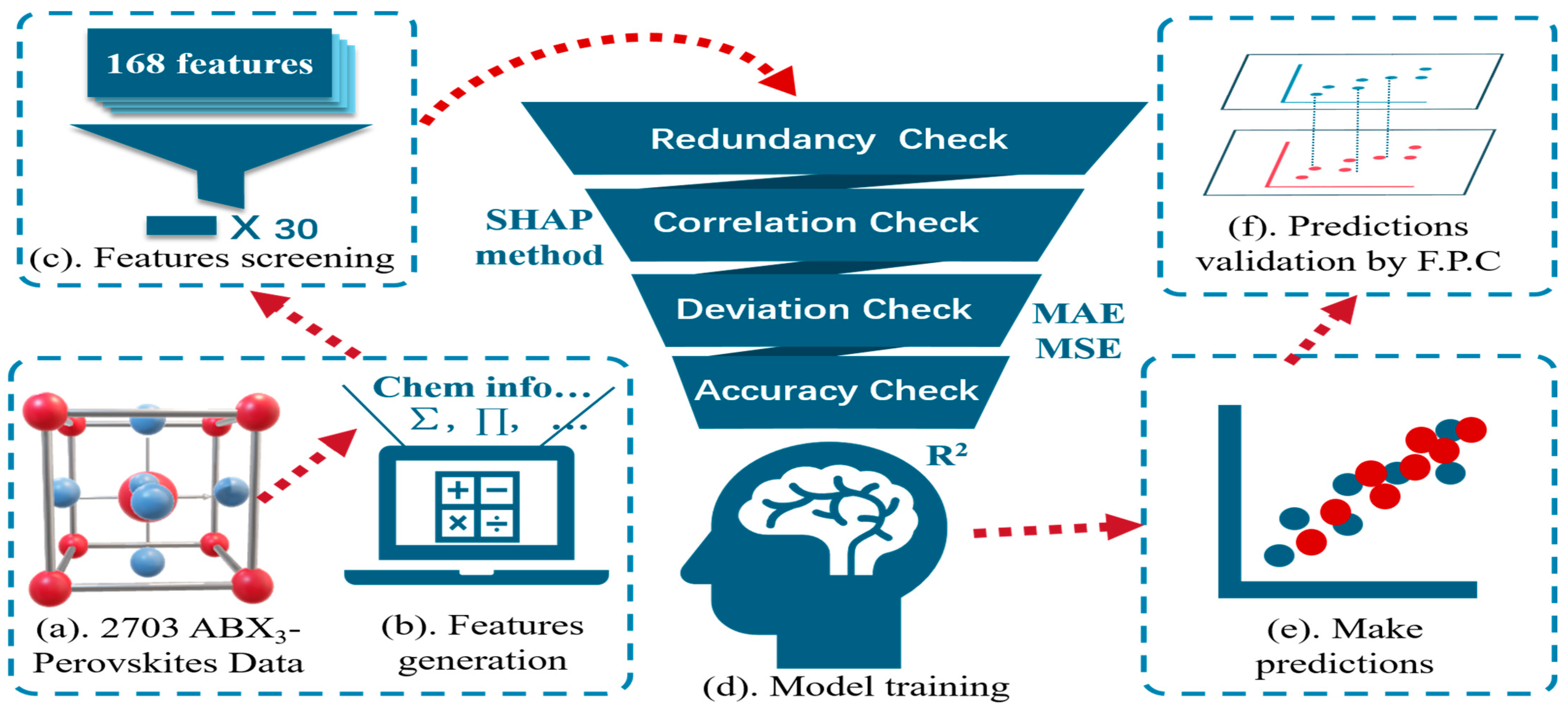
2. Methodology
2.1. Dataset Establishment
2.2. Feature Generation
2.3. Model Selection
2.4. Model Verification Means
3. Results and Discussion
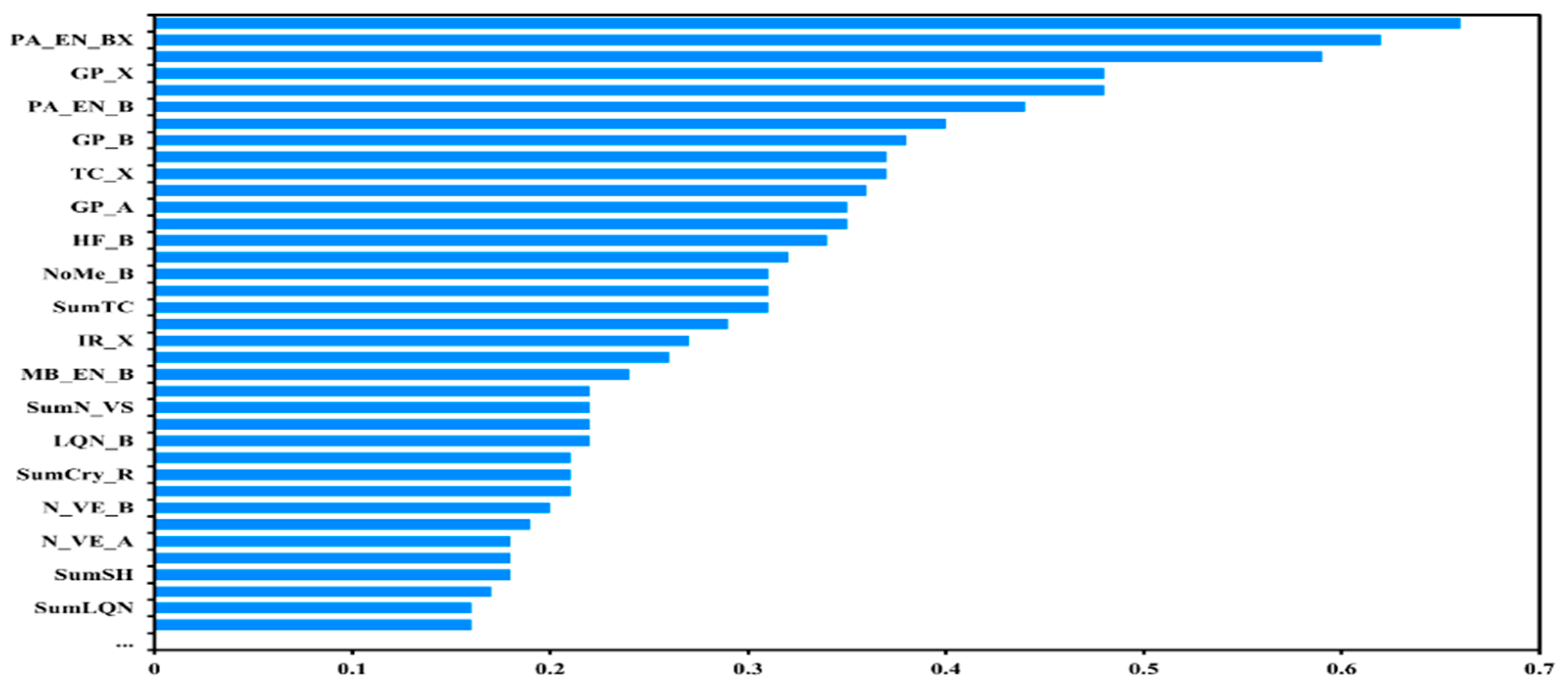
3.1. Data Processing and Feature Screening
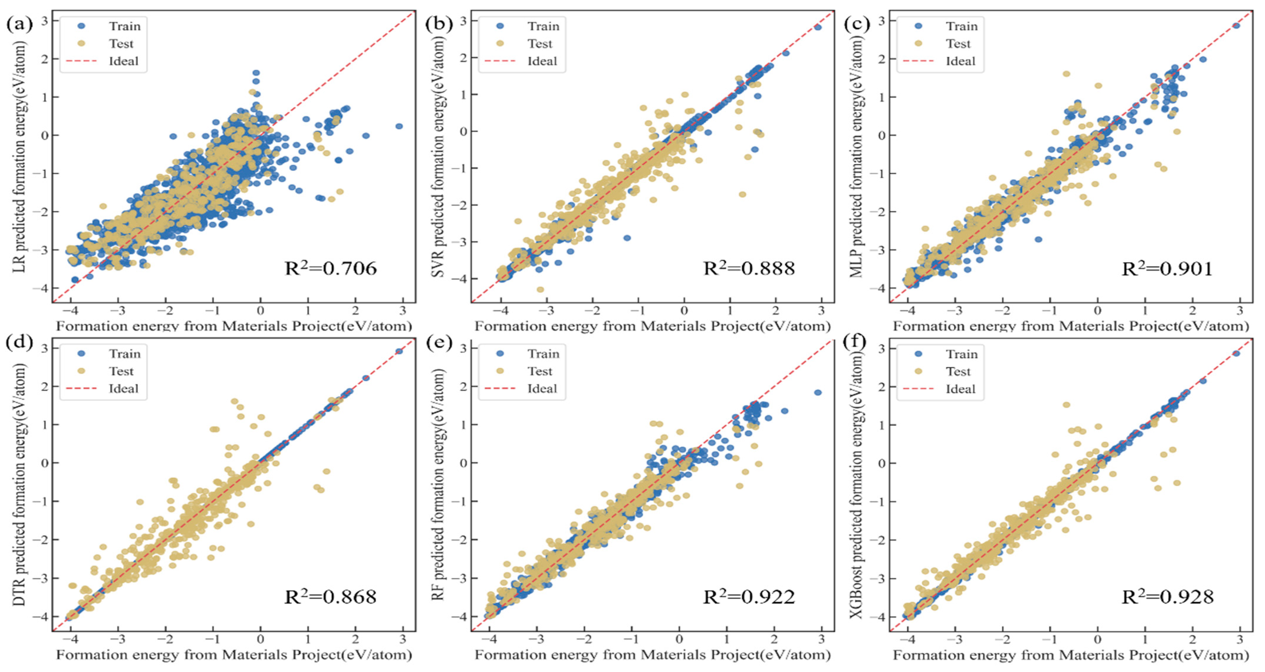
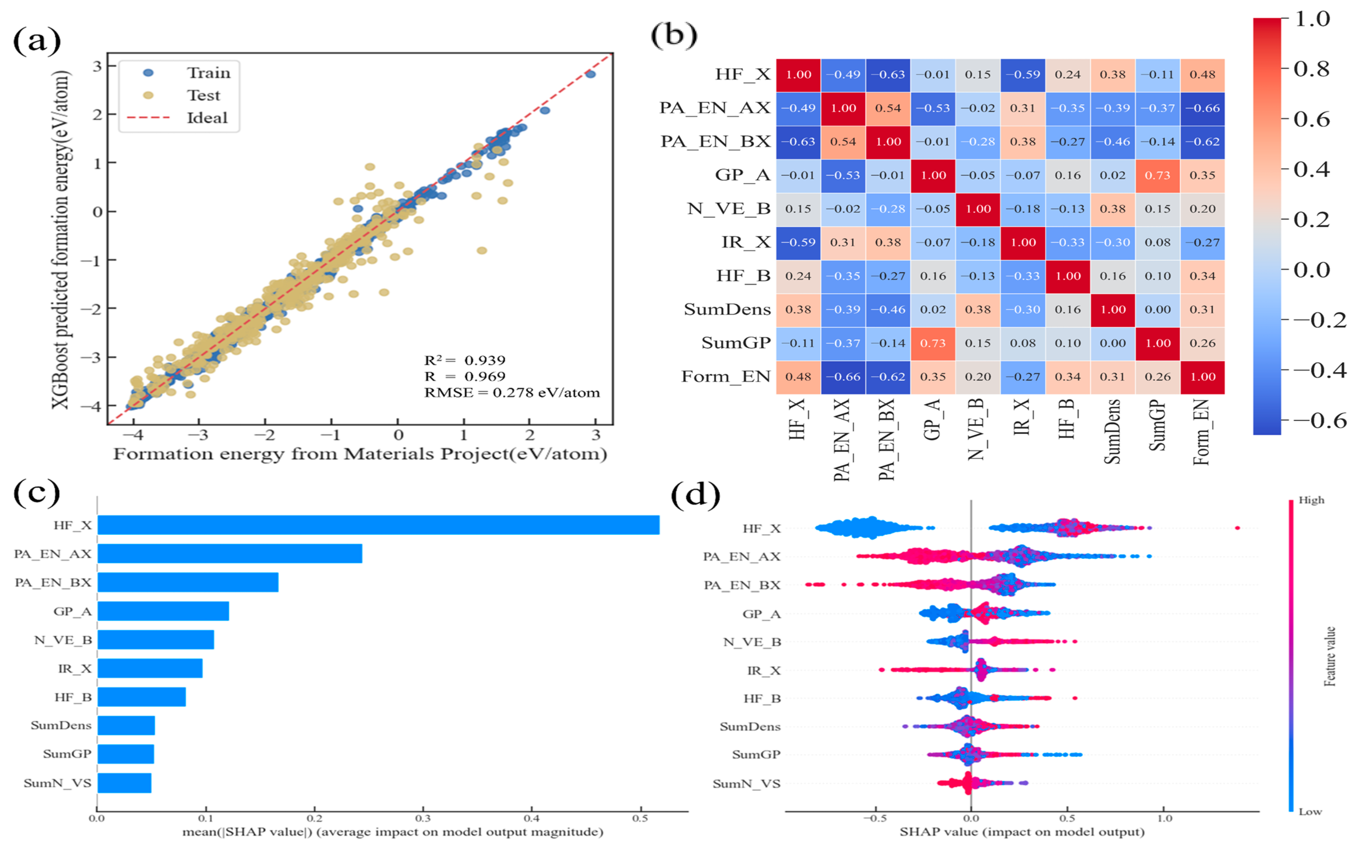
3.2. Model Training and Performance Evaluation
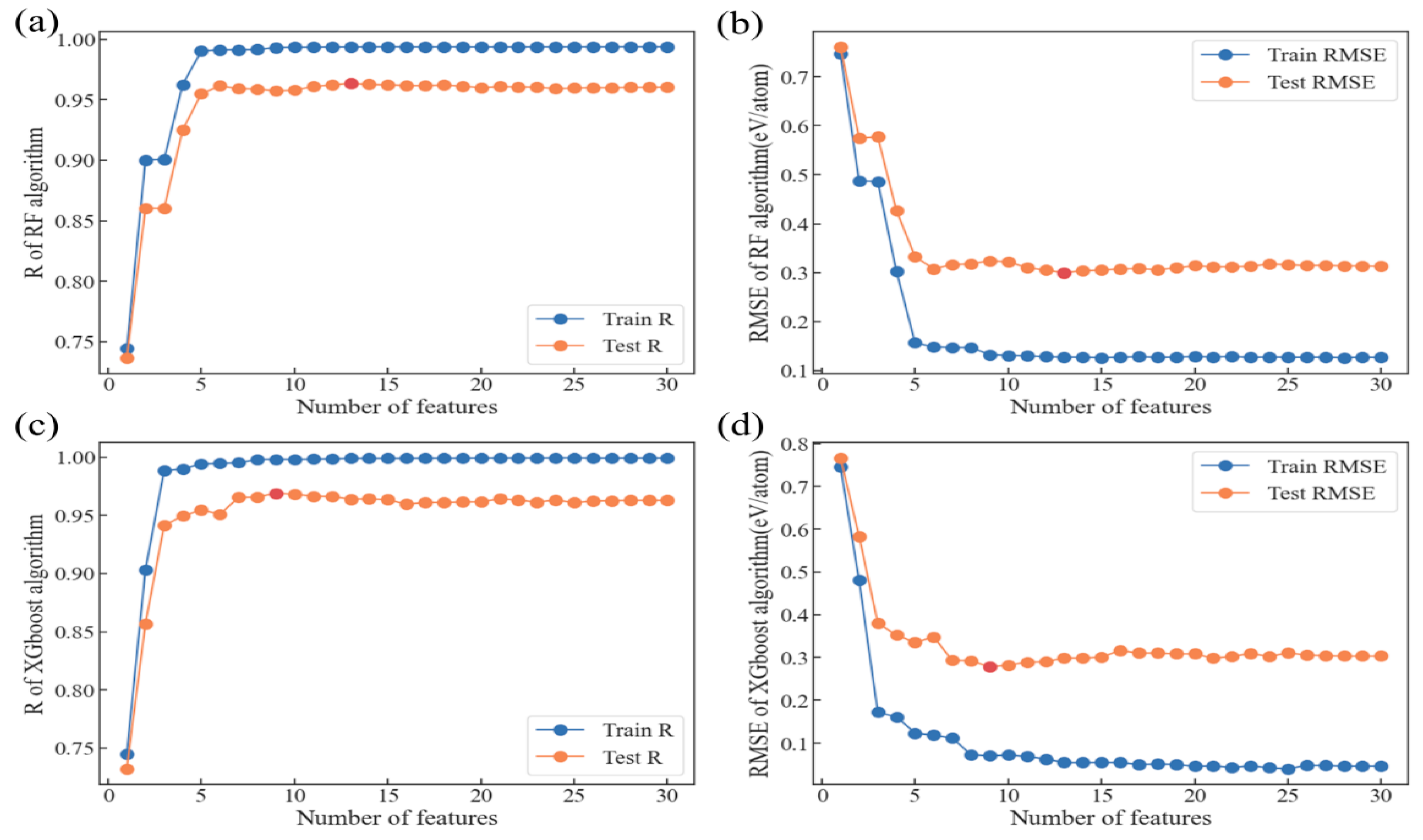
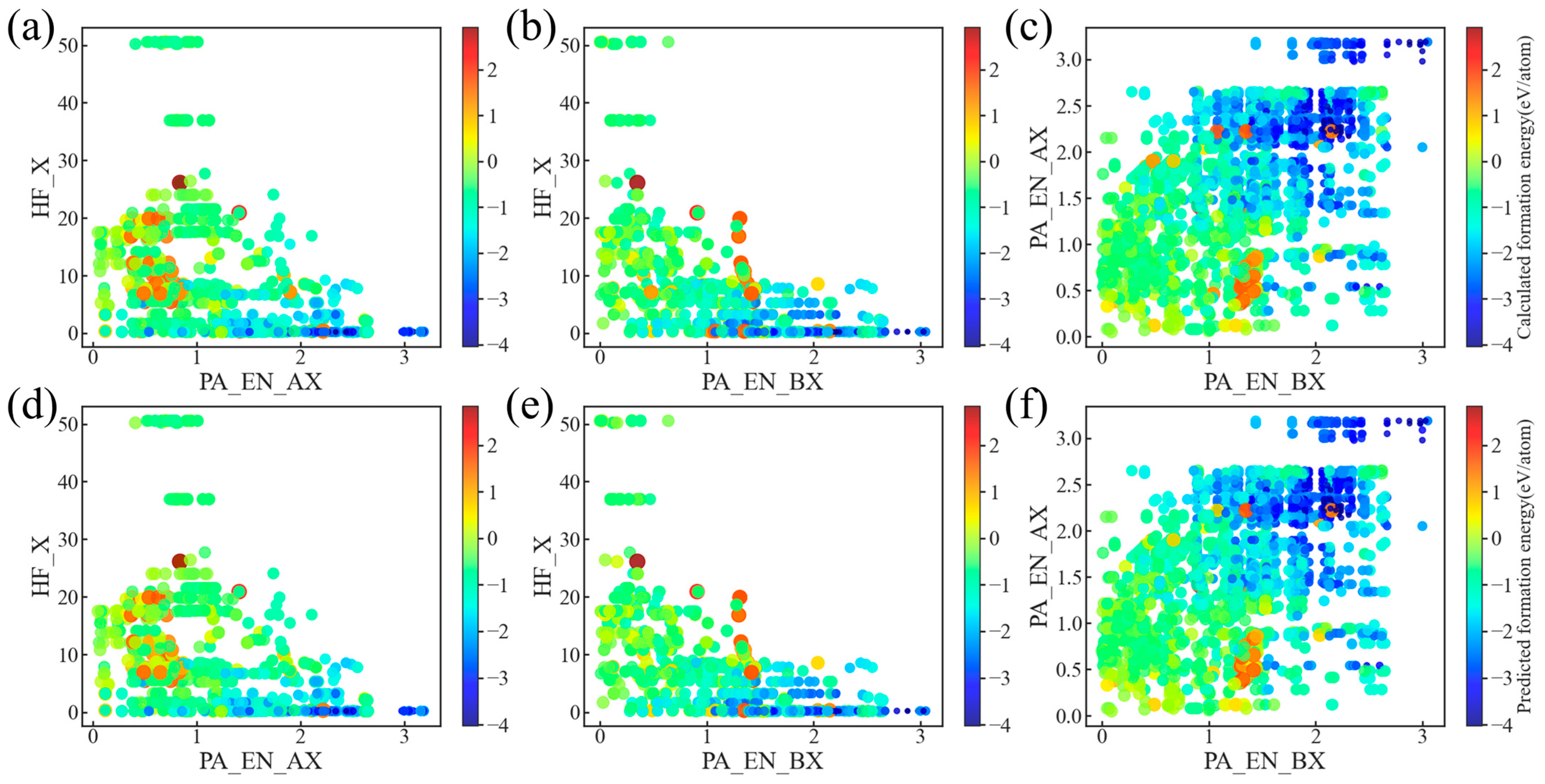
3.3. Model Optimization and Feature Analysis
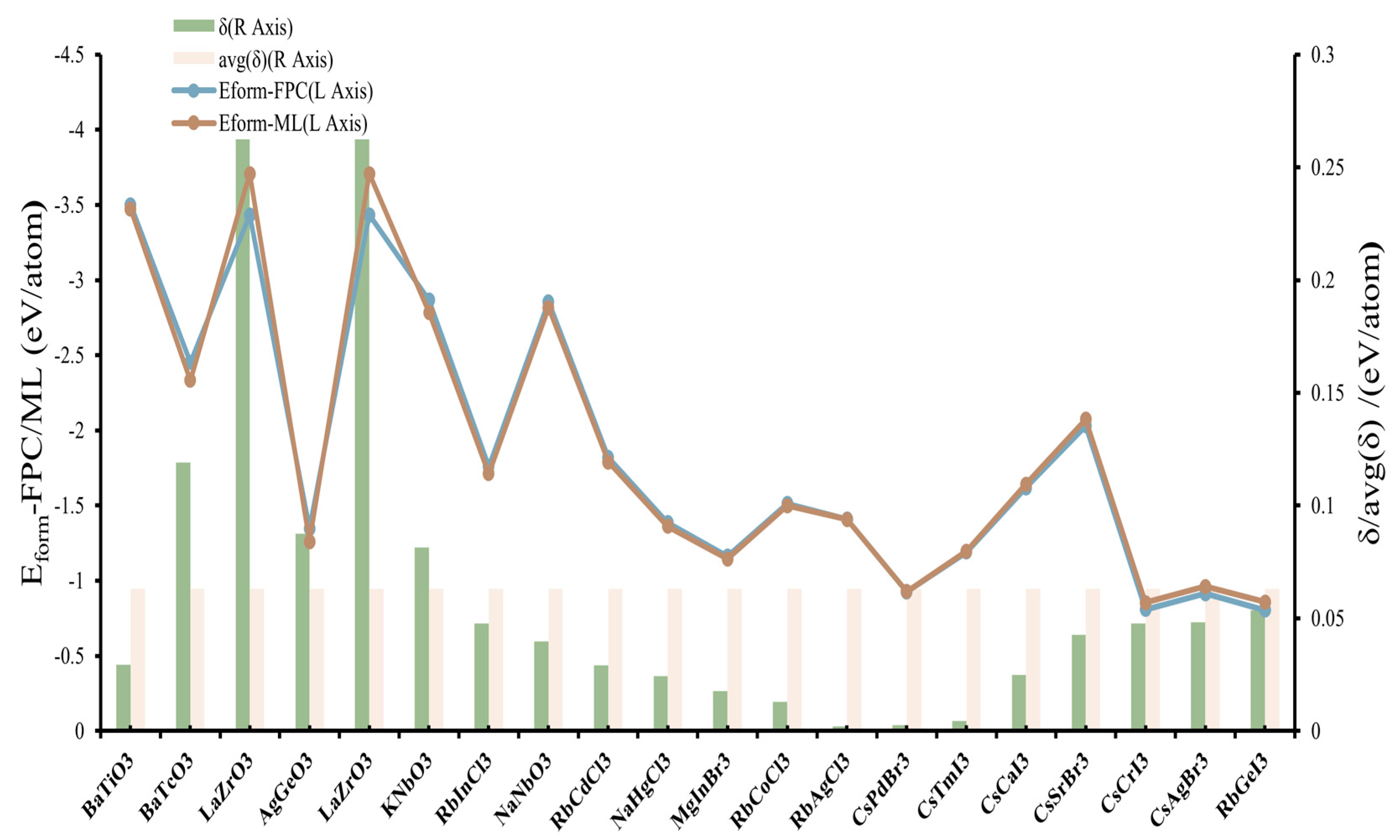
3.4. Model Validation
4. Conclusions
Supplementary Materials
Author Contributions
Funding
Institutional Review Board Statement
Informed Consent Statement
Data Availability Statement
Acknowledgments
Conflicts of Interest
References
- Tao, Q.; Xu, P.; Li, M.; Lu, W. Machine learning for perovskite materials design and discovery. Npj Comput. Mater. 2021, 7, 23. [Google Scholar] [CrossRef]
- Liu, Y.; Tan, X.; Liang, J.; Han, H.; Xiang, P.; Yan, W. Machine Learning for Perovskite Solar Cells and Component Materials: Key Technologies and Prospects. Adv. Funct. Mater. 2023, 33, 2214271. [Google Scholar] [CrossRef]
- Liu, D.; Shao, Z.; Li, C.; Pang, S.; Yan, Y.; Cui, G. Structural Properties and Stability of Inorganic CsPbI3 Perovskites. Small Struct. 2021, 2, 2000089. [Google Scholar] [CrossRef]
- Xiang, W.; Liu, S.F.; Tress, W. A review on the stability of inorganic metal halide perovskites: Challenges and opportunities for stable solar cells. Energy Environ. Sci. 2021, 14, 2090–2113. [Google Scholar] [CrossRef]
- Zhu, Y.; Zhang, J.; Qu, Z.; Jiang, S.; Liu, Y.; Wu, Z.; Yang, F.; Hu, W.; Xu, Z.; Dai, Y. Accelerating stability of ABX3 perovskites analysis with machine learning. Ceram. Int. 2024, 50, 6250–6258. [Google Scholar] [CrossRef]
- Ouedraogo, N.A.N.; Chen, Y.; Xiao, Y.Y.; Meng, Q.; Han, C.B.; Yan, H.; Zhang, Y. Stability of all-inorganic perovskite solar cells. Nano Energy 2020, 67, 104249. [Google Scholar] [CrossRef]
- Wang, Z.; Zhang, J.; Guo, W.; Xiang, W.; Hagfeldt, A. Formation and Stabilization of Inorganic Halide Perovskites for Photovoltaics. Matter 2021, 4, 528–551. [Google Scholar] [CrossRef]
- Yu, S.; Yao, K.; Tay, F.E.H. Observations and Analyses on the Thermal Stability of (1-x)Pb(Zn1/3Nb2/3)O3−xPbTiO3 Thin Films. Chem. Mater. 2007, 19, 4373–4377. [Google Scholar] [CrossRef]
- Yu, S.; Yao, K.; Tay, F.E.H. Structure and Properties of (1−x)PZN−xPT Thin Films with Perovskite Phase Promoted by Polyethylene Glycol. Chem. Mater. 2006, 18, 5343–5350. [Google Scholar] [CrossRef]
- Li, F.; Pei, Y.; Xiao, F.; Zeng, T.; Yang, Z.; Xu, J.; Sun, J.; Peng, B.; Liu, M. Tailored dimensionality to regulate the phase stability of inorganic cesium lead iodide perovskites. Nanoscale 2018, 10, 6318–6322. [Google Scholar] [CrossRef]
- Yao, K.; Yu, S.; Tay, F.E.H. Preparation of perovskite Pb(Zn1∕3Nb2∕3)O3-based thin films from polymer-modified solution precursors. Appl. Phys. Lett. 2006, 88, 052904. [Google Scholar] [CrossRef]
- Yan, S.; Cao, Z.; Liu, Q.; Gao, Y.; Zhang, H.; Li, G. Enhanced piezoelectric activity around orthorhombic-tetragonal phase boundary in multielement codoping BaTiO3. J. Alloys Compd. 2022, 923, 166398. [Google Scholar] [CrossRef]
- Coondoo, I.; Alikin, D.; Abramov, A.; Figueiras, F.G.; Shur, V.Y.; Miranda, G. Exploring the effect of low concentration of stannum in lead-free BCT-BZT piezoelectric compositions for energy related applications. J. Alloys Compd. 2023, 960, 170562. [Google Scholar] [CrossRef]
- Travis, W.; Glover, E.N.K.; Bronstein, H.; Scanlon, D.O.; Palgrave, R.G. On the application of the tolerance factor to inorganic and hybrid halide perovskites: A revised system. Chem. Sci. 2016, 7, 4548–4556. [Google Scholar] [CrossRef]
- Kieslich, G.; Sun, S.; Cheetham, A.K. Solid-state principles applied to organic–inorganic perovskites: New tricks for an old dog. Chem. Sci. 2014, 5, 4712–4715. [Google Scholar] [CrossRef]
- Kieslich, G.; Sun, S.; Cheetham, A.K. An extended Tolerance Factor approach for organic–inorganic perovskites. Chem. Sci. 2015, 6, 3430–3433. [Google Scholar] [CrossRef]
- Zhao, X.; Yang, J.; Fu, Y.; Yang, D.; Xu, Q.; Yu, L.; Wei, S.-H.; Zhang, L. Design of Lead-Free Inorganic Halide Perovskites for Solar Cells via Cation-Transmutation. J. Am. Chem. Soc. 2017, 139, 2630–2638. [Google Scholar] [CrossRef]
- Sun, Q.; Yin, W. Thermodynamic Stability Trend of Cubic Perovskites. J. Am. Chem. Soc. 2017, 139, 14905–14908. [Google Scholar] [CrossRef]
- King, D.J.M.; Middleburgh, S.C.; McGregor, A.G.; Cortie, M.B. Predicting the formation and stability of single phase high-entropy alloys. Acta Mater. 2016, 104, 172–179. [Google Scholar] [CrossRef]
- Ong, S.P.; Wang, L.; Kang, B.; Ceder, G. Li−Fe−P−O2 Phase Diagram from First Principles Calculations. Chem. Mater. 2008, 20, 1798–1807. [Google Scholar] [CrossRef]
- Miura, A.; Bartel, C.J.; Goto, Y.; Mizuguchi, Y.; Moriyoshi, C.; Kuroiwa, Y.; Wang, Y.; Yaguchi, T.; Shirai, M.; Nagao, M.; et al. Observing and Modeling the Sequential Pairwise Reactions that Drive Solid-State Ceramic Synthesis. Adv. Mater. 2021, 33, 2100312. [Google Scholar] [CrossRef]
- Liang, Y.; Chen, M.; Wang, Y.; Jia, H.; Lu, T.; Xie, F.; Cai, G.; Wang, Z.; Meng, S.; Liu, M. A universal model for accurately predicting the formation energy of inorganic compounds. Sci. China Mater. 2022, 66, 343–351. [Google Scholar] [CrossRef]
- Feng, Y.; Wu, J.; Chi, Q.; Li, W.; Yu, Y.; Fei, W. Defects and Aliovalent Doping Engineering in Electroceramics. Chem. Rev. 2020, 120, 1710–1787. [Google Scholar] [CrossRef]
- Monika; Pachori, S.; Agrawal, R.; Choudhary, B.L.; Verma, A.S. An efficient and stable lead-free organic–inorganic tin iodide perovskite for photovoltaic device: Progress and challenges. Energy Rep. 2022, 8, 5753–5763. [Google Scholar] [CrossRef]
- Saidaminov, M.I.; Kim, J.; Jain, A.; Quintero-Bermudez, R.; Tan, H.; Long, G.; Tan, F.; Johnston, A.; Zhao, Y.; Voznyy, O.; et al. Suppression of atomic vacancies via incorporation of isovalent small ions to increase the stability of halide perovskite solar cells in ambient air. Nat. Energy 2018, 3, 648–654. [Google Scholar] [CrossRef]
- Zhou, Y.; Zhao, Y. Chemical stability and instability of inorganic halide perovskites. Energy Environ. Sci. 2019, 12, 1495–1511. [Google Scholar] [CrossRef]
- Hu, M.; Chen, M.; Guo, P.; Zhou, H.; Deng, J.; Yao, Y.; Jiang, Y.; Gong, J.; Dai, Z.; Qian, F.; et al. Sub-1.4eV bandgap inorganic perovskite solar cells with long-term stability. Nat. Commun. 2020, 11, 151. [Google Scholar] [CrossRef]
- Sutton, R.J.; Filip, M.R.; Haghighirad, A.A.; Sakai, N.; Wenger, B.; Giustino, F.; Snaith, H.J. Cubic or Orthorhombic? Revealing the Crystal Structure of Metastable Black-Phase CsPbI3 by Theory and Experiment. ACS Energy Lett. 2018, 3, 1787–1794. [Google Scholar] [CrossRef]
- Nagabhushana, G.P.; Shivaramaiah, R.; Navrotsky, A. Direct calorimetric verification of thermodynamic instability of lead halide hybrid perovskites. Proc. Natl. Acad. Sci. USA 2016, 113, 7717–7721. [Google Scholar] [CrossRef]
- Alhashmi, A.; Kanoun, M.B.; Goumri-Said, S. Machine Learning for Halide Perovskite Materials ABX3 (B = Pb, X = I, Br, Cl) Assessment of Structural Properties and Band Gap Engineering for Solar Energy. Materials 2023, 16, 2657. [Google Scholar] [CrossRef]
- Raccuglia, P.; Elbert, K.C.; Adler, P.; Falk, C.; Wenny, M.B.; Mollo, A.; Zeller, M.; Friedler, S.A.; Schrier, J.; Norquist, A.J. Machine-learning-assisted materials discovery using failed experiments. Nature 2016, 533, 73–76. [Google Scholar] [CrossRef]
- Agrawal, A.; Choudhary, A. Perspective: Materials informatics and big data: Realization of the “fourth paradigm” of science in materials science. APL Mater. 2016, 4, 053208. [Google Scholar] [CrossRef]
- Singh, M.; Tiwari, J.P. Tailoring of the Band Gap of MA3 Bi2 I9 through Doping at A as well as X Sites (of ABX3 Structure): Futuristic Material for Multijunction Solar Cells. ACS Appl. Energy Mater. 2025, 8, 6264–6269. [Google Scholar] [CrossRef]
- Shimul, A.I.; Sarker, S.R.; Ghosh, A.; Zaman, M.T.U.; Alrafai, H.A.; Hassan, A.A. Examining the optoelectronic and photovoltaic characteristics of Mg3SbM3 (M = F, Cl, Br) perovskites with diverse charge transport layers through numerical optimization and machine learning techniques. Inorg. Chem. Commun. 2025, 179, 114737. [Google Scholar] [CrossRef]
- Zhai, X.; Chen, M. Accelerated Design for Perovskite-Oxide-Based Photocatalysts Using Machine Learning Techniques. Materials 2024, 17, 3026. [Google Scholar] [CrossRef]
- Shafiq, M.; Amin, B.; Jehangir, M.A.; Chaudhry, A.R.; Murataza, G. First-principle calculations to investigate mechanical and acoustical properties of predicted stable halide Perovskite ABX3. J. Mol. Graph. Model. 2024, 133, 108861. [Google Scholar] [CrossRef]
- Pyun, D.; Lee, S.; Lee, S.; Jeong, S.-H.; Hwang, J.-K.; Kim, K.; Kim, Y.; Nam, J.; Cho, S.; Hwang, J.-S.; et al. Machine Learning-Assisted Prediction of Ambient-Processed Perovskite Solar Cells’ Performances. Energies 2024, 17, 5998. [Google Scholar] [CrossRef]
- Hongyu, C.; Liang, C.; Wensheng, Y. Stability Challenges in Industrialization of Perovskite Photovoltaics: From Atomic-Scale View to Module Encapsulation. Adv. Funct. Mater. 2024, 35, 2412389. [Google Scholar] [CrossRef]
- Ahamed, A.I.; Siam, J.; Rabah, B.; Riyad, K.; Rifat, R.; Moamen, S.R.; Hasan, M.S.S.; Amnah, M.A.; Azizur, M.R.; Alamgir, M.H.; et al. Exploring ACdX3 Perovskites: DFT Analysis of Stability, Electronic, Optical, and Mechanical Properties for Solar Applications. J. Inorg. Organomet. Polym. Mater. 2025, 1–26. [Google Scholar] [CrossRef]
- Himanen, L.; Geurts, A.; Foster, A.S.; Rinke, P. Data-Driven Materials Science: Status, Challenges, and Perspectives. Adv. Sci. 2019, 6, 1900808. [Google Scholar] [CrossRef]
- Vivanco-Benavides, L.E.; Martínez-González, C.L.; Mercado-Zúñiga, C.; Torres-Torres, C. Machine learning and materials informatics approaches in the analysis of physical properties of carbon nanotubes: A review. Comput. Mater. Sci. 2022, 201, 110939. [Google Scholar] [CrossRef]
- Bauer, S.; Benner, P.; Bereau, T.; Blum, V.; Boley, M.; Carbogno, C.; Catlow, C.R.A.; Dehm, G.; Eibl, S.; Ernstorfer, R.; et al. Roadmap on Data-Centric Materials Science. arXiv 2024, arXiv:2402.10932. [Google Scholar] [CrossRef]
- Chong, S.S.; Ng, Y.S.; Wang, H.-Q.; Zheng, J.-C. Advances of machine learning in materials science: Ideas and techniques. Front. Phys. 2023, 19, 13501. [Google Scholar] [CrossRef]
- Obasi, C.; Oranu, O. Exploring Machine Learning Algorithms and Their Applications in Materials Science. J. Comput. Intell. Mater. Sci. 2024, 2, 23–35. [Google Scholar] [CrossRef]
- Liu, Y.; Zhao, T.; Ju, W.; Shi, S. Materials discovery and design using machine learning. J. Mater. 2017, 3, 159–177. [Google Scholar] [CrossRef]
- Batra, R. Accurate machine learning in materials science facilitated by using diverse data sources. Nature 2021, 589, 524–525. [Google Scholar] [CrossRef]
- Liu, Y.; Niu, C.; Wang, Z.; Gan, Y.; Zhu, Y.; Sun, S.; Shen, T. Machine learning in materials genome initiative: A review. J. Mater. Sci. Technol. 2020, 57, 113–122. [Google Scholar] [CrossRef]
- Suh, C.; Fare, C.; Warren, J.A.; Pyzer-Knapp, E.O. Evolving the Materials Genome: How Machine Learning Is Fueling the Next Generation of Materials Discovery. Annu. Rev. Mater. Res. 2020, 50, 1–25. [Google Scholar] [CrossRef]
- Ramprasad, R.; Batra, R.; Pilania, G.; Mannodi-Kanakkithodi, A.; Kim, C. Machine learning in materials informatics: Recent applications and prospects. npj Comput. Mater. 2017, 3, 54. [Google Scholar] [CrossRef]
- Jianxin, X. Prospects of materials genome engineering frontiers. Mater. Genome Eng. Adv. 2023, 1, e17. [Google Scholar] [CrossRef]
- Jiang, X.; Fu, H.; Bai, Y.; Jiang, L.; Zhang, H.; Wang, W.; Yun, P.; He, J.; Xue, D.; Lookman, T.; et al. Interpretable Machine Learning Applications: A Promising Prospect of AI for Materials. Adv. Funct. Mater. 2025, 2507734. [Google Scholar] [CrossRef]
- Xie, J.; Su, Y.; Zhang, D.; Feng, Q. A Vision of Materials Genome Engineering in China. Engineering 2022, 10, 10–12. [Google Scholar] [CrossRef]
- Xu, P.; Ji, X.; Li, M.; Lu, W. Small data machine learning in materials science. npj Comput. Mater. 2023, 9, 42. [Google Scholar] [CrossRef]
- Pouchard, L.U.; Lin, Y.U.; Van Dam, H.U. Replicating Machine Learning Experiments in Materials Science. Adv. Parallel Comput. 2020, 36, 743–755. [Google Scholar] [CrossRef]
- Andrew, S.; Vinayak, B.; Qianxiang, A.; Chad, R. Challenges in Information-Mining the Materials Literature: A Case Study and Perspective. Chem. Mater. 2022, 34, 4821–4827. [Google Scholar] [CrossRef]
- Belsky, A.; Hellenbrandt, M.; Karen, V.L.; Luksch, P. New developments in the Inorganic Crystal Structure Database (ICSD): Accessibility in support of materials research and design. Acta Crystallogr. Sect. B Struct. Sci. 2002, 58, 364–369. [Google Scholar] [CrossRef]
- Jain, A.; Ong, S.; Hautier, G.; Chen, W.; Richards, W.; Dacek, S.; Cholia, S.; Gunter, D.; Skinner, D.; Ceder, G.; et al. Commentary: The Materials Project: A materials genome approach to accelerating materials innovation. APL Mater. 2013, 1, 011002. [Google Scholar] [CrossRef]
- Kirklin, S. The Open Quantum Materials Database (OQMD): Assessing the accuracy of DFT formation energies. npj Comput. Mater. 2015, 15, 15010. [Google Scholar] [CrossRef]
- Pizzi, G.; Cepellotti, A.; Sabatini, R.; Marzari, N.; Kozinsky, B. AiiDA: Automated interactive infrastructure and database for computational science. Comput. Mater. Sci. 2016, 111, 218–230. [Google Scholar] [CrossRef]
- Pedregosa, F.; Varoquaux, G.; Gramfort, A.; Michel, V.; Thirion, B.; Grisel, O.; Blondel, M.; Prettenhofer, P.; Weiss, R.; Dubourg, V.; et al. Scikit-learn: Machine Learning in Python. J. Mach. Learn. Res. 2011, 12, 2825–2830. [Google Scholar]
- Chen, T.; Guestrin, C. XGBoost: A Scalable Tree Boosting System. In Proceedings of the 22nd ACM SIGKDD International Conference on Knowledge Discovery and Data Mining (KDD ’16), San Francisco, CA, USA, 13–17 August 2016; Association for Computing Machinery: New York, NY, USA, 2016; pp. 785–794. [Google Scholar] [CrossRef]
- Ketkar, N.; Moolayil, J. Deep Learning with Python: Learn Best Practices of Deep Learning Models with PyTorch; Apress: Berkeley, CA, USA, 2021. [Google Scholar] [CrossRef]
- Ward, L.; Agrawal, A.; Choudhary, A.; Wolverton, C. A general-purpose machine learning framework for predicting properties of inorganic materials. npj Comput. Mater. 2016, 2, 16028. [Google Scholar] [CrossRef]
- Ong, S.P.; Richards, W.D.; Jain, A.; Hautier, G.; Kocher, M.; Cholia, S.; Gunter, D.; Chevrier, V.L.; Persson, K.A.; Ceder, G. Python Materials Genomics (pymatgen): A robust, open-source python library for materials analysis. Comput. Mater. Sci. 2013, 68, 314–319. [Google Scholar] [CrossRef]
- He, J.; Yu, C.; Hou, Y.; Su, X.; Li, J.; Liu, C.; Xue, D.; Cao, J.; Su, Y.; Qiao, L.; et al. Accelerated discovery of high-performance piezocatalyst in BaTiO3-based ceramics via machine learning. Nano Energy 2022, 97, 107218. [Google Scholar] [CrossRef]
- Orio, M.; Pantazis, D.A.; Neese, F. Density functional theory. Photosynth. Res. 2009, 102, 443–453. [Google Scholar] [CrossRef]
- Bartel, C.J.; Weimer, A.W.; Lany, S.; Musgrave, C.B.; Holder, A.M. The role of decomposition reactions in assessing first-principles predictions of solid stability. npj Comput. Mater. 2019, 5, 4. [Google Scholar] [CrossRef]

| Model | MAE (eV/atom) | RMSE (eV/atom) | MSE | R2 | Pearson’s R Value | RMSE/Average () |
|---|---|---|---|---|---|---|
| LR | 0.473 | 0.607 | 0.369 | 0.706 | 0.843 | 0.353 |
| SVR | 0.229 | 0.375 | 0.140 | 0.888 | 0.942 | 0.221 |
| MLP | 0.221 | 0.352 | 0.124 | 0.901 | 0.950 | 0.214 |
| DTR | 0.229 | 0.407 | 0.165 | 0.868 | 0.934 | 0.235 |
| RF | 0.194 | 0.313 | 0.098 | 0.922 | 0.961 | 0.188 |
| XGBoost | 0.186 | 0.301 | 0.090 | 0.928 | 0.963 | 0.175 |
Disclaimer/Publisher’s Note: The statements, opinions and data contained in all publications are solely those of the individual author(s) and contributor(s) and not of MDPI and/or the editor(s). MDPI and/or the editor(s) disclaim responsibility for any injury to people or property resulting from any ideas, methods, instructions or products referred to in the content. |
© 2025 by the authors. Licensee MDPI, Basel, Switzerland. This article is an open access article distributed under the terms and conditions of the Creative Commons Attribution (CC BY) license (https://creativecommons.org/licenses/by/4.0/).
Share and Cite
Deng, Z.; Fang, K.; Guo, C.; Gong, Z.; Yue, H.; Zhang, H.; Li, K.; Guo, K.; Liu, Z.; Xie, B.; et al. Prediction of ABX3 Perovskite Formation Energy Using Machine Learning. Materials 2025, 18, 2927. https://doi.org/10.3390/ma18132927
Deng Z, Fang K, Guo C, Gong Z, Yue H, Zhang H, Li K, Guo K, Liu Z, Xie B, et al. Prediction of ABX3 Perovskite Formation Energy Using Machine Learning. Materials. 2025; 18(13):2927. https://doi.org/10.3390/ma18132927
Chicago/Turabian StyleDeng, Ziliang, Kailing Fang, Chong Guo, Zhichao Gong, Haojie Yue, Huacheng Zhang, Kang Li, Kun Guo, Zhiyong Liu, Bing Xie, and et al. 2025. "Prediction of ABX3 Perovskite Formation Energy Using Machine Learning" Materials 18, no. 13: 2927. https://doi.org/10.3390/ma18132927
APA StyleDeng, Z., Fang, K., Guo, C., Gong, Z., Yue, H., Zhang, H., Li, K., Guo, K., Liu, Z., Xie, B., Lu, J., Yao, K., & Tay, F. E. H. (2025). Prediction of ABX3 Perovskite Formation Energy Using Machine Learning. Materials, 18(13), 2927. https://doi.org/10.3390/ma18132927