


Modeling the Structure–Property Linkages Between the Microstructure and Thermodynamic Properties of Ceramic Particle-Reinforced Metal Matrix Composites Using a Materials Informatics Approach


Abstract
1. Introduction
2. Microstructure Model and Dataset
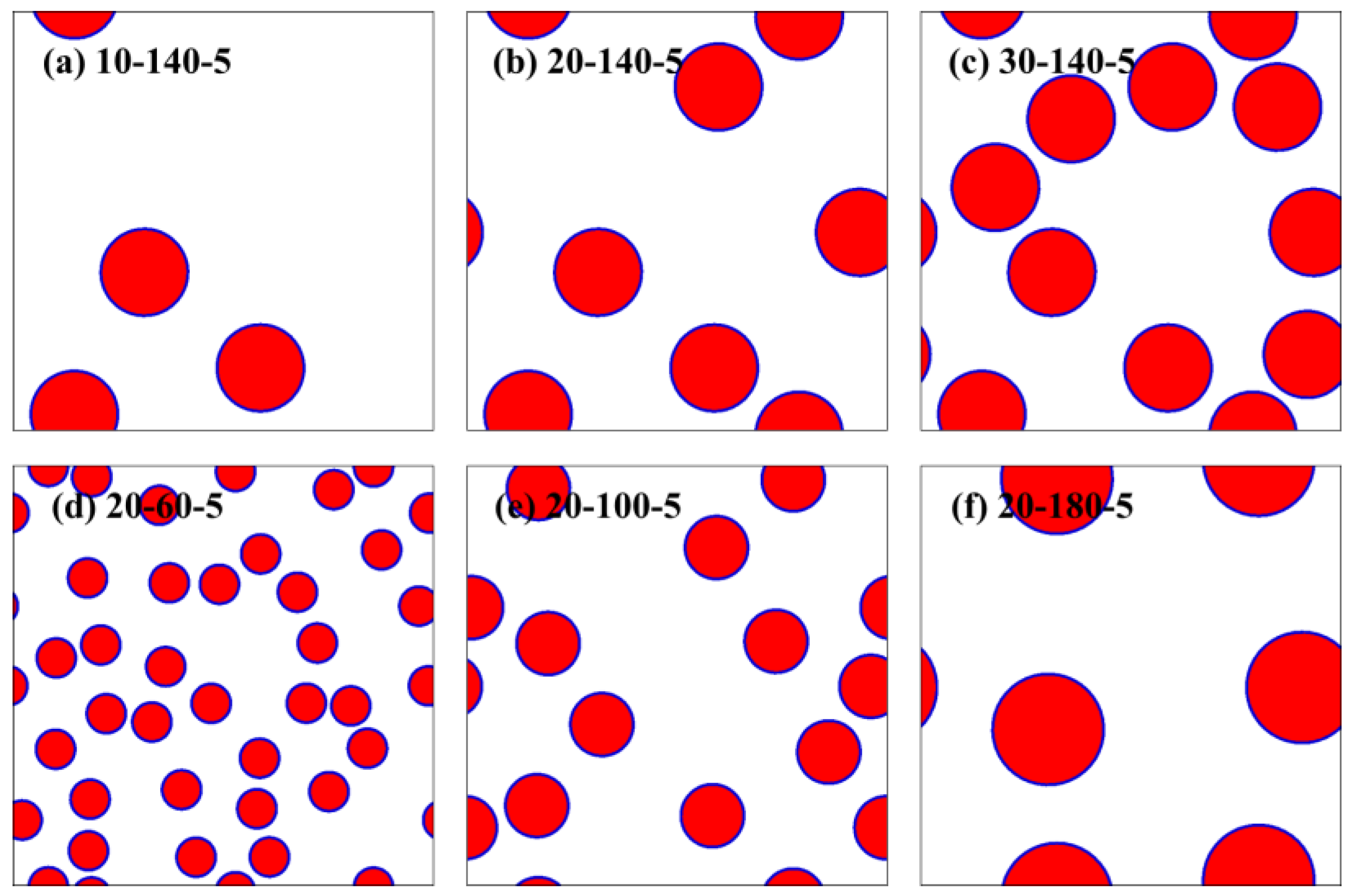
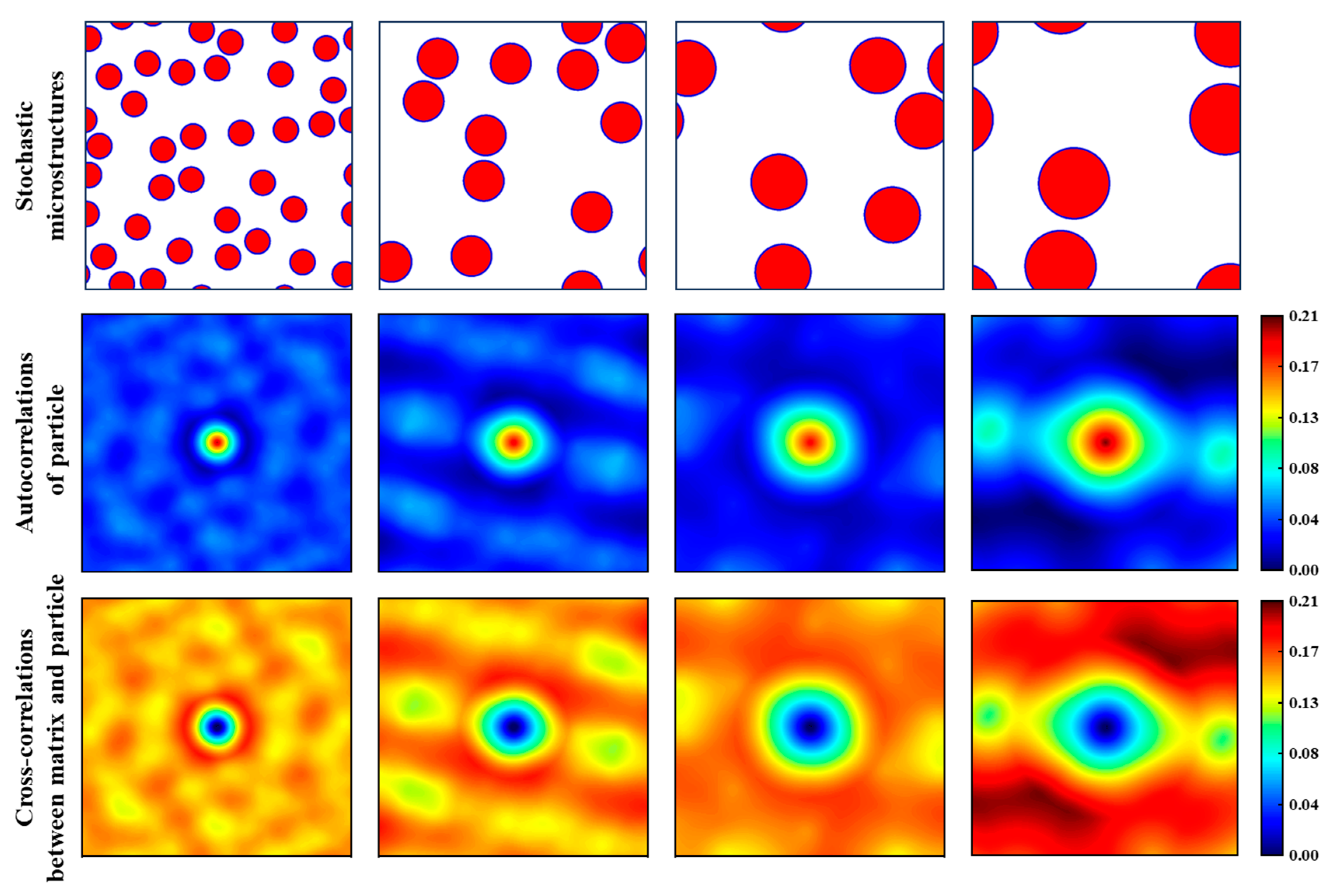
2.1. Generation of Stochastic Microstructures
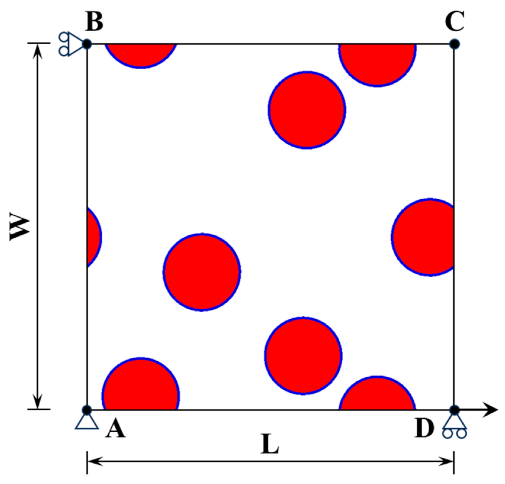
2.2. Model Solution Method
- (1)
- Periodic boundary conditions (PBCs)
- (2)
- Thermal conductivity
- (3)
- Coefficient of thermal expansion
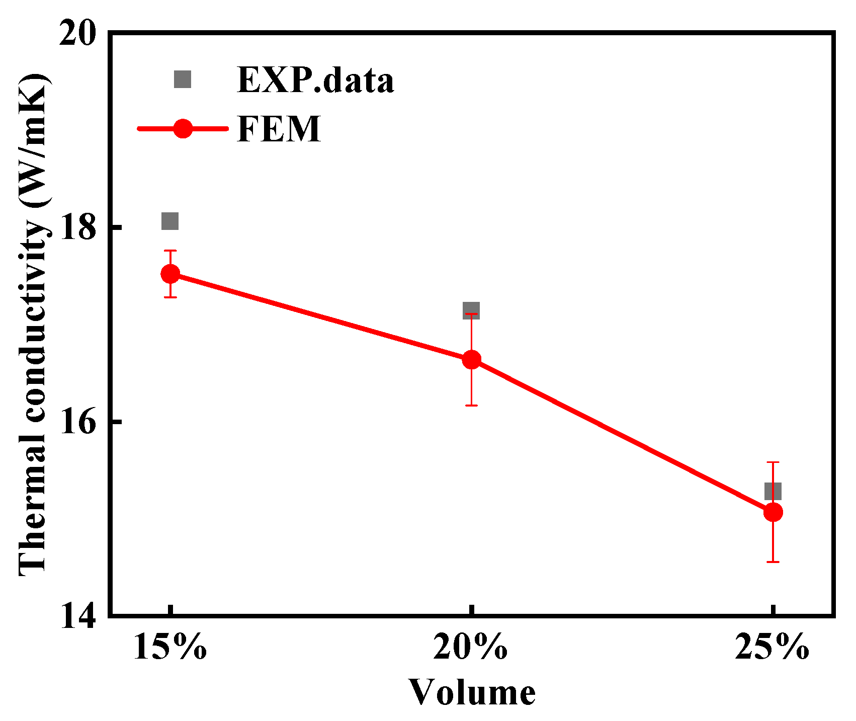
2.3. Evaluation of Thermodynamic Properties
3. Microstructure Dimensionality Reduction and Machine Learning Methods
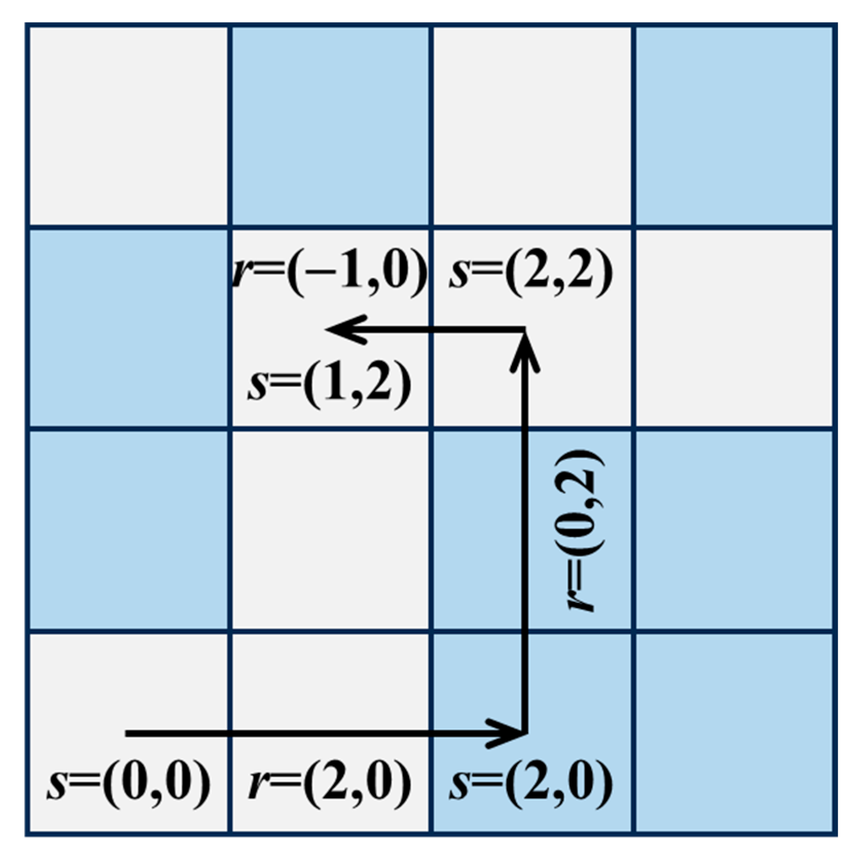
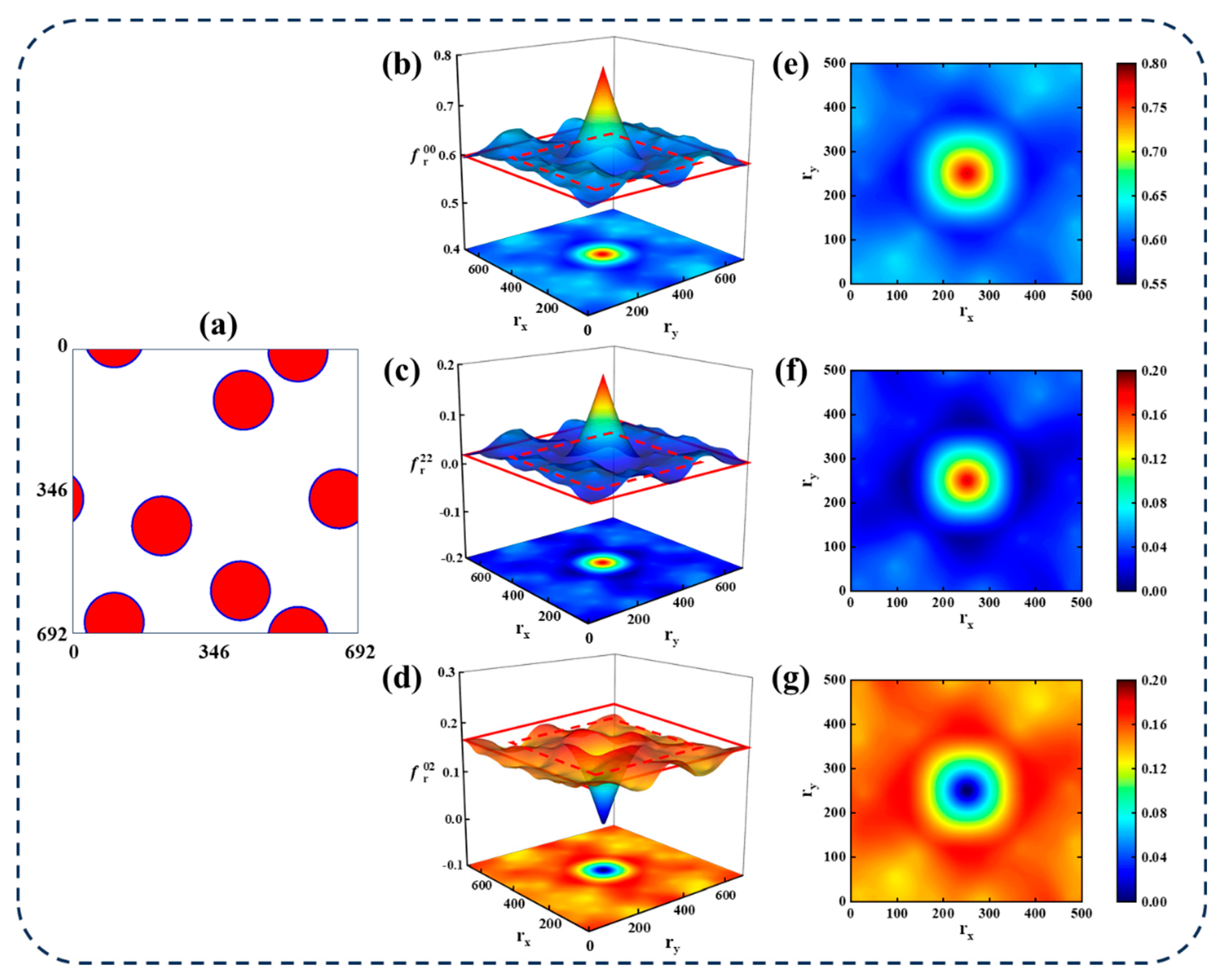
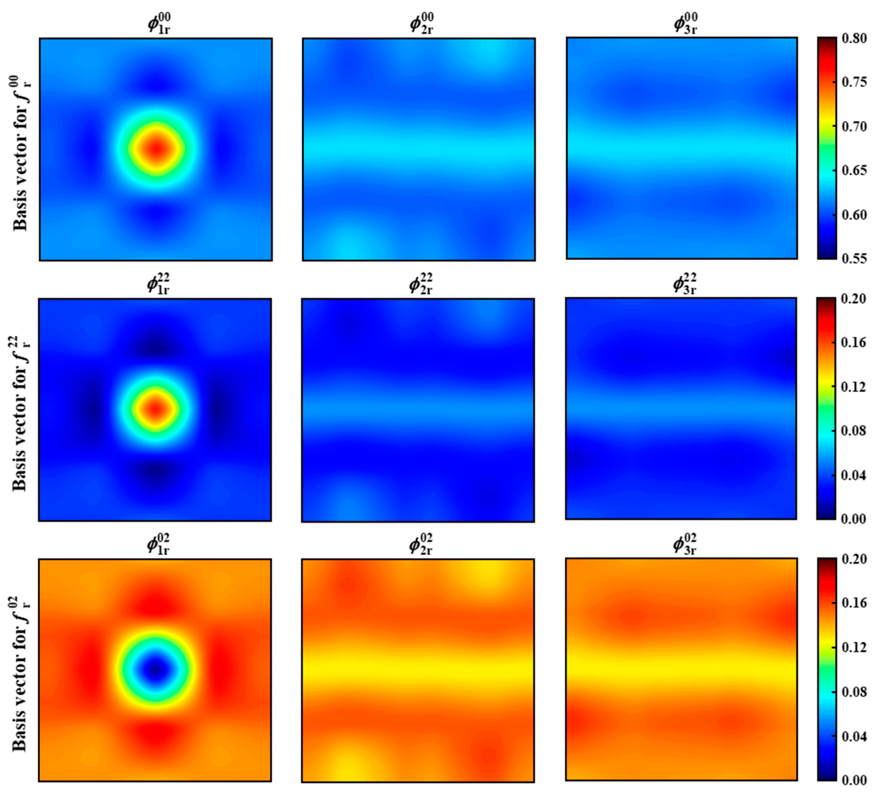
3.1. Statistical Representation of Microstructure
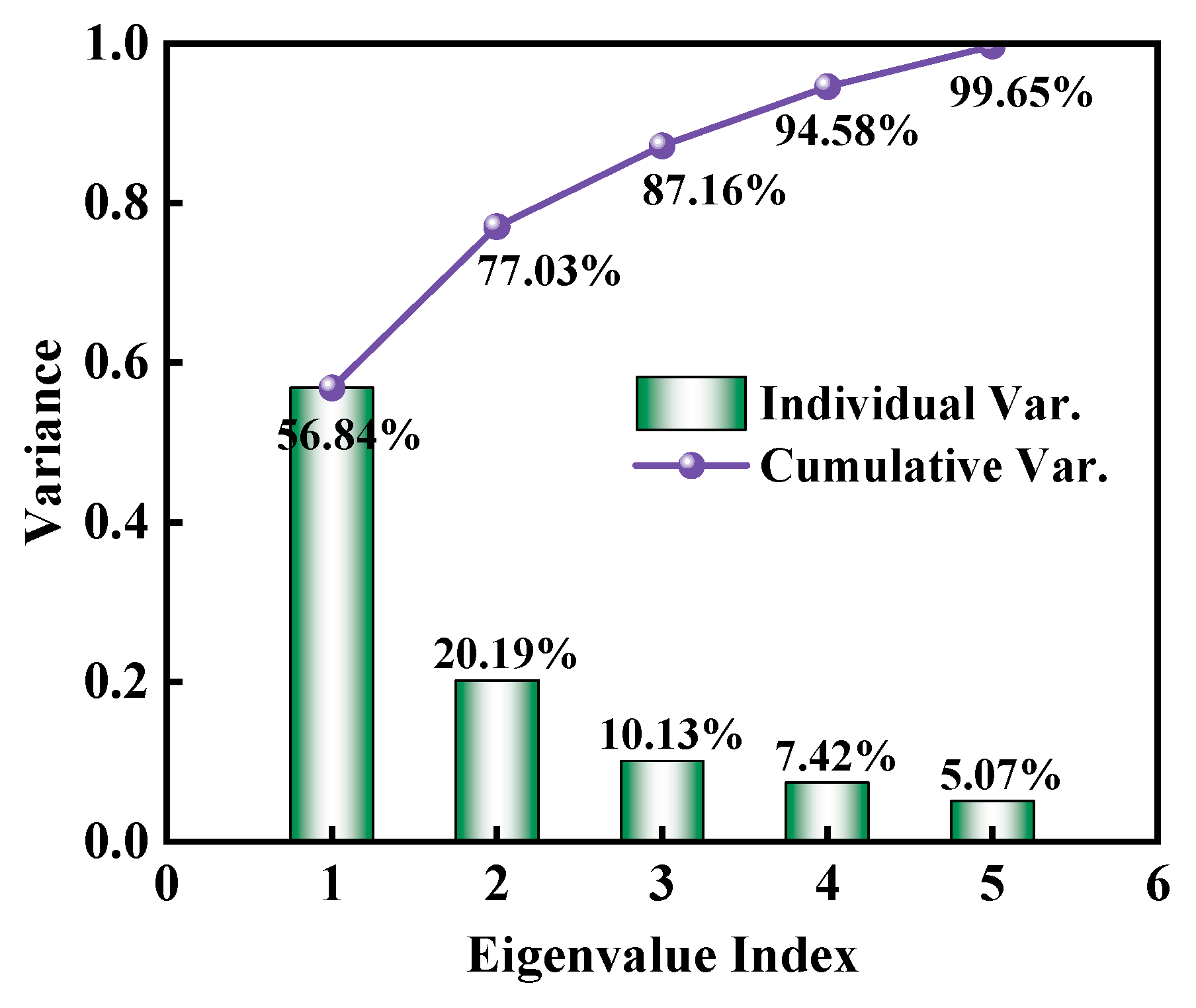
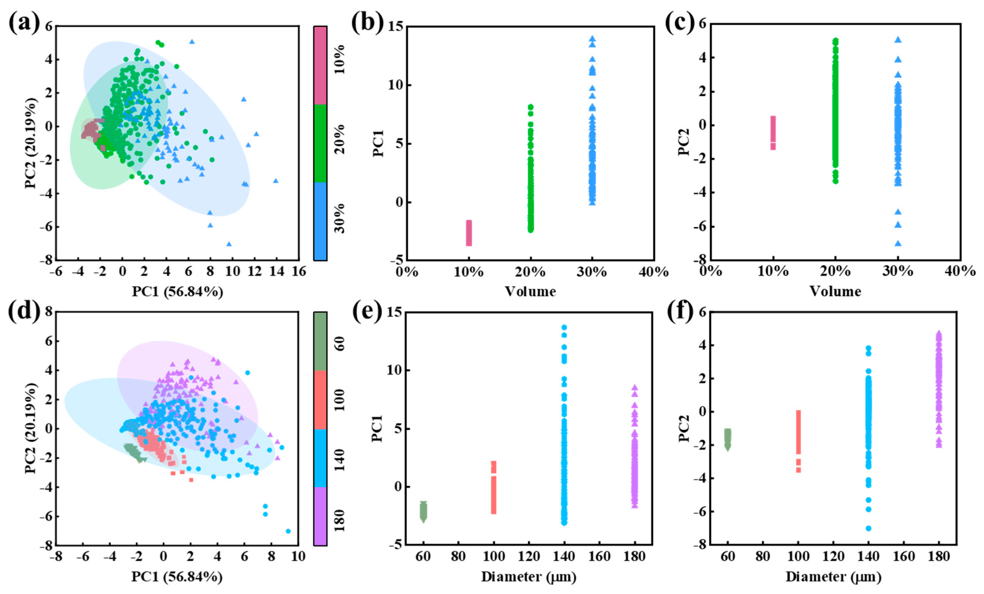
3.2. Dimensionality Reduction of Statistics
3.3. Machine Learning Methods
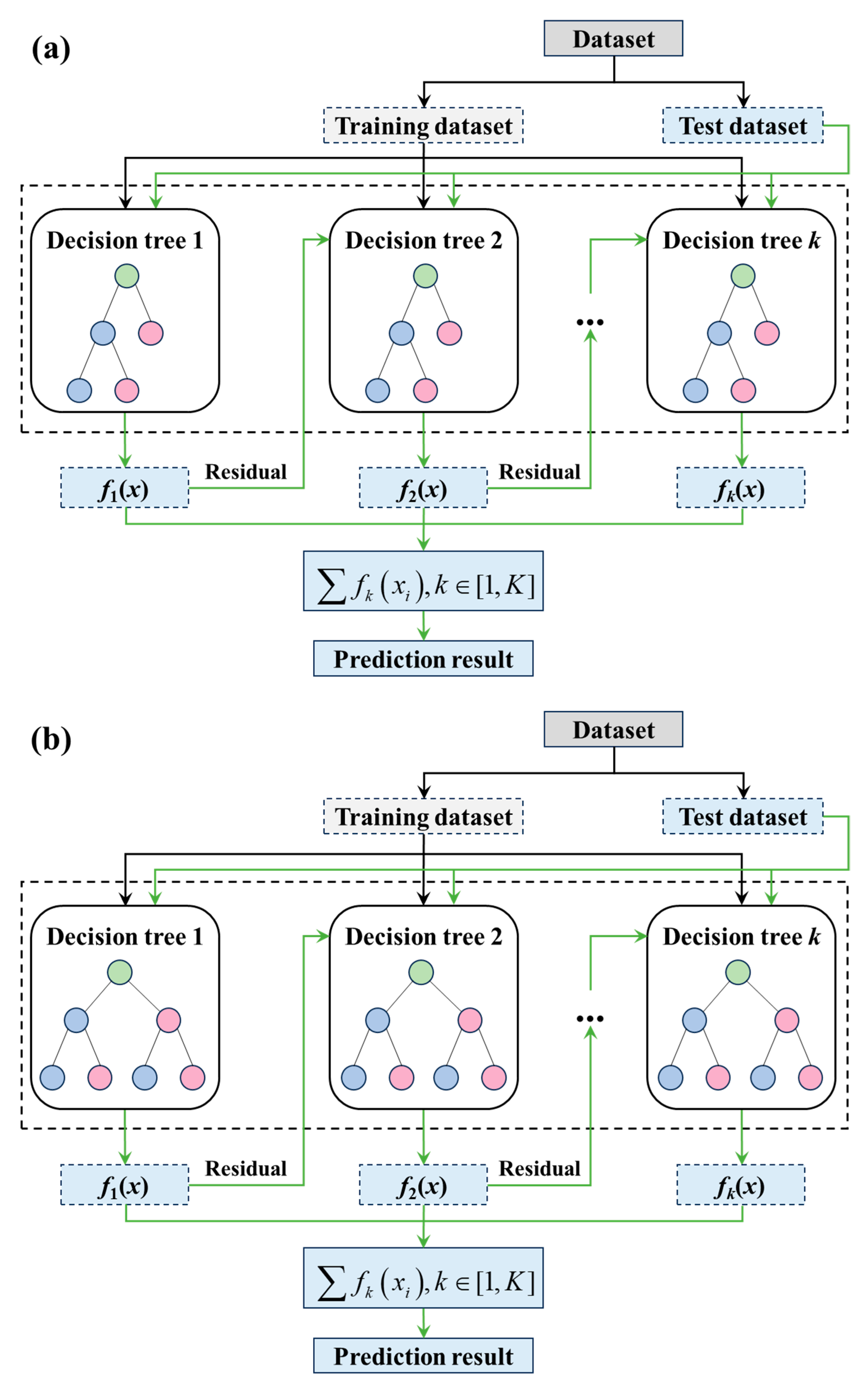
3.3.1. Machine Learning Models
- (1)
- XGBoost
- (2)
- CatBoost
- (3)
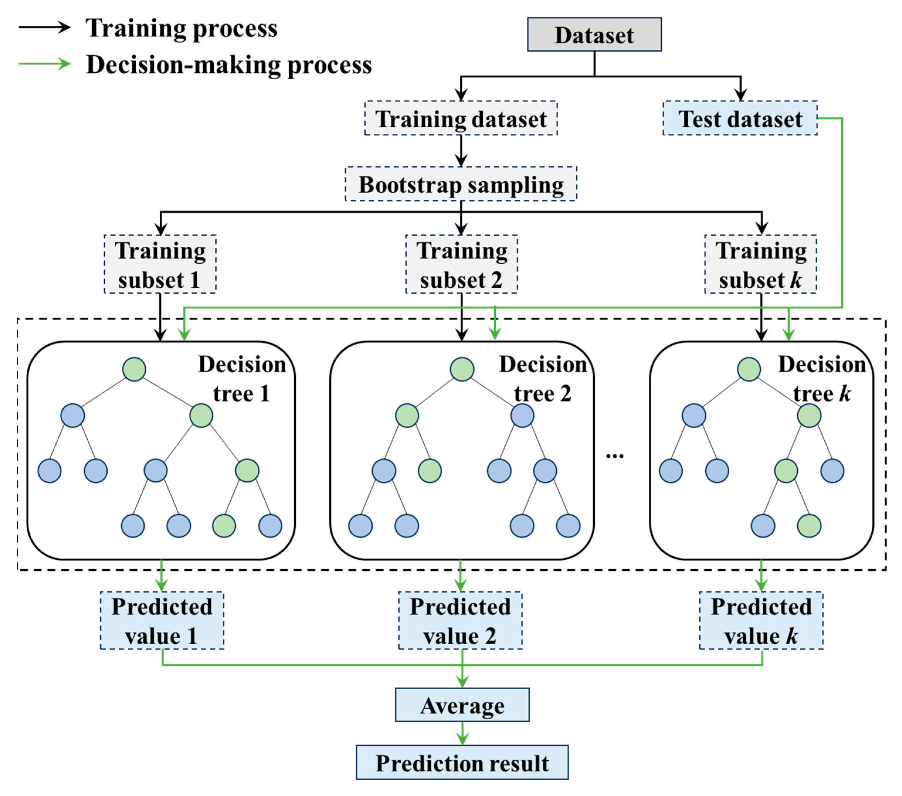
- Random forest (RF)
- (4)
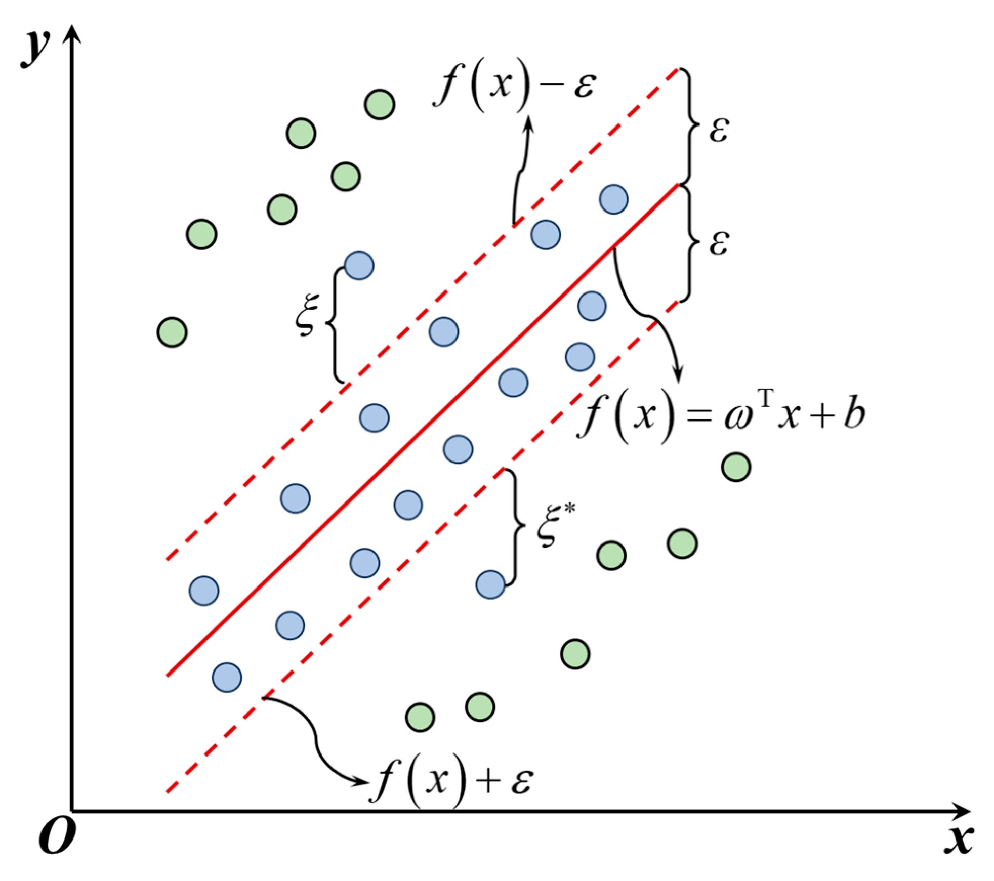
- Support vector regression (SVR)
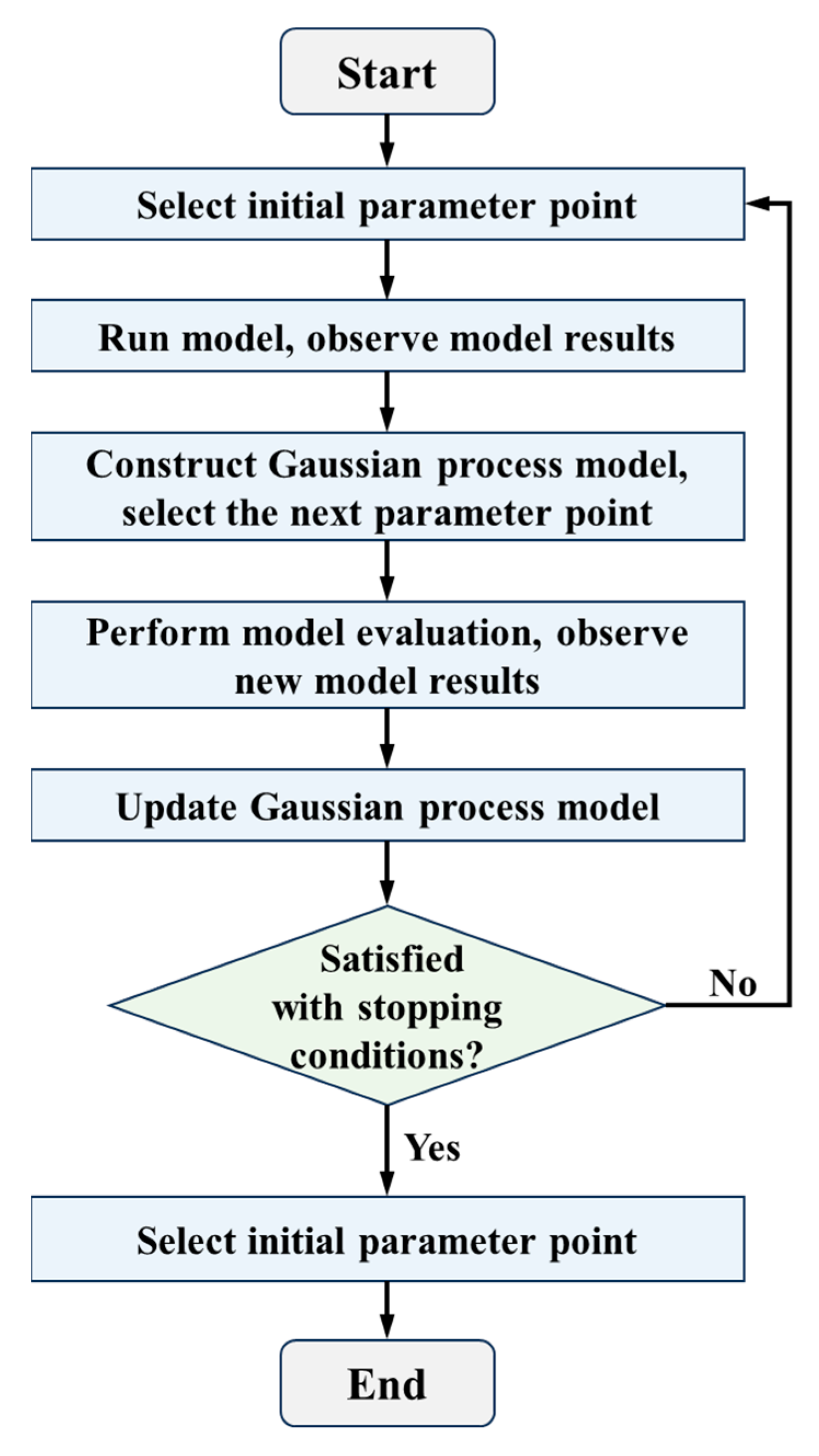
3.3.2. Hyperparameter Optimization
4. Results and Discussion
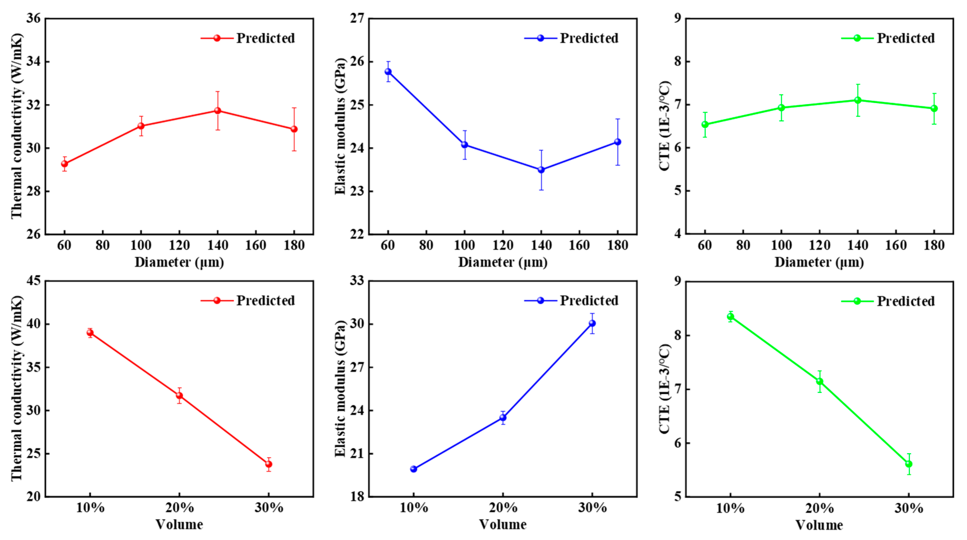
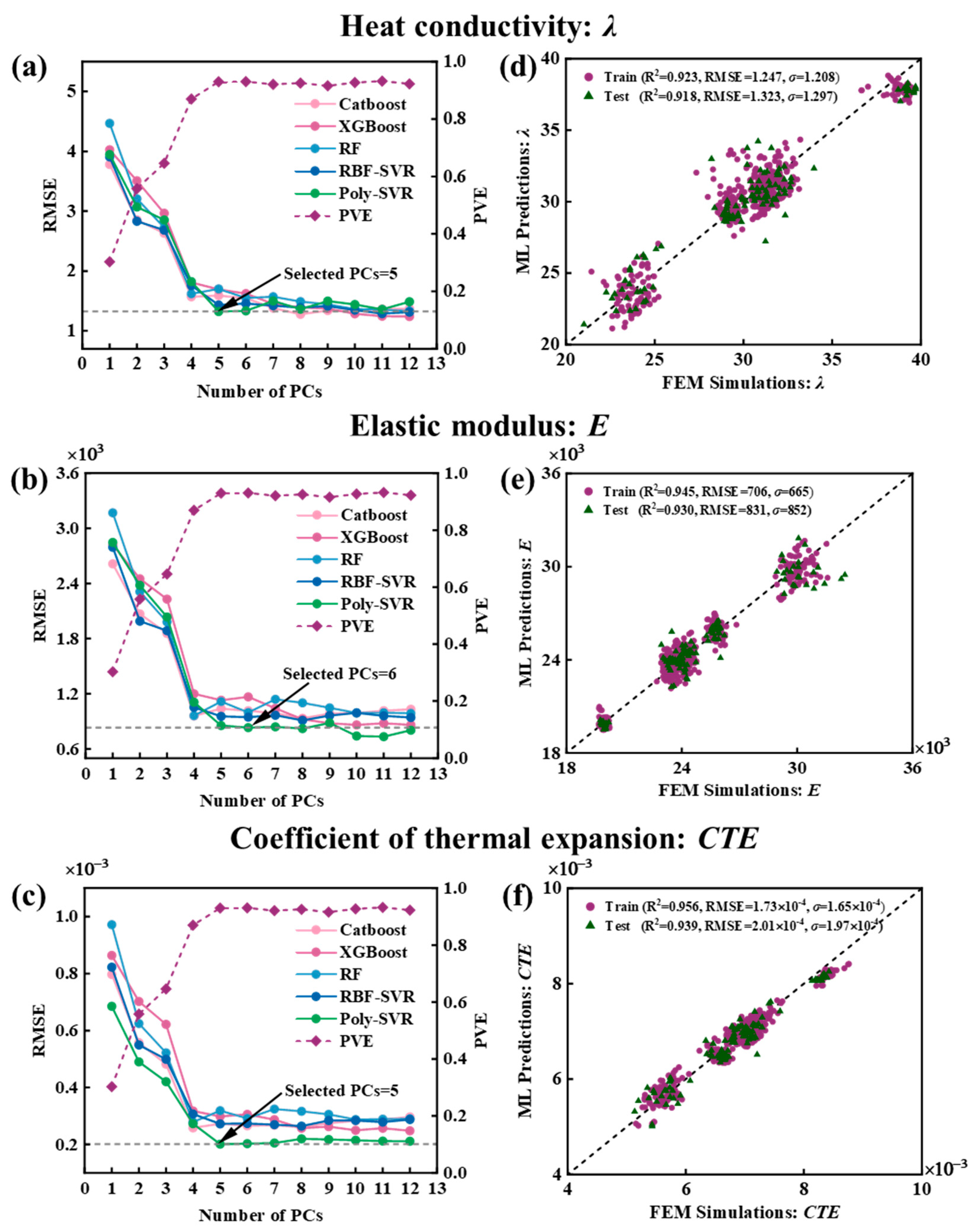
4.1. Extraction and Validation of SP Linkages
4.2. Discussion
5. Conclusions
Author Contributions
Funding
Institutional Review Board Statement
Informed Consent Statement
Data Availability Statement
Conflicts of Interest
References
- Miracle, D.B. Metal matrix composites–From science to technological significance. Compos. Sci. Technol. 2005, 65, 2526–2540. [Google Scholar] [CrossRef]
- Rajak, D.K.; Pagar, D.D.; Kumar, R.; Pruncu, C.I. Recent progress of reinforcement materials: A comprehensive overview of composite materials. J. Mater. Res. Technol. 2019, 8, 6354–6374. [Google Scholar] [CrossRef]
- Lin, Z.; Su, Y.; Qiu, C.; Yang, J.; Chai, X.; Liu, X.; Ouyang, Q.; Zhang, D. Configuration effect and mechanical behavior of particle reinforced aluminum matrix composites. Scr. Mater. 2023, 224, 115135. [Google Scholar] [CrossRef]
- Chen, X.-H.; Yan, H. Solid–liquid interface dynamics during solidification of Al 7075–Al2O3np based metal matrix composites. Mater. Des. 2016, 94, 148–158. [Google Scholar] [CrossRef]
- Wang, D.; Shanthraj, P.; Springer, H.; Raabe, D. Particle-induced damage in Fe–TiB2 high stiffness metal matrix composite steels. Mater. Des. 2018, 160, 557–571. [Google Scholar] [CrossRef]
- Song, M.; Huang, B. Effects of particle size on the fracture toughness of SiCp/Al alloy metal matrix composites. Mater. Sci. Eng. A. 2008, 488, 601–607. [Google Scholar] [CrossRef]
- Rabiei, A.; Vendra, L.; Kishi, T. Fracture behavior of particle reinforced metal matrix composites. Compos. Part A Appl. Sci. Manuf. 2008, 39, 294–300. [Google Scholar] [CrossRef]
- Liu, Q.; Qi, F.; Wang, Q.; Ding, H.; Chu, K.; Liu, Y.; Li, C. The influence of particles size and its distribution on the degree of stress concentration in particulate reinforced metal matrix composites. Mater. Sci. Eng. A 2018, 731, 351–359. [Google Scholar] [CrossRef]
- Jarzabek, D.M.; Chmielewski, M.; Dulnik, J.; Strojny-Nedza, A. The influence of the particle size on the adhesion between ceramic particles and metal matrix in mmc composites. J. Mater. Eng. Perform. 2016, 25, 3139–3145. [Google Scholar] [CrossRef]
- Singh, M.K.; Gautam, R.K. Structural, mechanical, and electrical behavior of ceramic-reinforced copper metal matrix hybrid composites. J. Mater. Eng. Perform. 2019, 28, 886–899. [Google Scholar] [CrossRef]
- Jarząbek, D.M. The impact of weak interfacial bonding strength on mechanical properties of metal matrix–Ceramic reinforced composites. Compos. Struct. 2018, 201, 352–362. [Google Scholar] [CrossRef]
- Yan, Y.-F.; Kou, S.-Q.; Yang, H.-Y.; Shu, S.-L.; Lu, J.-B. Effect mechanism of mono-particles or hybrid-particles on the thermophysical characteristics and mechanical properties of Cu matrix composites. Ceram. Int. 2022, 48, 23033–23043. [Google Scholar] [CrossRef]
- Commisso, M.S.; Le Bourlot, C.; Bonnet, F.; Zanelatto, O.; Maire, E. Thermo-mechanical characterization of steel-based metal matrix composite reinforced with TiB2 particles using synchrotron X-ray diffraction. Materialia 2019, 6, 100311. [Google Scholar] [CrossRef]
- León-Patiño, C.A.; González-Esquivel, R.J.; Aguilar-Reyes, E.A. Thermophysical properties of Ni–20Cr metal matrix reinforced with TiC ceramic particles. MRS Adv. 2021, 6, 807–810. [Google Scholar] [CrossRef]
- Chen, S.; Hassanzadeh-Aghdam, M.K.; Ansari, R. An analytical model for elastic modulus calculation of SiC whisker-reinforced hybrid metal matrix nanocomposite containing SiC nanoparticles. J. Alloys Compd. 2018, 767, 632–641. [Google Scholar] [CrossRef]
- Hashin, Z.; Shtrikman, S. A variational approach to the theory of the elastic behaviour of multiphase materials. J. Mech. Phys. Solids 1963, 11, 127–140. [Google Scholar] [CrossRef]
- Brailsford, A.D.; Major, K.G. The thermal conductivity of aggregates of several phases, including porous materials. Br. J. Appl. Phys. 1964, 15, 313. [Google Scholar] [CrossRef]
- Khan, K.; Hajeri, F.; Khan, M. Analytical and numerical assessment of the effect of highly conductive inclusions distribution on the thermal conductivity of particulate composites. J. Compos. Mater. 2019, 53, 3499–3514. [Google Scholar] [CrossRef]
- Sideridis, E. The influence of particle distribution and interphase on the thermal expansion coefficient of particulate composites by the use of a new model. Compos. Interfaces 2016, 23, 231–254. [Google Scholar] [CrossRef]
- Madan, R.; Khobragade, P.; Mussada, E.K.; Singh, M.K.; Rangappa, S.M.; Njim, E.K.; Siengchin, S. A novel two-step finite element approach to estimate the thermo-mechanical properties of two-phase and three-phase hybrid composites. Compos. Commun. 2025, 53, 102213. [Google Scholar] [CrossRef]
- Ma, S.; Zhuang, X.; Wang, X. Particle distribution-dependent micromechanical simulation on mechanical properties and damage behaviors of particle reinforced metal matrix composites. J. Mater. Sci. 2021, 56, 6780–6798. [Google Scholar] [CrossRef]
- Zhang, J.; Ouyang, Q.; Guo, Q.; Li, Z.; Fan, G.; Su, Y.; Jiang, L.; Lavernia, E.J.; Schoenung, J.M.; Zhang, D. 3D Microstructure-based finite element modeling of deformation and fracture of SiCp/Al composites. Compos. Sci. Technol. 2016, 123, 1–9. [Google Scholar] [CrossRef]
- Haušild, P.; Kovářík, O.; Havlíková, K.; Thomasová, M. Young’s modulus of alumina particles reinforced metal-matrix composite. Defect Diffus. Forum. 2016, 368, 174–177. [Google Scholar] [CrossRef]
- Hua, Y.; Gu, L. Prediction of the thermomechanical behavior of particle-reinforced metal matrix composites. Compos. Part B Eng. 2013, 45, 1464–1470. [Google Scholar] [CrossRef]
- Li, M.; Zhang, H.; Li, S.; Zhu, W.; Ke, Y. Machine learning and materials informatics approaches for predicting transverse mechanical properties of unidirectional CFRP composites with microvoids. Mater. Des. 2022, 224, 111340. [Google Scholar] [CrossRef]
- de Pablo, J.J.; Jackson, N.E.; Webb, M.A.; Chen, L.-Q.; Moore, J.E.; Morgan, D.; Jacobs, R.; Pollock, T.; Schlom, D.G.; Toberer, E.S.; et al. New frontiers for the materials genome initiative. npj Comput. Mater. 2019, 5, 41. [Google Scholar] [CrossRef]
- Lin, Z.; Su, Y.; Yang, J.; Qiu, C.; Chai, X.; Liu, X.; Ouyang, Q.; Zhang, D. Configuration feature extraction and mechanical properties prediction of particle reinforced metal matrix composites. Compos. Commun. 2023, 42, 101688. [Google Scholar] [CrossRef]
- Agrawal, A.; Choudhary, A. Perspective: Materials informatics and big data: Realization of the “fourth paradigm” of science in materials science. APL Mater. 2016, 4, 053208. [Google Scholar] [CrossRef]
- Chen, C.-T.; Gu, G.X. Generative deep neural networks for inverse materials design using backpropagation and active learning. Adv. Sci. 2020, 7, 1902607. [Google Scholar] [CrossRef]
- Ramprasad, R.; Batra, R.; Pilania, G.; Mannodi-Kanakkithodi, A.; Kim, C. Machine learning in materials informatics: Recent applications and prospects. npj Comput. Mater. 2017, 3, 54. [Google Scholar] [CrossRef]
- Mallela, U.K.; Upadhyay, A. Buckling load prediction of laminated composite stiffened panels subjected to in-plane shear using artificial neural networks. Thin-Walled Struct. 2016, 102, 158–164. [Google Scholar] [CrossRef]
- Barbosa, A.; Upadhyaya, P.; Iype, E. Neural network for mechanical property estimation of multilayered laminate composite. Mater. Today Proc. 2020, 28, 982–985. [Google Scholar] [CrossRef]
- Ye, S.; Li, B.; Li, Q.; Zhao, H.-P.; Feng, X.-Q. Deep neural network method for predicting the mechanical properties of composites. Appl. Phys. Lett. 2019, 115, 161901. [Google Scholar] [CrossRef]
- Yang, Z.; Yabansu, Y.C.; Jha, D.; Liao, W.-K.; Choudhary, A.N.; Kalidindi, S.R.; Agrawal, A. Establishing structure-property localization linkages for elastic deformation of three-dimensional high contrast composites using deep learning approaches. Acta Mater. 2019, 166, 335–345. [Google Scholar] [CrossRef]
- Liu, Z.; Wu, C.T. Exploring the 3D architectures of deep material network in data-driven multiscale mechanics. J. Mech. Phys. Solids 2019, 127, 20–46. [Google Scholar] [CrossRef]
- Olfatbakhsh, T.; Milani, A.S. A highly interpretable materials informatics approach for predicting microstructure-property relationship in fabric composites. Compos. Sci. Technol. 2022, 217, 109080. [Google Scholar] [CrossRef]
- Swaminathan, S.; Ghosh, S. Statistically equivalent representative volume elements for unidirectional composite microstructures: Part II-With interfacial debonding. J. Compos. Mater. 2006, 40, 605–621. [Google Scholar] [CrossRef]
- Feng, J.; Teng, Q.; He, X.; Wu, X. Accelerating multi-point statistics reconstruction method for porous media via deep learning. Acta Mater. 2018, 159, 296–308. [Google Scholar] [CrossRef]
- Qu, S.; Dai, Y.; Zhang, D.; Li, Q.; Chou, T.-W.; Lyu, W. Carbon nanotube film based multifunctional composite materials: An overview. Funct. Compos. Struct. 2020, 2, 022002. [Google Scholar] [CrossRef]
- Cecen, A.; Yabansu, Y.C.; Kalidindi, S.R. A new framework for rotationally invariant two-point spatial correlations in microstructure datasets. Acta Mater. 2018, 158, 53–64. [Google Scholar] [CrossRef]
- Cecen, A.; Fast, T.; Kalidindi, S.R. Versatile algorithms for the computation of 2-point spatial correlations in quantifying material structure. Integr. Mater. Manuf. Innov. 2016, 5, 1–15. [Google Scholar] [CrossRef]
- Hu, X.; Li, J.; Wang, Z.; Wang, J. A microstructure-informatic strategy for Vickers hardness forecast of austenitic steels from experimental data. Mater. Des. 2021, 201, 109497. [Google Scholar] [CrossRef]
- Jiang, M.; Hu, X.; Li, J.; Wang, Z.; Wang, J. An interface-oriented data-driven scheme applying into eutectic patterns evolution. Mater. Des. 2022, 223, 111222. [Google Scholar] [CrossRef]
- Zhao, Y.; Altschuh, P.; Santoki, J.; Griem, L.; Tosato, G.; Selzer, M.; Koeppe, A.; Nestler, B. Characterization of porous membranes using artificial neural networks. Acta Mater. 2023, 253, 118922. [Google Scholar] [CrossRef]
- Yi, Y.; Wang, L.; Chen, Z. Adaptive global kernel interval SVR-based machine learning for accelerated dielectric constant prediction of polymer-based dielectric energy storage. Renew. Energy 2021, 176, 81–88. [Google Scholar] [CrossRef]
- Qu, D.; Zheng, W.; Wang, B.; Wu, B.; Cao, H.; Yi, H. Nondestructive acquisition of the micro-mechanical properties of high-speed-dry milled micro-thin walled structures based on surface traits. Chin. J. Aeronaut. 2021, 34, 438–451. [Google Scholar] [CrossRef]
- Mann, A.; Kalidindi, S.R. Development of a robust CNN model for capturing microstructure-property linkages and building property closures supporting material design. Front. Mater. 2022, 9, 851085. [Google Scholar] [CrossRef]
- Yang, Z.; Yabansu, Y.C.; Al-Bahrani, R.; Liao, W.-k.; Choudhary, A.N.; Kalidindi, S.R.; Agrawal, A. Deep learning approaches for mining structure-property linkages in high contrast composites from simulation datasets. Comput. Mater. Sci. 2018, 151, 278–287. [Google Scholar] [CrossRef]
- Dong, X.; Shin, Y. Multi-scale modeling of thermal conductivity of SiC-reinforced aluminum metal matrix composite. J. Compos. Mater. 2017, 51, 3941–3953. [Google Scholar] [CrossRef]
- Kanit, T.; Forest, S.; Galliet, I.; Mounoury, V.; Jeulin, D. Determination of the size of the representative volume element for random composites: Statistical and numerical approach. Int. J. Solids Struct. 2003, 40, 3647–3679. [Google Scholar] [CrossRef]
- Luo, Y. An accuracy comparison of micromechanics models of particulate composites against microstructure-free finite element modeling. Materials 2022, 15, 4021. [Google Scholar] [CrossRef]
- van der Sluis, O.; Schreurs, P.J.G.; Brekelmans, W.A.M.; Meijer, H.E.H. Overall behaviour of heterogeneous elastoviscoplastic materials: Effect of microstructural modelling. Mech. Mater. 2000, 32, 449–462. [Google Scholar] [CrossRef]
- MacDonald, P.E.; Thompson, L.B. MATPRO: Version 09. A Handbook of Materials Properties for Use in the Analysis of Light Water Reactor Fuel Rod Behavior; U.S. Department of Energy Office of Scientific and Technical Information: Oak Ridge, TN, USA, 1976; p. 01.
- Hagrman, D.L.; Reymann, G.A. MATPRO-Version 11: A Handbook of Materials Properties for Use in the Analysis of Light Water Reactor Fuel Rod Behavior; U.S. Department of Energy Office of Scientific and Technical Information: Oak Ridge, TN, USA, 1979; p. 01.
- Kalidindi, S.B. Hierarchical Materials Informatics: Novel Analytics for Materials Data; Butterworth-Heinemann: Oxford, UK, 2015; pp. 1–219. [Google Scholar]
- Steinmetz, P.; Yabansu, Y.C.; Hötzer, J.; Jainta, M.; Nestler, B.; Kalidindi, S.R. Analytics for microstructure datasets produced by phase-field simulations. Acta Mater. 2016, 103, 192–203. [Google Scholar] [CrossRef]
- Fan, Y.S.; Yang, X.G.; Shi, D.Q.; Han, S.W.; Li, S.L. A quantitative role of rafting on low cycle fatigue behaviour of a directionally solidified Ni-based superalloy through a cross-correlated image processing method. Int. J. Fatigue 2020, 131, 105305. [Google Scholar] [CrossRef]
- Niezgoda, S.R.; Yabansu, Y.C.; Kalidindi, S.R. Understanding and visualizing microstructure and microstructure variance as a stochastic process. Acta Mater. 2011, 59, 6387–6400. [Google Scholar] [CrossRef]
- Choudhury, A.; Yabansu, Y.C.; Kalidindi, S.R.; Dennstedt, A. Quantification and classification of microstructures in ternary eutectic alloys using 2-point spatial correlations and principal component analyses. Acta Mater. 2016, 110, 131–141. [Google Scholar] [CrossRef]
- Altschuh, P.; Yabansu, Y.C.; Hötzer, J.; Selzer, M.; Nestler, B.; Kalidindi, S.R. Data science approaches for microstructure quantification and feature identification in porous membranes. J. Membr. Sci. 2017, 540, 88–97. [Google Scholar] [CrossRef]
- Yabansu, Y.C.; Steinmetz, P.; Hötzer, J.; Kalidindi, S.R.; Nestler, B. Extraction of reduced-order process-structure linkages from phase-field simulations. Acta Mater. 2017, 124, 182–194. [Google Scholar] [CrossRef]
- Niezgoda, S.R.; Kanjarla, A.K.; Kalidindi, S.R. Novel microstructure quantification framework for databasing, visualization, and analysis of microstructure data. Integr. Mater. Manuf. Innov. 2013, 2, 54–80. [Google Scholar] [CrossRef]
- Hao, W.; Shi, D.; Liu, C.; Fan, Y.; Yang, X.; Tan, L.; Zhang, B. A novel microstructure-informed machine learning framework for mechanical property evaluation of SiCf/Ti composites. J. Mater. Res. Technol. 2024, 28, 420–433. [Google Scholar] [CrossRef]
- Liu, X.; Liu, T.; Feng, P. Long-term performance prediction framework based on XGBoost decision tree for pultruded FRP composites exposed to water, humidity and alkaline solution. Compos. Struct. 2022, 284, 115184. [Google Scholar] [CrossRef]
- Huang, X.; Liu, W.; Guo, Q.; Tan, J. Prediction method for the dynamic response of expressway lateritic soil subgrades on the basis of Bayesian optimization CatBoost. Soil Dyn. Earthq. Eng. 2024, 186, 108943. [Google Scholar] [CrossRef]
- Breiman, L. Random Forests. Mach. Learn. 2001, 45, 5–32. [Google Scholar] [CrossRef]
- Wu, J.; Chen, X.-Y.; Zhang, H.; Xiong, L.-D.; Lei, H.; Deng, S.-H. Hyperparameter optimization for machine learning models based on Bayesian optimization. J. Electron. Sci. Technol. 2019, 17, 26–40. [Google Scholar]
- Bergstra, J.; Bengio, Y. Random search for hyper-parameter optimization. J. Mach. Learn. Res. 2012, 13, 281–305. [Google Scholar]
- Escherová, J.; Krbata, M.; Kohutiar, M.; Barényi, I.; Chochlíková, H.; Eckert, M.; Jus, M.; Majerský, J.; Janík, R.; Dubcová, P. The Influence of Q & T Heat Treatment on the Change of Tribological Properties of Powder Tool Steels ASP2017, ASP2055 and Their Comparison with Steel X153CrMoV12. Materials 2024, 17, 974. [Google Scholar] [CrossRef]


| Material | Density (kg/m3) | Thermal Conductivity W/(m·K) | Coefficient of Thermal Expansion (°C−1) | Elastic Modulus (MPa) | Poisson’s Ratio |
|---|---|---|---|---|---|
| UO2 | 10,600 | 2.3026 | 1.54 × 10⁻⁵ | 168,137 | 0.316 |
| Zr | 6550 | 47.4328 | 8.95 × 10⁻³ | 15,150 | 0.34 |
| Interface | 9790 | 11.3289 | 1.80 × 10⁻³ | 137,540 | 0.3208 |
| Machine Learning Model | Hyperparameter Settings |
|---|---|
| Poly-SVR | C ∈ [0.1, 100], epsilon ∈ [0.01, 0.5], degree ∈ [2, 5], coef0 ∈ [0, 1] |
| RBF-SVR | C ∈ [0.1, 100], epsilon ∈ [0.01, 0.5], gamma ∈ [0.01, 0.1, 1] |
| RF | n_estimators ∈ [10, 100], max_depth ∈ [3, 10], min_samples_split ∈ [2, 20], min_samples_leaf ∈ [1, 20] |
| XGBoost | n_estimators ∈ [10, 100], max_depth ∈ [3, 10], learning_rate ∈ [0.01, 0.5], subsample ∈ [0.6, 1], colsample_bytree ∈ [1, 20] |
| CatBoost | Iterations ∈ [10, 100], depth ∈ [3, 10], learning_rate ∈ [0.01, 0.5], l2_leaf_reg ∈ [1, 10], subsample ∈ [0.6, 1], colsample_bylevel ∈ [0.6, 1] |
| Property | Truncation | Data Volume | No. RVEs | Training RMSE | Test RMSE | Training R2 | Test R2 |
|---|---|---|---|---|---|---|---|
| Thermal conductivity | 0 | 1,436,592 | 600 | 1.292 | 1.681 | 0.918 | 0.867 |
| 96 | 750,000 | 600 | 1.247 | 1.323 | 0.923 | 0.918 | |
| 96 | 750,000 | 300 | 1.182 | 1.227 | 0.930 | 0.935 | |
| 146 | 480,000 | 600 | 1.231 | 1.379 | 0.925 | 0.911 | |
| Elastic modulus | 0 | 1,436,592 | 600 | 701.795 | 1156.328 | 0.946 | 0.865 |
| 96 | 750,000 | 600 | 706.179 | 830.8523 | 0.945 | 0.930 | |
| 96 | 750,000 | 300 | 696.629 | 810.255 | 0.948 | 0.929 | |
| 146 | 480,000 | 600 | 731.614 | 892.195 | 0.941 | 0.920 | |
| Coefficient of thermal expansion | 0 | 1,436,592 | 600 | 0.000229 | 0.000327 | 0.951 | 0.897 |
| 96 | 750,000 | 600 | 0.000216 | 0.000252 | 0.956 | 0.939 | |
| 96 | 750,000 | 300 | 0.000291 | 0.000326 | 0.918 | 0.905 | |
| 146 | 480,000 | 600 | 0.000228 | 0.000251 | 0.951 | 0.939 |
Disclaimer/Publisher’s Note: The statements, opinions and data contained in all publications are solely those of the individual author(s) and contributor(s) and not of MDPI and/or the editor(s). MDPI and/or the editor(s) disclaim responsibility for any injury to people or property resulting from any ideas, methods, instructions or products referred to in the content. |
© 2025 by the authors. Licensee MDPI, Basel, Switzerland. This article is an open access article distributed under the terms and conditions of the Creative Commons Attribution (CC BY) license (https://creativecommons.org/licenses/by/4.0/).
Share and Cite
Xie, R.; Li, G.; Cao, P.; Tan, Z.; Wang, J. Modeling the Structure–Property Linkages Between the Microstructure and Thermodynamic Properties of Ceramic Particle-Reinforced Metal Matrix Composites Using a Materials Informatics Approach. Materials 2025, 18, 2294. https://doi.org/10.3390/ma18102294
Xie R, Li G, Cao P, Tan Z, Wang J. Modeling the Structure–Property Linkages Between the Microstructure and Thermodynamic Properties of Ceramic Particle-Reinforced Metal Matrix Composites Using a Materials Informatics Approach. Materials. 2025; 18(10):2294. https://doi.org/10.3390/ma18102294
Chicago/Turabian StyleXie, Rui, Geng Li, Peng Cao, Zhifei Tan, and Jianru Wang. 2025. "Modeling the Structure–Property Linkages Between the Microstructure and Thermodynamic Properties of Ceramic Particle-Reinforced Metal Matrix Composites Using a Materials Informatics Approach" Materials 18, no. 10: 2294. https://doi.org/10.3390/ma18102294
APA StyleXie, R., Li, G., Cao, P., Tan, Z., & Wang, J. (2025). Modeling the Structure–Property Linkages Between the Microstructure and Thermodynamic Properties of Ceramic Particle-Reinforced Metal Matrix Composites Using a Materials Informatics Approach. Materials, 18(10), 2294. https://doi.org/10.3390/ma18102294