
Additive Manufacturing of Composite Polymers: Thermomechanical FEA and Experimental Study


Abstract
1. Introduction
2. Materials and Methods
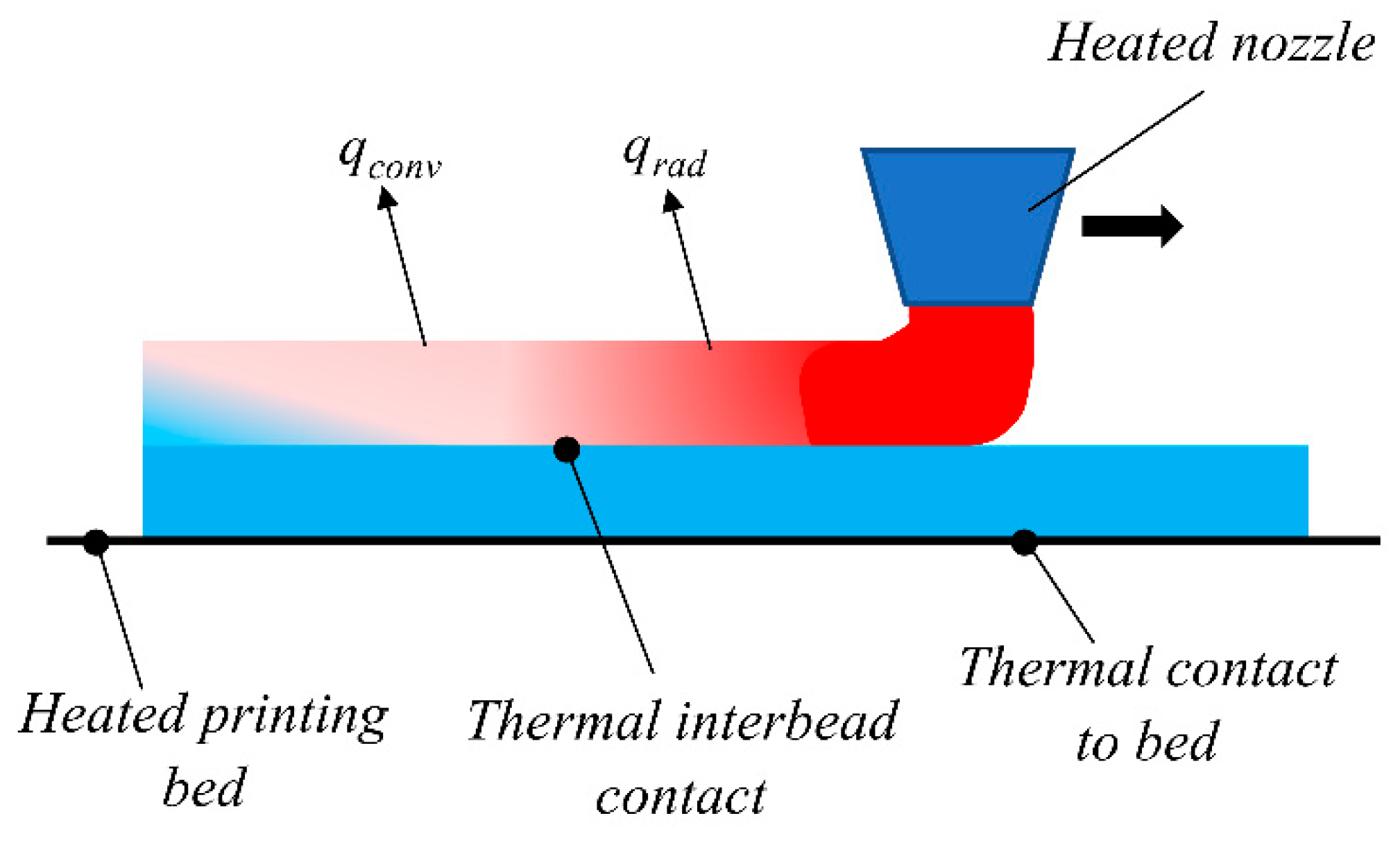
2.1. Thermal Analysis
2.2. Polymer Crystallization Kinetics
2.3. Viscoelastic Model of Orthotropic Materials
2.4. Determination of the Model Parameter
2.5. Anisotropic Shrinkage
3. Finite Element Simulation Technique
3.1. FEA-User Subroutines
3.1.1. UMATHT
3.1.2. UEPACTIVATIONVOL
3.1.3. ORIENT
3.1.4. UEXTERNALDB
3.1.5. UMAT
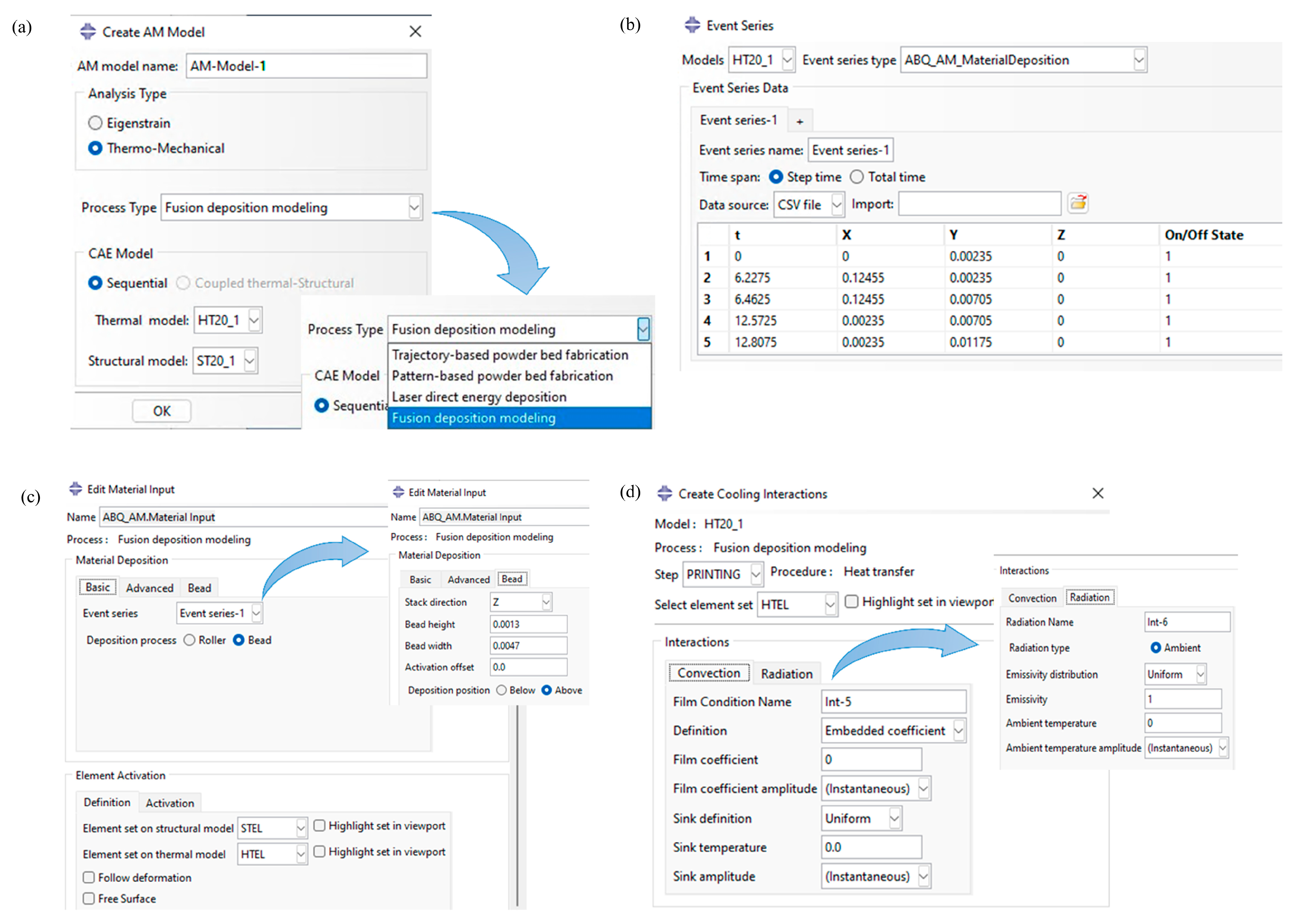
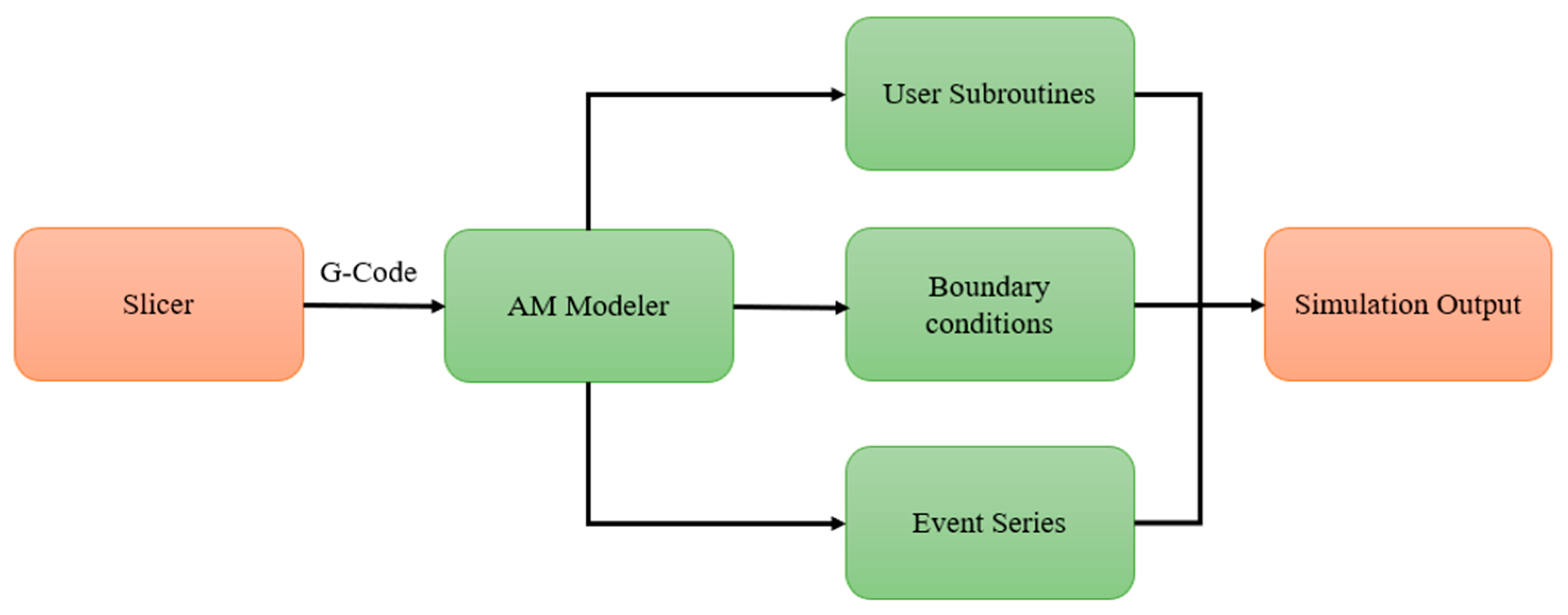
3.2. FEA-AM Modeler
4. Verification and Validation of FE Simulation Techniques
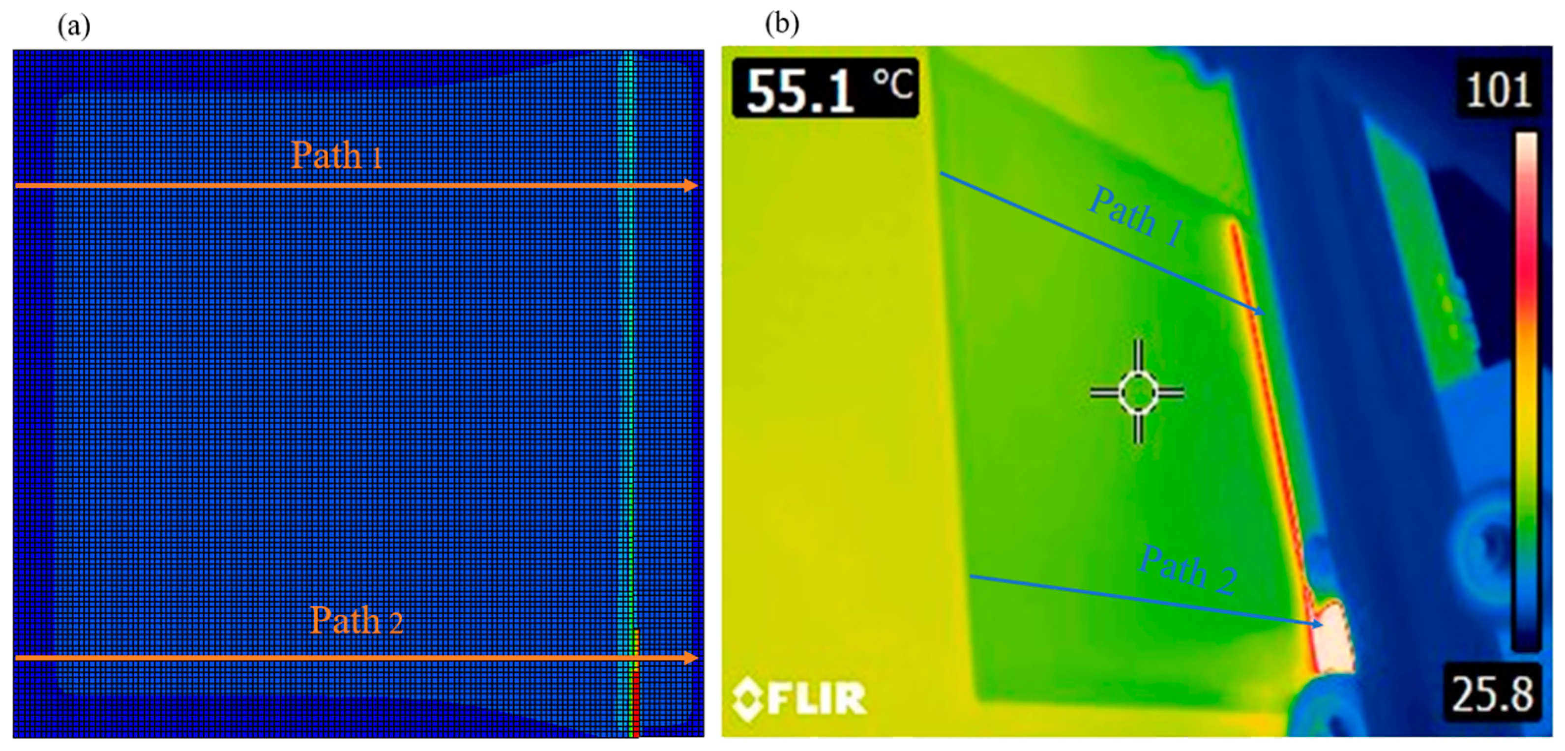
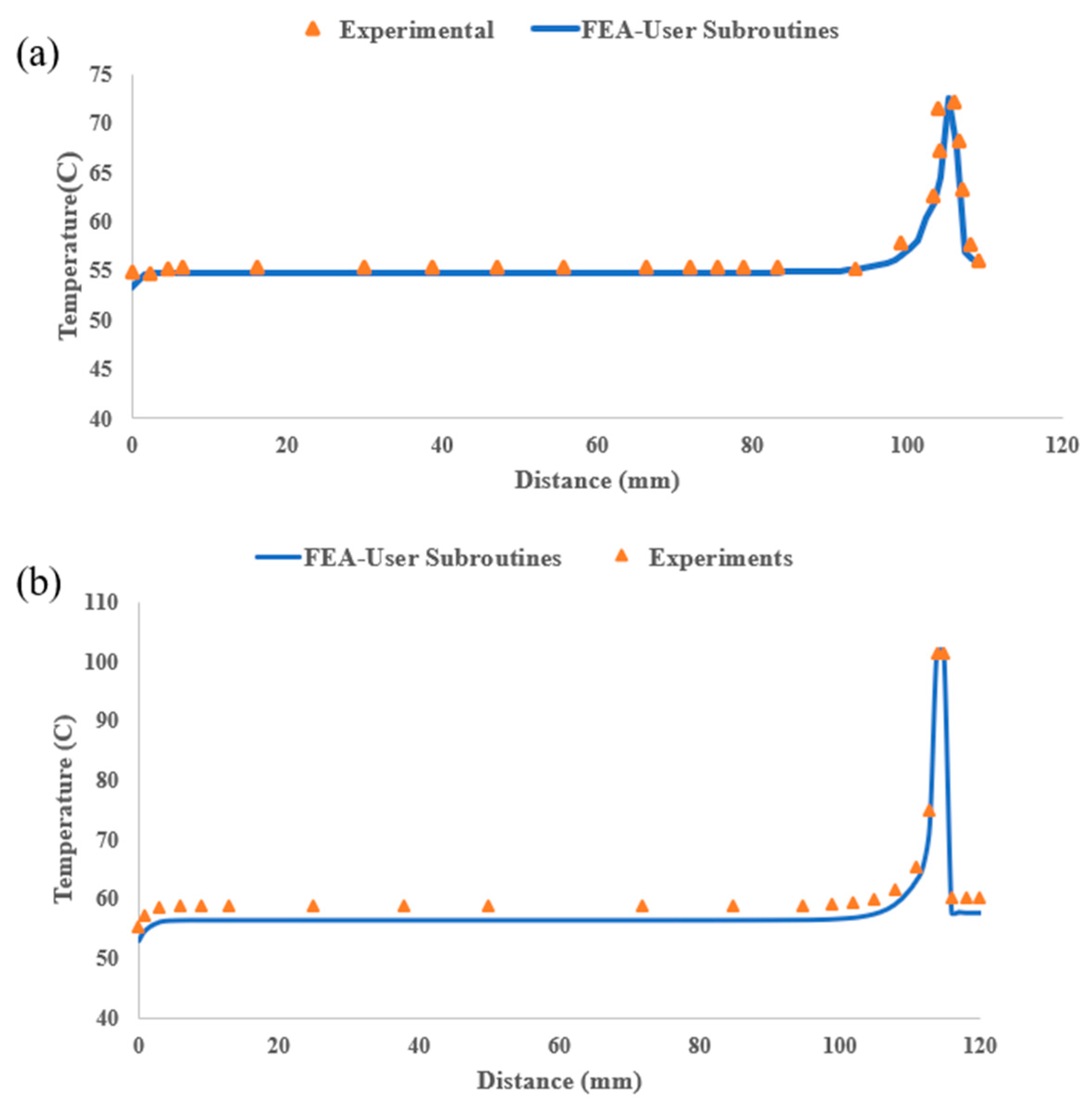
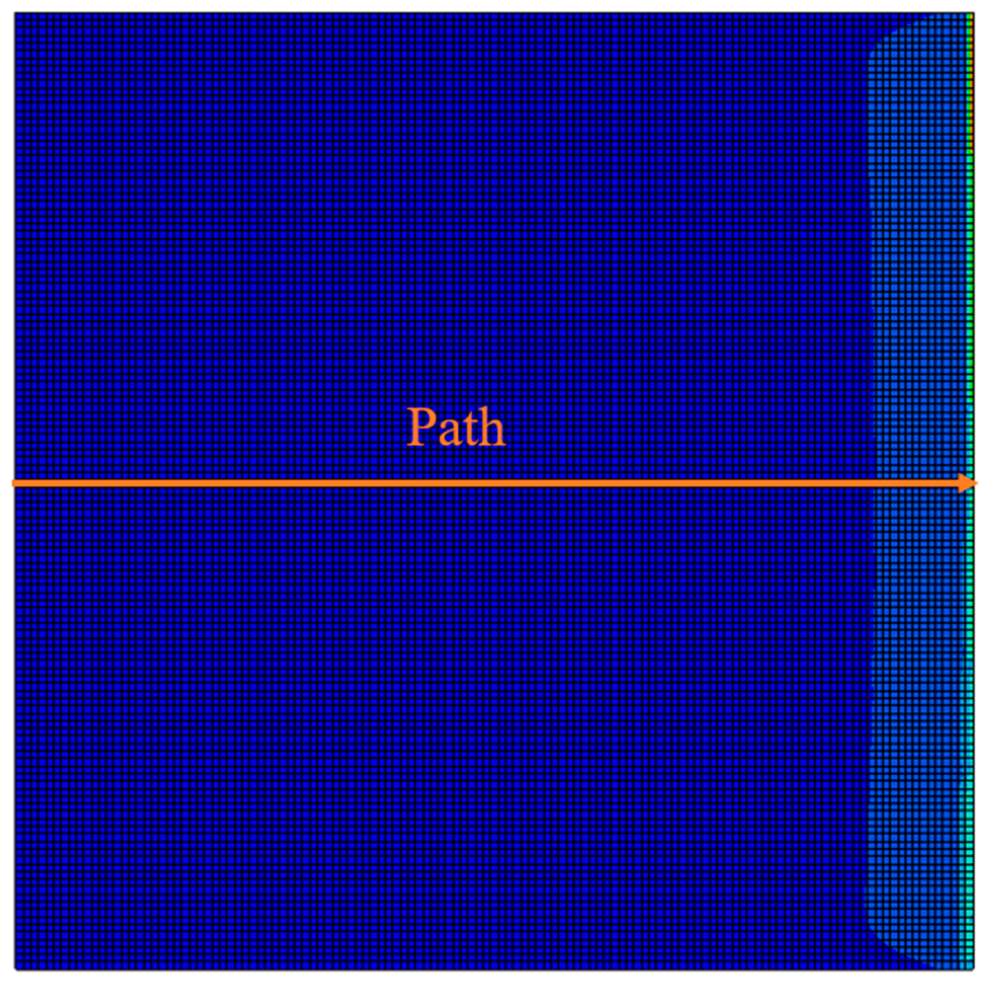
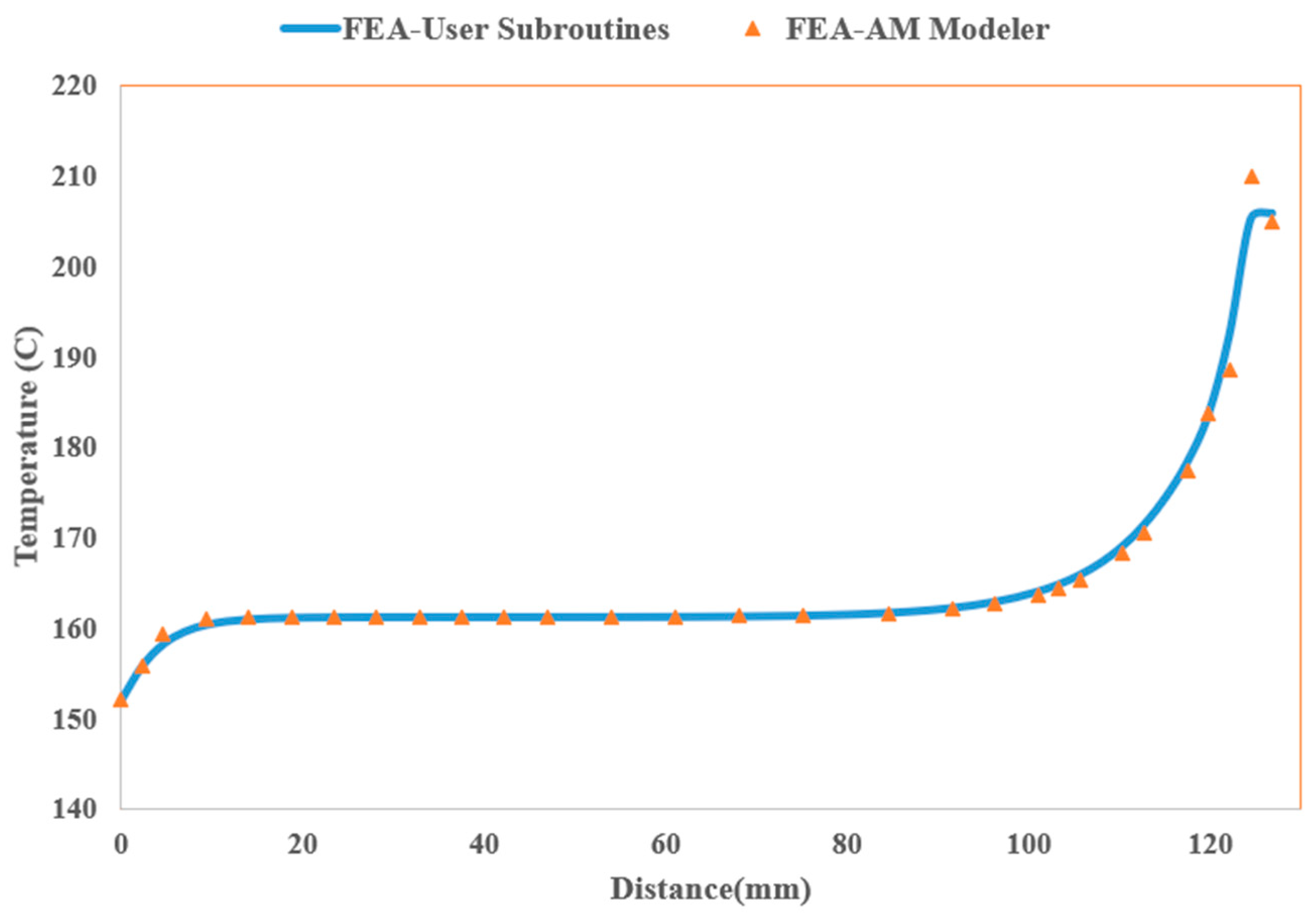
4.1. Thermal Analysis
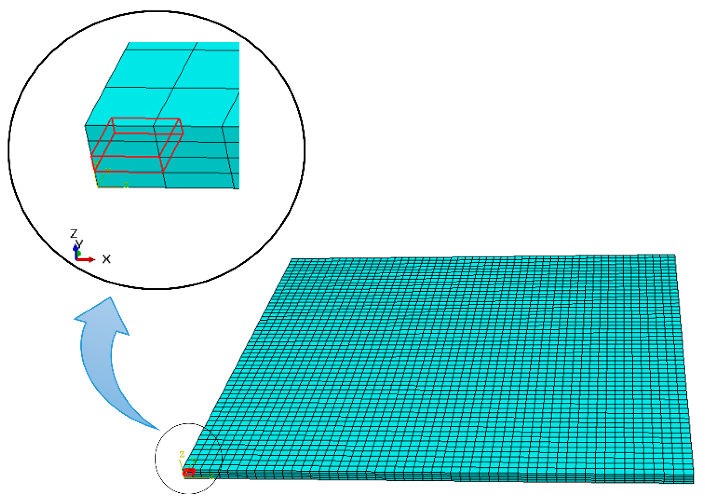
4.1.1. FE Simulation Model
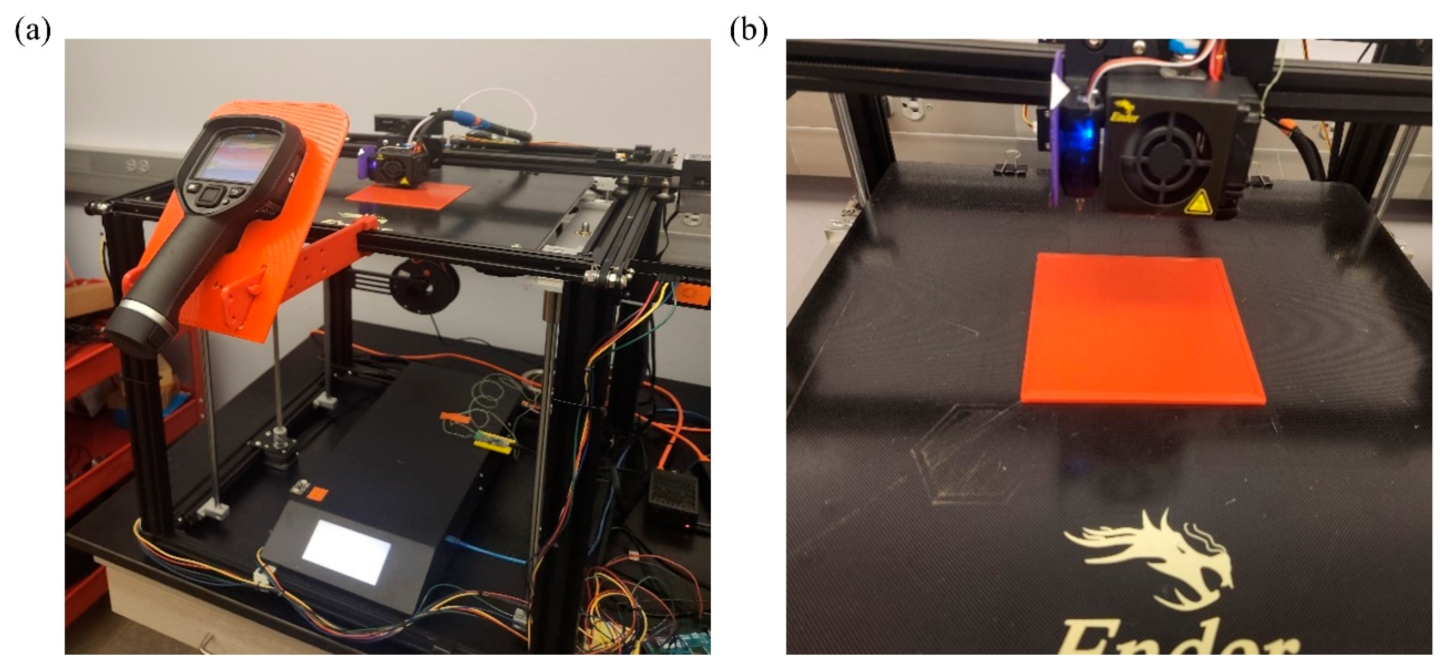
4.1.2. Experimental Verification
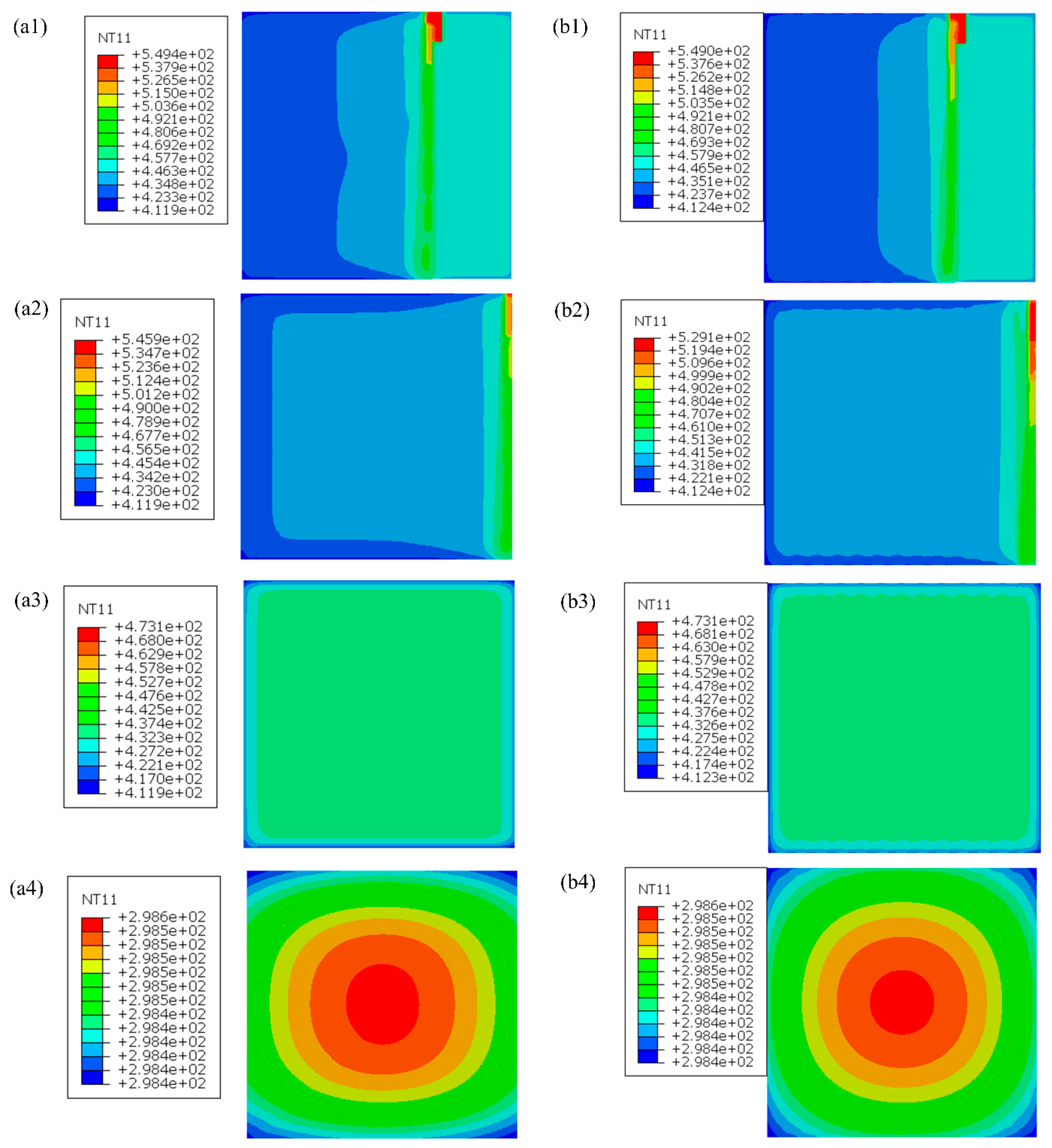
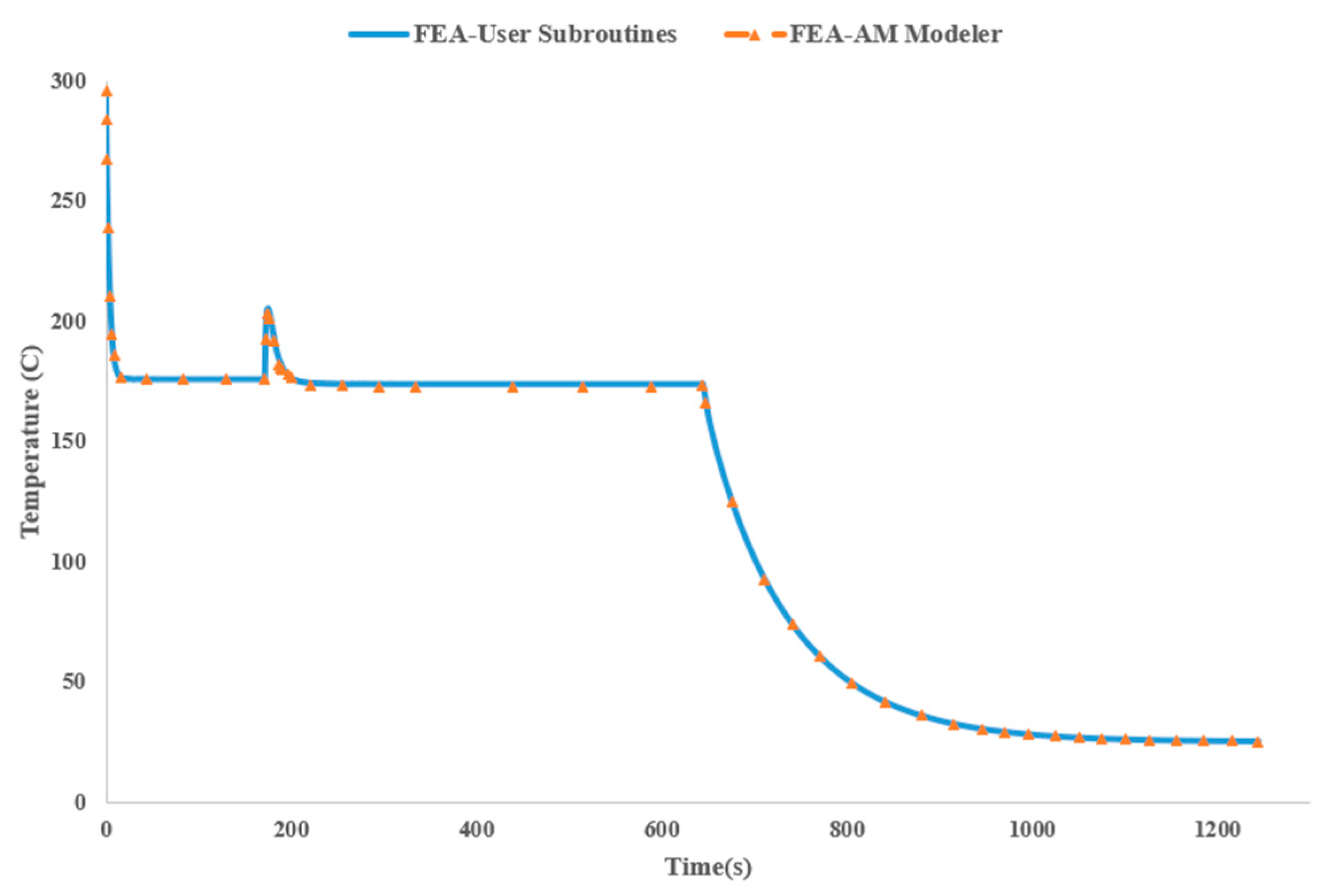
4.1.3. Verification of FEA-AM Modeler
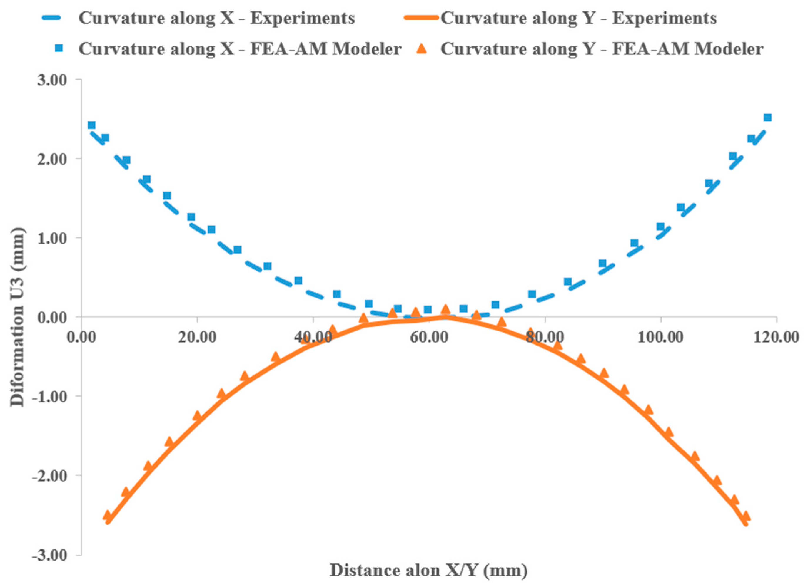
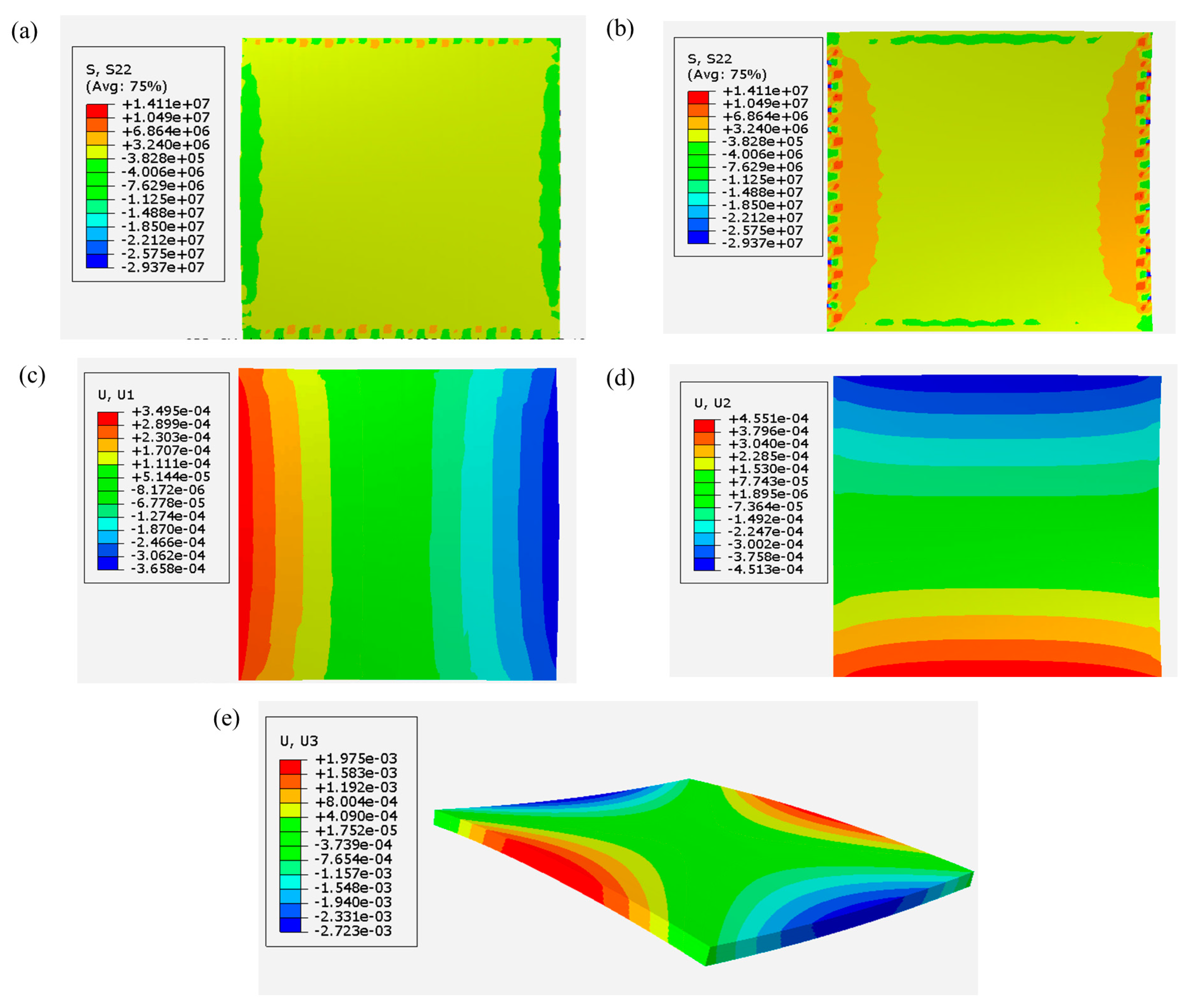
4.2. Mechanical Analysis
4.2.1. FE Simulation Model
4.2.2. Verification of FE Simulation
4.2.3. Residual Stresses and Distortion
5. Conclusions
Author Contributions
Funding
Institutional Review Board Statement
Informed Consent Statement
Data Availability Statement
Conflicts of Interest
References
- Mohamed, O.A.; Masood, S.H.; Bhowmik, J.L. Optimization of fused deposition modeling process parameters: A review of current research and future prospects. Adv. Manuf. 2015, 3, 42–53. [Google Scholar] [CrossRef]
- Gibson, I.; Rosen, D.W.; Stucker, B.; Khorasani, M.; Rosen, D.; Stucker, B.; Khorasani, M. Additive Manufacturing Technologies; Springer: Berlin/Heidelberg, Germany, 2021; Volume 17. [Google Scholar]
- Chua, C.K.; Leong, K.F.; Lim, C.S. Rapid Prototyping: Principles and Applications (with Companion CD-ROM); World Scientific Publishing Company: Singapore, 2010. [Google Scholar]
- Upcraft, S.; Fletcher, R. The rapid prototyping technologies. Assem. Autom. 2003, 23, 318–330. [Google Scholar] [CrossRef]
- Mansour, S.; Hague, R. Impact of rapid manufacturing on design for manufacture for injection moulding. Proc. Inst. Mech. Eng. Part B J. Eng. Manuf. 2003, 217, 453–461. [Google Scholar] [CrossRef]
- Hague, R.; Dickens, P.; Hopkinson, N. Rapid Manufacturing: An Industrial Revolution for the Digital Age; John Wiley & Sons: Hoboken, NJ, USA, 2006. [Google Scholar]
- Thavornyutikarn, B.; Chantarapanich, N.; Sitthiseripratip, K.; Thouas, G.A.; Chen, Q. Bone tissue engineering scaffolding: Computer-aided scaffolding techniques. Prog. Biomater. 2014, 3, 61–102. [Google Scholar] [CrossRef]
- Ahn, S.H.; Montero, M.; Odell, D.; Roundy, S.; Wright, P.K. Anisotropic material properties of fused deposition modeling ABS. Rapid Prototyp. J. 2002, 8, 248–257. [Google Scholar] [CrossRef]
- An, N.; Yang, G.; Yang, K.; Wang, J.; Li, M.; Zhou, J. Implementation of Abaqus user subroutines and plugin for thermal analysis of powder-bed electron-beam-melting additive manufacturing process. Mater. Today Commun. 2021, 27, 102307. [Google Scholar] [CrossRef]
- Brenken, B.; Barocio, E.; Favaloro, A.; Kunc, V.; Pipes, R.B. Fused filament fabrication of fiber-reinforced polymers: A review. Addit. Manuf. 2018, 21, 1–16. [Google Scholar] [CrossRef]
- Yao, T.; Ye, J.; Deng, Z.; Zhang, K.; Ma, Y.; Ouyang, H. Tensile failure strength and separation angle of FDM 3D printing PLA material: Experimental and theoretical analyses. Compos. Part B Eng. 2020, 188, 107894. [Google Scholar] [CrossRef]
- Attoye, S.O. A Study of Fused Deposition Modeling (FDM) 3-D Printing Using Mechanical Testing and Thermography; Purdue University: West Lafayette, IN, USA, 2018. [Google Scholar]
- Tangri, M. Predicting Mechanical Behavior of 3D Printed Structures Using Mechanics of Composites and Fracture; The University of Texas at Arlington: Arlington, TX, USA, 2018. [Google Scholar]
- Prabhakar, P.; Sames, W.J.; Dehoff, R.; Babu, S.S. Computational modeling of residual stress formation during the electron beam melting process for Inconel 718. Addit. Manuf. 2015, 7, 83–91. [Google Scholar] [CrossRef]
- Samy, A.A.; Golbang, A.; Harkin-Jones, E.; Archer, E.; McIlhagger, A. Prediction of part distortion in Fused Deposition Modelling (FDM) of semi-crystalline polymers via COMSOL: Effect of printing conditions. CIRP J. Manuf. Sci. Technol. 2021, 33, 443–453. [Google Scholar] [CrossRef]
- Xia, H.; Lu, J.; Tryggvason, G. A numerical study of the effect of viscoelastic stresses in fused filament fabrication. Comput. Methods Appl. Mech. Eng. 2019, 346, 242–259. [Google Scholar] [CrossRef]
- Han, P.; Zhang, S.; Tofangchi, A.; Hsu, K. Relaxation of residual stress in fused filament fabrication part with in-process laser heating. Procedia Manuf. 2021, 53, 466–471. [Google Scholar] [CrossRef]
- Fischer, J.M. Handbook of Molded Part Shrinkage and Warpage, 2nd ed.; William Andrew: Norwich, NY, USA, 2012. [Google Scholar]
- Hertle, S.; Drexler, M.; Drummer, D. Additive manufacturing of poly(propylene) by means of melt extrusion. Macromol. Mater. Eng. 2016, 301, 1482–1493. [Google Scholar] [CrossRef]
- Ruan, C.; Guo, L.; Liang, K.; Li, W. Computer modeling and simulation for 3D crystallization of polymers. II. Non-isothermal case. Polym. Plast. Technol. Eng. 2012, 51, 816–822. [Google Scholar] [CrossRef]
- Wang, J.; Papadopoulos, P. Coupled thermomechanical analysis of fused deposition using the finite element method. Finite Elem. Anal. Des. 2021, 197, 103607. [Google Scholar] [CrossRef]
- Zhou, Y.; Nyberg, T.; Xiong, G.; Liu, D. Temperature analysis in the fused deposition modeling process. In Proceedings of the 2016 3rd International Conference on Information Science and Control Engineering (ICISCE), Beijing, China, 8–10 July 2016. [Google Scholar]
- Zhou, X.; Hsieh, S.-J.; Sun, Y. Experimental and numerical investigation of the thermal behaviour of polylactic acid during the fused deposition process. Virtual Phys. Prototyp. 2017, 12, 221–233. [Google Scholar] [CrossRef]
- Costa, S.; Duarte, F.; Covas, J. Thermal conditions affecting heat transfer in FDM/FFE: A contribution towards the numerical modelling of the process. Virtual Phys. Prototyp. 2015, 10, 35–46. [Google Scholar] [CrossRef]
- Favaloro, A.J.; Brenken, B.; Barocio, E.; Pipes, R.B. Simulation of polymeric composites additive manufacturing using Abaqus. Sci. Age Exp. 2017, 103–114. [Google Scholar]
- Zhang, Y.; Chou, Y. Three-dimensional finite element analysis simulations of the fused deposition modelling process. Proc. Inst. Mech. Eng. Part B J. Eng. Manuf. 2006, 220, 1663–1671. [Google Scholar] [CrossRef]
- Yang, H.; Zhang, S. Numerical simulation of temperature field and stress field in fused deposition modeling. J. Mech. Sci. Technol. 2018, 32, 3337–3344. [Google Scholar] [CrossRef]
- Charlon, S.; Le Boterff, J.; Soulestin, J. Fused filament fabrication of polypropylene: Influcen of the bead temperature on adhesion and porosity. Addit. Manuf. 2021, 38, 101838. [Google Scholar] [CrossRef]
- Hussein, A.; Hao, L.; Yan, C.; Everson, R. Finite Element Simulation of the Temperature and Stress Fields in Single Layers Built without-Support in Selective Laser Melting. Mater. Des. 2013, 52, 638–647. [Google Scholar] [CrossRef]
- Cattenone, A.; Alaimo, G.; Auricchio, F. Finite Element Analysis of Additive Manufacturing Based on Fused Deposition Modeling: Distortions Prediction and Comparison With Experimental Data. J. Manuf. Sci. Eng. 2019, 141, 011010-17. [Google Scholar] [CrossRef]
- Brenken, B. Extrusion Deposition Additive Manufacturing of Fiber Reinforced Semi-Crystalline Polymers; Purdue University: West Lafayette, IN, USA, 2017. [Google Scholar]
- Velisaris, C.N.; Seferis, J.C. Crystallization kinetics of polyetheretherketone (peek) matrices. Polym. Eng. Sci. 1986, 26, 1574–1581. [Google Scholar] [CrossRef]
- Chapman, T.J.; Gillespie, J.W.; Pipes, R.B.; Månson, J.-A.E.; Seferis, J.C. Prediction of Process-Induced Residual Stresses in Thermoplastic Composites. J. Compos. Mater. 1990, 24, 616–643. [Google Scholar] [CrossRef]
- Behseresht, S.; Mehdizadeh, M. Mode I&II SIFs for semi-elliptical crack in a cylinder wrapped with a composite layer. In Proceedings of the 28th Annual International Conference of Iranian Society of Mechanical Engineers-ISME2020, Tehran, Iran, 27–29 May 2020. [Google Scholar]
- Behseresht, S.; Mehdizadeh, M. Stress intensity factor interaction between two semi-elliptical cracks in thin-walled cylinder. In Proceedings of the 28th Annual International Conference of Iranian Society of Mechanical Engineers-ISME2020, Tehran, Iran, 27–29 May 2020. [Google Scholar]
- Taylor, R.L.; Pister, K.S.; Goudreau, G.L. Thermomechanical Analysis of Viscoelastic Solids. Int. J. Numer. Methods Eng. 1970, 2, 45–59. [Google Scholar] [CrossRef]
- Sunderland, P.; Yu, W.; Månson, J.A. A thermoviscoelastic analysis of processinduced internal stresses in thermoplastic matrix composites. Polym. Compos. 2001, 22, 579–592. [Google Scholar] [CrossRef]
- Brenken, B.; Barocio, E.; Favaloro, A.; Kunc, V.; Pipes, R.B. Development and validation of extrusion deposition additive manufacturing process simulations. Addit. Manuf. 2019, 25, 218–226. [Google Scholar] [CrossRef]
- Zmeskal, O.; Marackova, L.; Lapcikova, T.; Mencik, P.; Prikryl, R. Thermal properties of samples prepared from polylactic acid by 3D printing. AIP Conf. Proc. 2020, 2305, 020022. [Google Scholar]


| Parameter | Value |
|---|---|
| Print speed | 20 mm/s |
| Ambient temperature | 25 °C |
| emissivity | 0.97 |
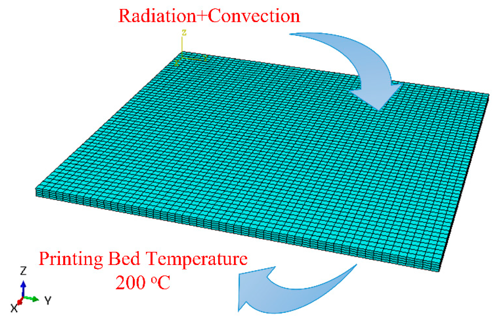
| Bed temperature | 200 °C |
| Number of elements | 11,664 |
| Convection film coefficient | 30 W/(mK) |
| Parameter | Value |
|---|---|
| Print speed | 20 mm/s |
| Layer height | 0.5 mm |
| Extrusion temperature | 210 °C |
| Bed temperature | 60 °C |
Disclaimer/Publisher’s Note: The statements, opinions and data contained in all publications are solely those of the individual author(s) and contributor(s) and not of MDPI and/or the editor(s). MDPI and/or the editor(s) disclaim responsibility for any injury to people or property resulting from any ideas, methods, instructions or products referred to in the content. |
© 2024 by the authors. Licensee MDPI, Basel, Switzerland. This article is an open access article distributed under the terms and conditions of the Creative Commons Attribution (CC BY) license (https://creativecommons.org/licenses/by/4.0/).
Share and Cite
Behseresht, S.; Park, Y.H. Additive Manufacturing of Composite Polymers: Thermomechanical FEA and Experimental Study. Materials 2024, 17, 1912. https://doi.org/10.3390/ma17081912
Behseresht S, Park YH. Additive Manufacturing of Composite Polymers: Thermomechanical FEA and Experimental Study. Materials. 2024; 17(8):1912. https://doi.org/10.3390/ma17081912
Chicago/Turabian StyleBehseresht, Saeed, and Young Ho Park. 2024. "Additive Manufacturing of Composite Polymers: Thermomechanical FEA and Experimental Study" Materials 17, no. 8: 1912. https://doi.org/10.3390/ma17081912
APA StyleBehseresht, S., & Park, Y. H. (2024). Additive Manufacturing of Composite Polymers: Thermomechanical FEA and Experimental Study. Materials, 17(8), 1912. https://doi.org/10.3390/ma17081912