

Atomic Diffusivities of Yttrium, Titanium and Oxygen Calculated by Ab Initio Molecular Dynamics in Molten 316L Oxide-Dispersion-Strengthened Steel Fabricated via Additive Manufacturing

 , , , ,
  ,
,  and
and
Abstract
1. Introduction
2. Methodology
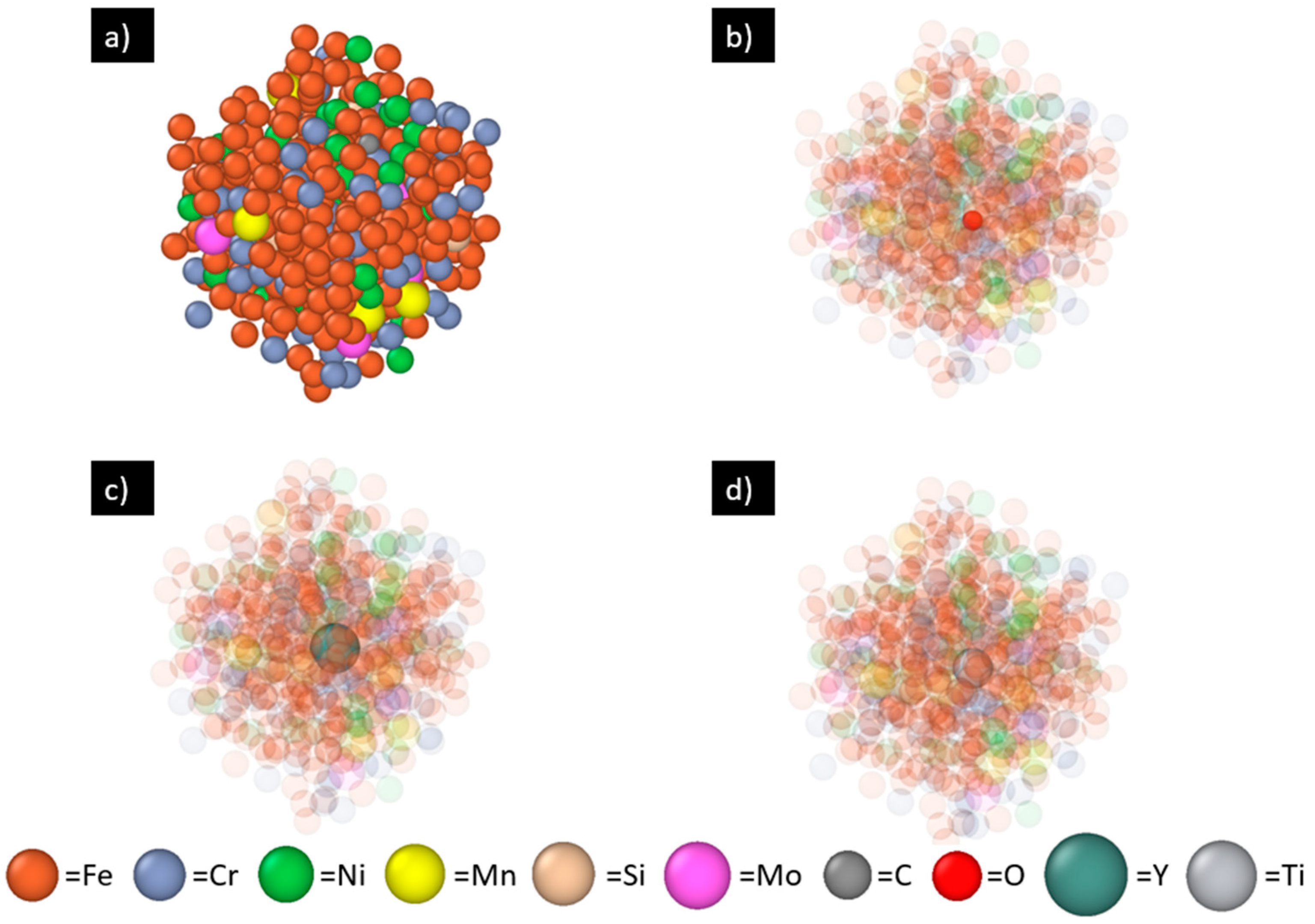
2.1. VASP Setup
2.1.1. The Machine Learning Force Field (MLFF)
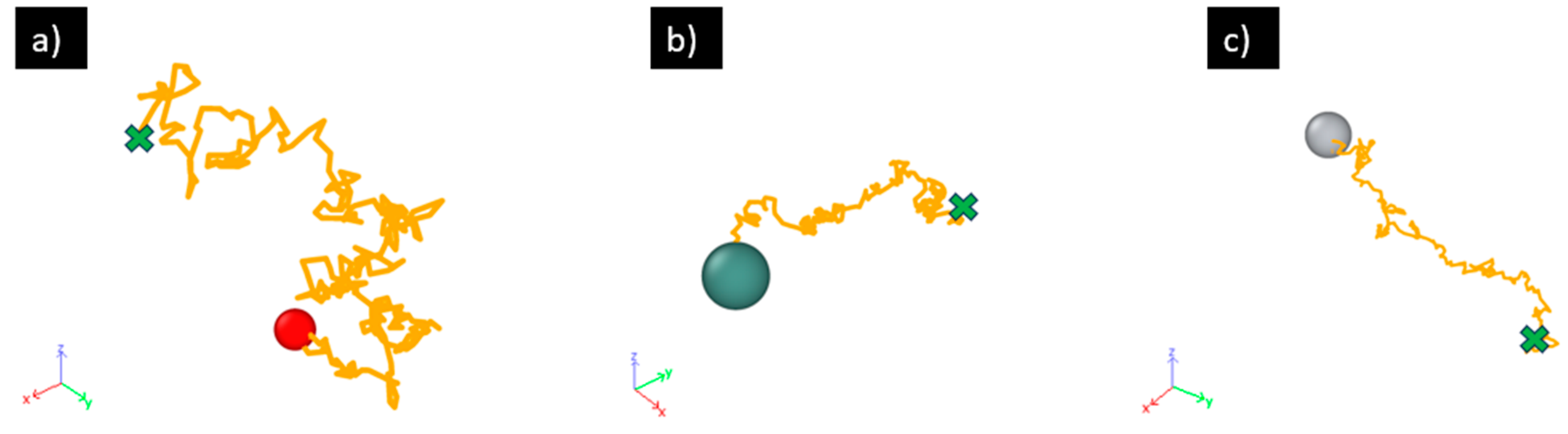
2.1.2. Diffusion Simulation
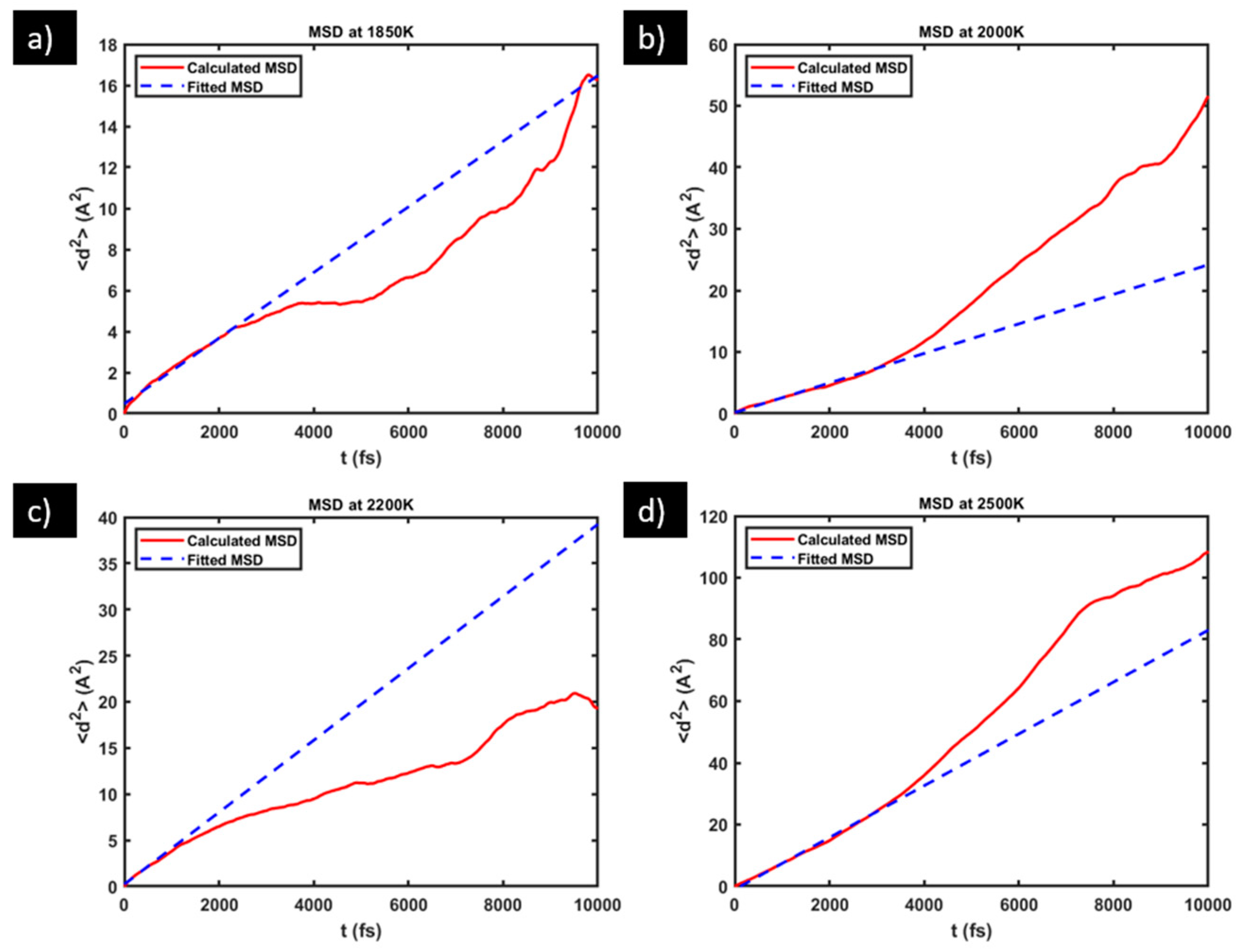
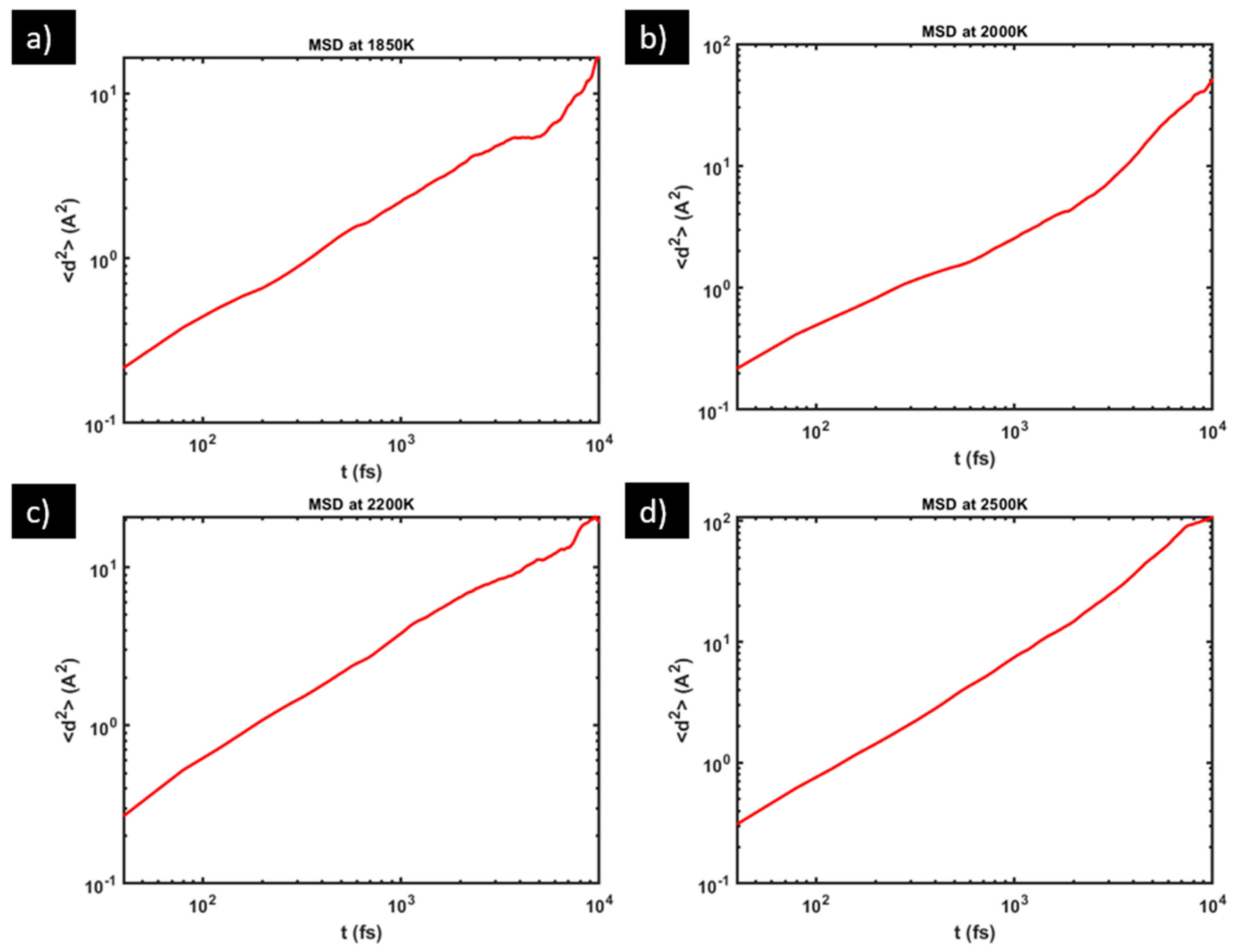
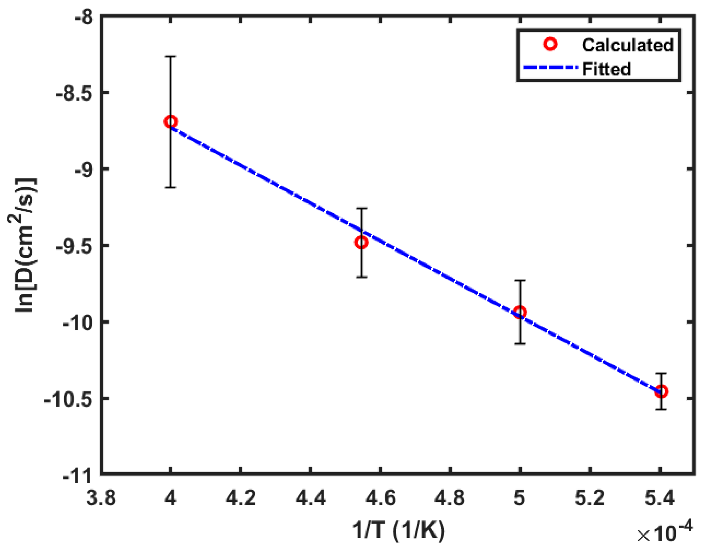
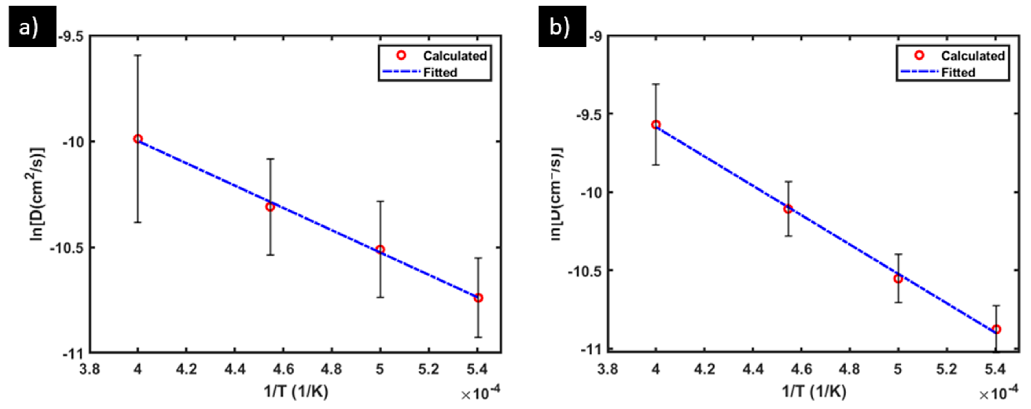
2.2. Diffusivity Calculation
3. Results and Discussion
3.1. Diffusivity of Oxygen
3.2. Diffusivities of Yttrium and Titanium
3.3. Discussion
4. Conclusions
Supplementary Materials
Author Contributions
Funding
Data Availability Statement
Acknowledgments
Conflicts of Interest
References
- Odette, G.R. On the status and prospects for nanostructured ferritic alloys for nuclear fission and fusion application with emphasis on the underlying science. Scr. Mater. 2018, 143, 142–148. [Google Scholar] [CrossRef]
- Zinkle, S.J.; Boutard, J.L.; Hoelzer, D.T.; Kimura, A.; Lindau, R.; Odette, G.R.; Rieth, M.; Tan, L.; Tanigawa, H. Development of next generation tempered and ODS reduced activation ferritic/martensitic steels for fusion energy applications. Nucl. Fusion. 2017, 57, 092005. [Google Scholar] [CrossRef]
- Zinkle, S.J.; Snead, L.L. Designing Radiation Resistance in Materials for Fusion Energy. Annu. Rev. Mater. Res. 2014, 44, 241–267. [Google Scholar] [CrossRef]
- Zinkle, S.J.; Busby, J.T. Structural materials for fission & fusion energy. Mater. Today 2009, 12, 12–19. [Google Scholar]
- Allen, T.; Busby, J.; Meyer, M.; Petti, D. Materials challenges for nuclear systems. Mater. Today 2010, 13, 14–23. [Google Scholar] [CrossRef]
- Certain, A.G.; Field, K.G.; Allen, T.R.; Miller, M.K.; Bentley, J.; Busby, J.T. Response of nanoclusters in a 9Cr ODS steel to 1 dpa, 525 °C proton irradiation. J. Nucl. Mater. 2010, 407, 2–9. [Google Scholar] [CrossRef]
- Allen, T.R.; Gan, J.; Cole, J.I.; Miller, M.K.; Busby, J.T.; Shutthanandan, S.; Thevuthasan, S. Radiation response of a 9 chromium oxide dispersion strengthened steel to heavy ion irradiation. J. Nucl. Mater. 2008, 375, 26–37. [Google Scholar] [CrossRef]
- Ghayoor, M.; Lee, K.J.; He, Y.J.; Chang, C.H.; Paul, B.K.; Pasebani, S. Selective laser melting of austenitic oxide dispersion strengthened steel: Processing, microstructural evolution and strengthening mechanisms. Mater. Sci. Eng. A 2020, 788, 139532. [Google Scholar] [CrossRef]
- Sridharan, N.; Dryepondt, S.N.; Field, K.G. Investigation of Laser Direct Energy Deposition for Production of ODS Alloys; No. ORNL/SPR-2018/983; M3NT-18OR020202072; Oak Ridge National Lab.: Oak Ridge, TN, USA, 2018. [Google Scholar]
- Doñate-Buendia, C.; Kürnsteiner, P.; Stern, F.; Wilms, M.B.; Streubel, R.; Kusoglu, I.M.; Tenkamp, J.; Bruder, E.; Pirch, N.; Barcikowski, S.; et al. Microstructure formation and mechanical properties of ODS steels built by laser additive manufacturing of nanoparticle coated iron-chromium powders. Acta Mater. 2021, 206, 116566. [Google Scholar] [CrossRef]
- Miao, Y.B.; Mo, K.; Zhou, Z.J.; Liu, X.; Lan, K.C.; Zhang, G.M.; Miller, M.K.; Powers, K.A.; Mei, Z.-G.; Park, J.-S.; et al. On the microstructure and strengthening mechanism in oxide dispersion-strengthened 316 steel: A coordinated electron microscopy, atom probe tomography and in situ synchrotron tensile investigation. Mater. Sci. Eng. A 2015, 639, 585–596. [Google Scholar] [CrossRef]
- Miao, Y.B.; Mo, K.; Cui, B.; Chen, W.Y.; Miller, M.K.; Powers, K.A.; McCreary, V.; Gross, D.; Almer, J.; Robertson, I.M.; et al. The interfacial orientation relationship of oxide nanoparticles in a hafnium-containing oxide dispersion-strengthened austenitic stainless steel. Mater. Charact. 2015, 101, 136–143. [Google Scholar] [CrossRef]
- Yan, X.L.; Zhang, X.; Wang, F.; Stockdale, T.; Dzenis, Y.; Nastasi, M.; Cui, B. Fabrication of ODS austenitic steels and CoCrFeNi high-entropy alloys by spark plasma sintering for nuclear energy applications. JOM 2019, 71, 2856–2867. [Google Scholar] [CrossRef]
- Ghayoor, M.; Mirzababaei, S.; Sittiho, A.; Charit, I.; Paul, B.K.; Pasebani, S. Thermal stability of additively manufactured austenitic 304L ODS alloy. J. Mater. Sci. Technol. 2021, 83, 208–218. [Google Scholar] [CrossRef]
- Mirzababaei, S.; Ghayoor, M.; Doyle, R.P.; Pasebani, S. In-situ manufacturing of ODS FeCrAlY alloy via laser powder bed fusion. Mater. Lett. 2021, 284, 129046. [Google Scholar] [CrossRef]
- Wang, Y.; Wang, B.B.; Luo, L.S.; Li, B.Q.; Liu, T.; Zhao, J.H.; Xu, B.B.; Wang, L.; Su, Y.; Guo, J.; et al. Laser-based powder bed fusion of pre-alloyed oxide dispersion strengthened steel containing yttrium. Addit. Manuf. 2022, 58, 103018. [Google Scholar] [CrossRef]
- Yang, S.; Xu, D.H.; Yan, D.Q.; Albert, M.; Pasebani, S. Additive Manufacturing of ODS Steels Using Powder Feedstock Atomized with Elemental Yttrium. In Proceedings of the 34th Annual International Solid Freeform Fabrication Symposium—An Additive Manufacturing Conference, Austin, TX, USA, 14–16 August 2023; pp. 1478–1488. [Google Scholar]
- Suresh, K.; Nagini, M.; Vijay, R.; Ramakrishna, M.; Gundakaram, R.C.; Reddy, A.V.; Sundararajan, G. Microstructural studies of oxide dispersion strengthened austenitic steels. Mater. Des. 2016, 110, 519–525. [Google Scholar] [CrossRef]
- García-Junceda, A.; Hernández-Mayoral, M.; Serrano, M. Influence of the microstructure on the tensile and impact properties of a 14Cr ODS steel bar. Mater. Sci. Eng. A 2012, 556, 696–703. [Google Scholar] [CrossRef]
- Miao, P.; Odette, G.R.; Yamamoto, T.; Alinger, M.; Klingensmith, D. Thermal stability of nano-structured ferritic alloy. J. Nucl. Mater. 2008, 377, 59–64. [Google Scholar] [CrossRef]
- Barnard, L.; Cunningham, N.; Odette, G.R.; Szlufarska, I.; Morgan, D. Thermodynamic and kinetic modeling of oxide precipitation in nanostructured ferritic alloys. Acta Mater. 2015, 91, 340–354. [Google Scholar] [CrossRef]
- Kawakami, M.; Goto, K.S. Oxygen Diffusivity in Molten Iron Determined by Oxygen Concentration Cell Technique at 1550 °C. Trans. Iron Steel Inst. Jpn. 1976, 16, 204–207. [Google Scholar] [CrossRef]
- Suzuki, K.; Mori, K. Diffusion of oxygen in molten iron. Tetsu--Hagané 1971, 57, 2219–2229. [Google Scholar] [CrossRef] [PubMed]
- Saito, T.; Kawai, Y.; Maruya, K.; Maki, M. Diffusion of some alloying elements in liquid iron. Sci. Rep. Res. Inst. Tohoku Univ. Ser. A Phys. Chem. Metall. 1959, 11, 401–410. [Google Scholar]
- Kubíček, P.; Pepřica, T. Diffusion in molten metals and melts: Application to diffusion in molten iron. Int. Met. Rev. 1983, 28, 131–157. [Google Scholar] [CrossRef]
- Mock, M.; Albe, K. Diffusion of yttrium in bcc-iron studied by kinetic Monte Carlo simulations. J. Nucl. Mater. 2017, 494, 157–164. [Google Scholar] [CrossRef]
- Gao, X.Y.; Ren, H.P.; Li, C.L.; Wang, H.Y.; Ji, Y.P.; Tan, H.J. First-principles calculations of rare earth (Y, La and Ce) diffusivities in bcc Fe. J. Alloys Compd. 2016, 663, 316–320. [Google Scholar] [CrossRef]
- Wang, X.; Faßbender, J.; Posselt, M. Mutual dependence of oxygen and vacancy diffusion in bcc Fe and dilute iron alloys. Phys. Rev. B 2020, 101, 174107. [Google Scholar] [CrossRef]
- Hepworth, M.T.; Smith, R.P.; Turkdogan, E.T. Permeability, solubility, and diffusivity of oxygen in bcc iron. AIME Met. Soc. Trans. 1966, 236, 1278–1283. [Google Scholar]
- Swisher, J.H.; Turkdogan, E.T. Solubility, permeability, and diffusivity of oxygen in solid iron. AIME Met. Soc. Trans. 1967, 239, 426–431. [Google Scholar]
- Klugkist, P.; Herzig, C. Tracer diffusion of titanium in α-iron. Phys. Status Solidi (A) 1995, 148, 413–421. [Google Scholar] [CrossRef]
- Shapovalov, V.P.; Kurasov, A.N. Diffusion of titanium in iron. Met. Sci. Heat. Treat. 1975, 17, 803–805. [Google Scholar] [CrossRef]
- Kresse, G. Ab-Initio Molekular Dynamik für Flüssige Metalle. Ph.D. Thesis, Technische University at Wien, Vienna, Austria, 1993. [Google Scholar]
- Kresse, G.; Furthmüller, J. Efficient iterative schemes for ab initio total-energy calculations using a plane-wave basis set. Phys. Rev. B 1996, 54, 11169. [Google Scholar] [CrossRef] [PubMed]
- Kresse, G.; Furthmüller, J. Efficiency of ab-initio total energy calculations for metals and semiconductors using a plane-wave basis set. Comput. Mater. Sci. 1996, 6, 15–50. [Google Scholar] [CrossRef]
- Kresse, G.; Hafner, J. Ab initio molecular dynamics for liquid metals. Phys. Rev. B 1993, 47, 558. [Google Scholar] [CrossRef]
- Kresse, G.; Joubert, D. From ultrasoft pseudopotentials to the projector augmented-wave method. Phys. Rev. B 1999, 59, 1758. [Google Scholar] [CrossRef]
- Perdew, J.P.; Burke, K.; Ernzerhof, M. Generalized gradient approximation made simple. Phys. Rev. Lett. 1996, 77, 3865. [Google Scholar] [CrossRef]
- Stukowski, A. Visualization and analysis of atomistic simulation data with OVITO—The Open Visualization Tool. Model. Simul. Mater. Sci. Eng. 2010, 18, 015012. [Google Scholar] [CrossRef]
- Periodic Table. Available online: https://ptable.com (accessed on 10 February 2024).


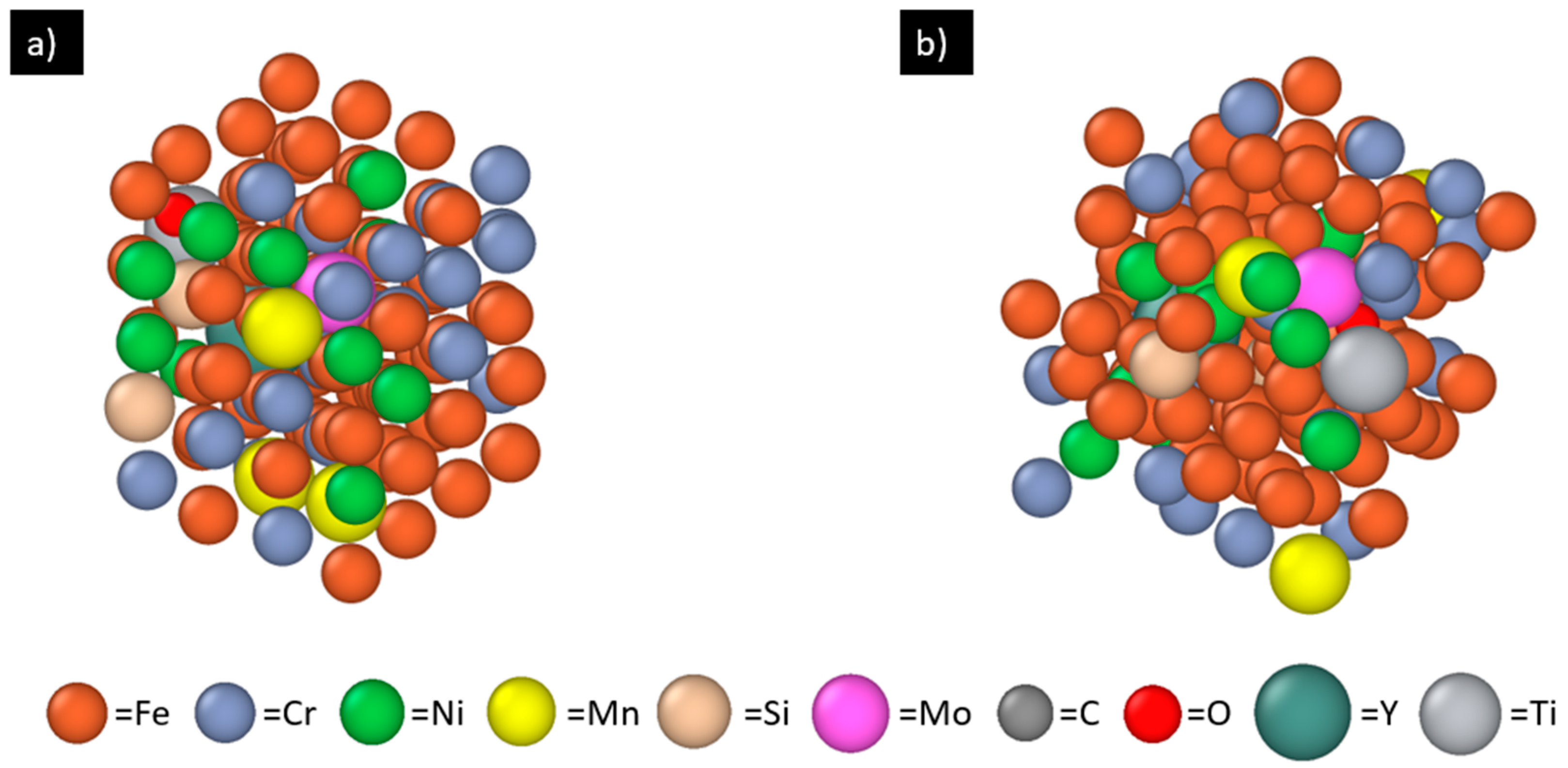
| Fe | Cr | Ni | Mn | Si | Mo | C | P | S | Total | |
|---|---|---|---|---|---|---|---|---|---|---|
| Nominal composition (at.%) | Bal | 17.90 | 9.33 | 1.99 | 1.46 | 1.15 | 0.36 | 0.08 | 0.05 | 100 |
| No. of atoms (for learning) | 86 | 23 | 12 | 3 | 2 | 1 | 1 | 0 | 0 | 128 |
| No. of atoms (for diffusion simulations) | 292 | 77 | 41 | 9 | 6 | 5 | 2 | 0 | 0 | 432 |
| T (K) | 1850 | 2000 | 2200 | 2500 |
|---|---|---|---|---|
| DS1 (10−5 cm2/s) | 2.71 | 3.93 | 6.51 | 12.7 |
| DS2 (10−5 cm2/s) | 2.67 | 5.93 | 9.85 | 27.4 |
| DS3 (10−5 cm2/s) | 3.28 | 4.79 | 6.87 | 13.5 |
| Average D (10−5 cm2/s) | 2.89 | 4.88 | 7.74 | 17.87 |
| T (K) | 1850 | 2000 | 2200 | 2500 |
|---|---|---|---|---|
| Ave. DY (10−5 cm2/s) | 2.19 | 2.77 | 3.39 | 4.85 |
| Ave. DTi (10−5 cm2/s) | 1.90 | 2.63 | 4.11 | 7.14 |
Disclaimer/Publisher’s Note: The statements, opinions and data contained in all publications are solely those of the individual author(s) and contributor(s) and not of MDPI and/or the editor(s). MDPI and/or the editor(s) disclaim responsibility for any injury to people or property resulting from any ideas, methods, instructions or products referred to in the content. |
© 2024 by the authors. Licensee MDPI, Basel, Switzerland. This article is an open access article distributed under the terms and conditions of the Creative Commons Attribution (CC BY) license (https://creativecommons.org/licenses/by/4.0/).
Share and Cite
Wang, Z.; Yang, S.; Lawson, S.B.; Doddapaneni, V.V.K.; Albert, M.; Sutton, B.; Chang, C.-H.; Pasebani, S.; Xu, D. Atomic Diffusivities of Yttrium, Titanium and Oxygen Calculated by Ab Initio Molecular Dynamics in Molten 316L Oxide-Dispersion-Strengthened Steel Fabricated via Additive Manufacturing. Materials 2024, 17, 1543. https://doi.org/10.3390/ma17071543
Wang Z, Yang S, Lawson SB, Doddapaneni VVK, Albert M, Sutton B, Chang C-H, Pasebani S, Xu D. Atomic Diffusivities of Yttrium, Titanium and Oxygen Calculated by Ab Initio Molecular Dynamics in Molten 316L Oxide-Dispersion-Strengthened Steel Fabricated via Additive Manufacturing. Materials. 2024; 17(7):1543. https://doi.org/10.3390/ma17071543
Chicago/Turabian StyleWang, Zhengming, Seongun Yang, Stephanie B. Lawson, V. Vinay K. Doddapaneni, Marc Albert, Benjamin Sutton, Chih-Hung Chang, Somayeh Pasebani, and Donghua Xu. 2024. "Atomic Diffusivities of Yttrium, Titanium and Oxygen Calculated by Ab Initio Molecular Dynamics in Molten 316L Oxide-Dispersion-Strengthened Steel Fabricated via Additive Manufacturing" Materials 17, no. 7: 1543. https://doi.org/10.3390/ma17071543
APA StyleWang, Z., Yang, S., Lawson, S. B., Doddapaneni, V. V. K., Albert, M., Sutton, B., Chang, C.-H., Pasebani, S., & Xu, D. (2024). Atomic Diffusivities of Yttrium, Titanium and Oxygen Calculated by Ab Initio Molecular Dynamics in Molten 316L Oxide-Dispersion-Strengthened Steel Fabricated via Additive Manufacturing. Materials, 17(7), 1543. https://doi.org/10.3390/ma17071543