Article

Derivation of Corrosion Depth Formula According to Corrosion Factors in District Heating Water through Regression Analysis

1
School of Advanced Materials Science and Engineering, Sungkyunkwan University, Suwon 16419, Republic of Korea
2
Plant Management and QC Division, Korea District Heating Corporation, Sungnam 13585, Republic of Korea
*
Author to whom correspondence should be addressed.
Materials 2023, 16(8), 3254; https://doi.org/10.3390/ma16083254
Submission received: 28 March 2023 / Revised: 17 April 2023 / Accepted: 19 April 2023 / Published: 20 April 2023
(This article belongs to the Special Issue Corrosion Prediction and Corrosion Protection)

Abstract

:
In order to predict the corrosion depth of a district heating pipeline, it is necessary to analyze various corrosion factors. In this study, the relationship between corrosion factors such as pH, dissolved oxygen, and operating time and corrosion depth was investigated using the Box–Behnken method within the response surface methodology. To accelerate the corrosion process, galvanostatic tests were conducted in synthetic district heating water. Subsequently, a multiple regression analysis was performed using the measured corrosion depth to derive a formula for predicting the corrosion depth as a function of the corrosion factors. As a result, the following regression formula was derived for predicting the corrosion depth: “corrosion depth (μm) = −133 + 17.1 pH + 0.00072 DO + 125.2 Time − 7.95 pH × Time + 0.002921 DO × Time”.

1. Introduction

District heating (DH) pipelines are designed for long-term use because they are difficult to maintain or replace [1,2]. Welding is commonly used for constructing long-distance DH pipelines. However, when carbon steel pipes are welded, the microstructure of the weldment differs from that of the base metal, leading to dissimilarity in individual parts of the weldment. This dissimilarity induces corrosion between the heat-affected zone (HAZ) and the weld metal when they are exposed to corrosive environments. DH pipelines are used for supplying heat using hot DH water, which exposes them to corrosive environments. Therefore, it is crucial to determine the corrosion behavior of buried pipelines [3,4,5]. Various factors, such as pH and dissolved oxygen [6,7,8], threaten the stable maintenance of DH pipelines. To prevent failure and predict service life, it is necessary to examine the corrosion characteristics of DH pipelines in real environments [9]. However, there are various types of corrosion factors present in DH water [10], and the concentration of each factor is constantly changing, making it challenging to examine the corrosion rate under all conditions. As a result, several studies have been conducted to predict the effect of corrosion under various types and concentrations using a statistical analysis approach [11,12]. To use this statistical analysis, the design of experiment (DOE) is necessary. Among the DOE methods, response surface methodology (RSM) is beneficial for efficiently evaluating the effects of various factors and reducing the number of experiments [13,14,15]. Therefore, this research aims to examine the corrosion factors (pH and DO) present in DH water and the corrosion depth of the DH pipeline welded joint based on the operating time using RSM.

2. Materials and Methods

2.1. Specimen and Solution

A test specimen consisting of the weldment of the DH pipeline was utilized, as depicted in Figure 1. This specimen comprises of a heat-affected zone and weld metal [10]. Prior to testing, the specimen was polished with 600-grit SiC paper and dried with N2. Next, the specimen was sealed with silicon, exposing an area of 5 mm × 5 mm, which included both the heat-affected zone and weld metal. The chemical composition of the DH pipeline steel (SPW400) is presented in Table 1. The test solution used was synthetic DH water, and its composition is shown in Table 2.

2.2. Electrochemical Tests

All electrochemical tests were performed using a multipotentiostat/galvanostat instrument (VMP-2, Bio-Logic Science Instruments, Seyssinet-Pariset, France) with a three-electrode system. The tested specimen served as the working electrode (WE), while two pure graphite rods served as the counter electrode (CE, Qrins, Seoul, Korea), and a saturated calomel electrode was used as the reference electrode (RE, Qrins, Seoul, Korea). A DO sensor was utilized to maintain a suitable DO level during the experiment with a 3 W motor circulating the solution. The level of DO was adjusted by purging a mixed gas (99.9% N2 and 0.1% O2). Prior to the electrochemical tests, the specimens were immersed in a test solution for 3 h to obtain a stable open-circuit potential, and the DO levels were monitored using a display unit. Potentiodynamic polarization measurements were conducted according to ASTM G5, with a potential sweep rate of 0.166 mV/s from the open-circuit potential (OCP) to −0.25 V vs. OCP and from the OCP to +0.40 V vs. OCP. To accelerate corrosion, a galvanostatic test [16] was performed on a set of 60 tests. In the galvanostatic test, an impressed anodic current density of 4 mA/cm2 was applied during the testing time, which is calculated by the corrosion current density of HAZ using Faraday’s law.

2.3. Surface Analysis

The microstructure of the weldment was examined using an optical microscope (SZ61TRC, Olympus Korea Co., Seocho-gu, Seoul, Korea). After the galvanostatic test, an OM was used to observe the surface morphology of each specimen, and the corrosion depth was measured using a surface profiler (DektakXT, BRUKER, North Billerica, MA, USA). The procedure for measuring the corrosion depth is illustrated in Figure 2. Prior to measuring the corrosion depth, the silicon and corrosion products were removed from the specimen by mechanical cutting and acid cleaning. The corrosion depth was measured 3–5 times, depending on the surface condition, and the average corrosion depth was used as data for the regression analysis.

2.4. Regression Analysis

RSM is a statistical and mathematical tool that uses DOE to analyze the effect of variables [17]. The response surface is a function that relates the response to independent variables. This relationship is derived through regression analysis based on the DOE. In this study, 60 experiments were performed using pH (7, 8, 9, 10, and 11), DO (0, 200, 1000, and 8000 ppb), and operating time (2.5, 12.5, and 25 years) as independent variables. The experimental procedure was designed using the Box–Behnken design. The response surface equation was estimated using multiple regression analysis based on the measured data. A model including Equation (1) was used for the regression analysis [18].
Y = f (X1, X2, X3) ± E
where Y represents the estimated corrosion depth, f is a response function, X1, X2, and X3 are the experimental factors (pH, DO, and time-of-use, respectively), and E represents an experimental error [19]. This model is a general polynomial with an unknown structure; however, it is suitable to use a second-order polynomial model [20]. The estimated corrosion depth was related to the variables by the second-order polynomial regression model given in Equation (2):
Y = β 0 + i = 1 n β i X i + i = 1 n β i i X i 2 + i = 1 n 1 j > i n β i j X i X j + E
where β0 represents an intercept or regression coefficient; βi, βii, and βij represent the linear, quadratic, and intercept parameters, respectively; Xi and Xj are the process variables’ coded values [19]. The fit quality of this model was evaluated by the coefficient of determination (R2) and analysis of variance (ANOVA).

2.5. District Heating Water Monitoring

The level of pH and dissolved oxygen in the DH water were monitored using a bypass unit connected to the operating pipeline. The bypass unit consists of a flow chamber, a dissolved oxygen sensor (DO probe, Mettler Toledo, Columbus, OH, USA), and a pH meter (3-2716, GF Signet, Irwindale, CA, USA). The data were recorded every 30 min for 250 days.

3. Results and Discussion

3.1. Microstructure of Weldment

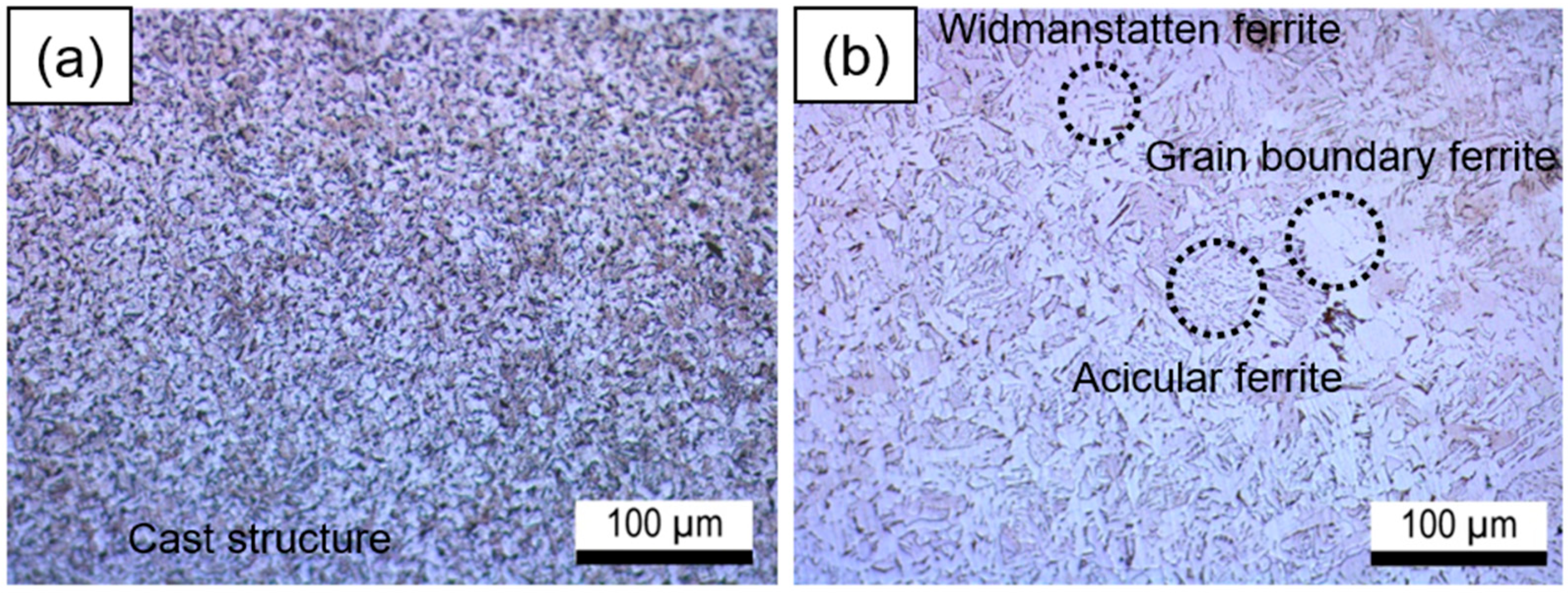
Figure 3 depicts the optical micrographs of the HAZ and the weld metal. The weld metal exhibited a fine grain size (Figure 3a). However, due to the heat generated during the welding process, the HAZ exhibited a larger grain size than the weld metal (Figure 3b) [21]. The weld metal had a cast structure, while the HAZ was composed of widmanstatten ferrite, grain boundary ferrite, and acicular ferrite. The electrochemical behavior of the HAZ is influenced by the complex microstructures, which may decrease the polarization resistance [7,22,23,24].

3.2. Potentiodynamic Test

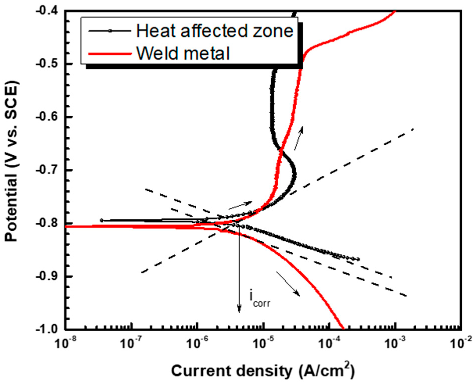
The potentiodynamic test was performed to examine the corrosion current density of the weldment of pipeline steel in DH water, and the results are shown in Figure 4. To compute the corrosion current density, the Tafel extrapolation method was used [25]. Equation (3) describes the linear relationship between the overpotential and the log scale current density:
η = a ± β(a,c)log|i|, a = −βalog(i0) or βclog(i0), βa ≅ (RT/(1 − α)nF), βc ≅ (RT/αnF)
where βa represents the anodic Tafel slope, βc represents the cathodic Tafel slope, i0 represents the exchange current density, α represents the charge transfer coefficient, n represents the charge number, R represents the gas constant (8.314 J/(mol∙K)), and T represents the absolute temperature (K). From Equation (3), a linear relationship was derived, and the corrosion current density of the HAZ was measured at 4.304 μA/cm2, and the corrosion current density of the weld metal was measured at 2.569 μA/cm2 according to the polarization curves as shown in Figure 4 and Table 3. As a result, the HAZ is more prone to corrosion than the weld metal [26,27].

3.3. Corrosion Acceleration Test

The testing conditions, including applied current density and test time, were determined based on the corrosion current density of the HAZ (4.304 μA/cm2) using Faraday’s law, and the results are summarized in Table 4. To accelerate the specimen’s corrosion, a current density of 4 mA/cm2 was applied. Figure 5 confirms that all specimens experienced uniform corrosion after the galvanostatic test. However, due to the more noble corrosion potential of the weld metal compared to the HAZ, a difference in the corrosion depth between the HAZ and weld metal was observed. Therefore, the corrosion depth of the HAZ was measured using a 3D profiler, and the results are presented in Table 5.

3.4. Regression Analysis and Validation of the Formula

Through multiple regression analysis using Minitab 19 software, the relationship between the experimental factors (pH, DO, and operating time) and corrosion depth was derived as follows.
Corrosion depth (μm) = −133 + 17.1 pH + 0.00072 DO + 125.2 Time − 7.95 pH × Time + 0.002921 DO × Time
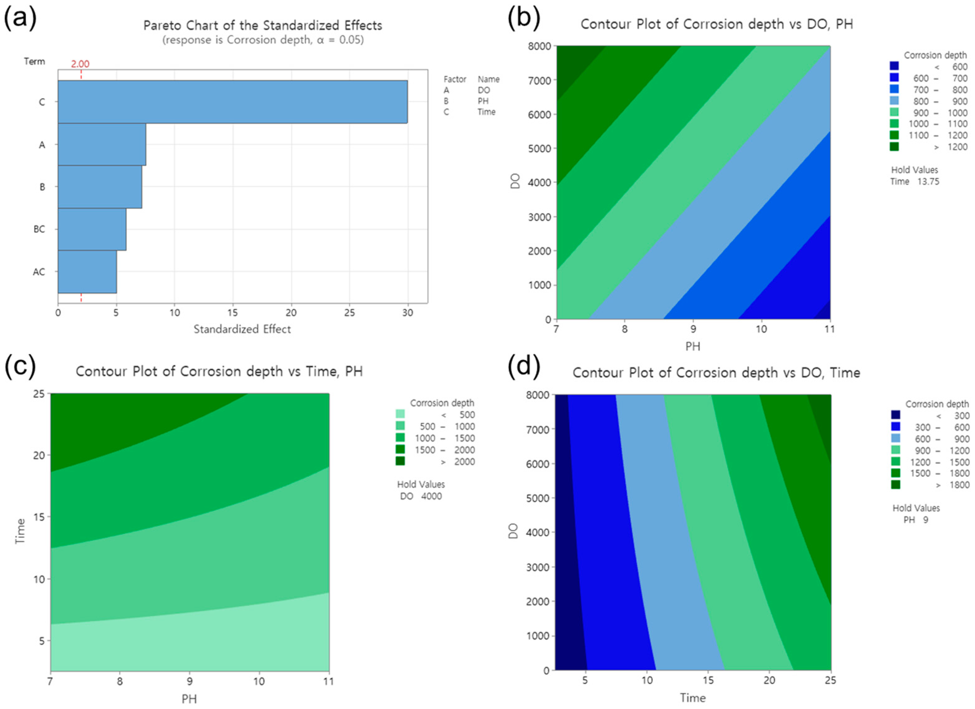
The effect of various factors on corrosion depth was analyzed using RSM, and the results are presented in Figure 6. As shown in Figure 6a, the standardized effect of the factors appeared in the order of operating time, DO, and pH. The significance of each factor was determined using the Pareto chart, where the T-value was used to measure the coefficient’s significance with respect to the standard error [28,29,30,31,32]. The operating time was found to have the greatest influence on the corrosion depth. The bars that represent all factors on the Pareto chart cross the reference line at 2.00, indicating that these factors are statistically significant at the 0.05 level based on the current model [33].
To better understand the effect of each factor on the corrosion depth, two-dimensional (2D) surface contour plots were generated. Three different factors were examined, but the 2D plots could only represent two factors and the corrosion depth (response). Therefore, one factor had to be fixed as a constant value. Figure 6b presents the 2D plot demonstrating the effects of the DO and pH on the corrosion depth. With a fixed value of 13.75 years for time, the effect of the DO increased with the increasing DO concentration, resulting in a corrosion depth from 900 μm to 1200 μm. Conversely, the effect of pH on corrosion decreased with increasing the pH, resulting in a corrosion depth from 1000 μm to 600 μm. In Figure 6c, holding the DO constant at 4000 ppb, the corrosion depth increased from 500 μm to 2000 μm with an increase in the operating time. In Figure 6d, with a fixed pH value of 9, the corrosion depth increased from 300 μm to 1800 μm with an increase in the operating time. Consequently, in the DH water, the effect of the operating time had a greater effect on the corrosion depth than the pH and DO, especially within the pH range from 7 to 11 and the DO range from 0 to 8000 ppb.
The suitability of the formula was assessed through the coefficient of determination (R2) and analysis of variance (ANOVA). The R2 value explains the percentage of variation in the response variable [34,35]. R2 can have a value between 0 and 1, and a value close to 1 indicates a good relationship between experimental and predicted values [36]. In this formula, the R2 value was 0.95. ANOVA was used to study whether certain parameters had a substantial impact. To conduct ANOVA, the sum of squares is usually converted into contributions from the regression model and the residual error. In Table 6, the model, p-value, F-value, and associated probability values are reported to verify the significance of the model. The decision value is the p-value, which is usually set to <0.05 [37,38,39,40] to indicate model validation, and the F-value shows the impact of the process parameter on the response [41]. Therefore, when the p-value output from the ANOVA of this research is 0.00 (<0.05), there is a substantial difference between the variables. Here, all parameters have a substantial impact on the corrosion depth when their p-value is <0.05. Additionally, a lack-of-fit test was performed using ANOVA [42]. The lack-of-fit means that the multiregression model obtained through the experiments is not suitable to explain the data. In a lack-of-fit test, the null hypothesis is that “the model is good at explaining the data”. Thus, the regression model can be assessed to be meaningful only when the null hypothesis is not rejected because the p-value computed through the lack-of-fit test is greater than the significance level. As a result of the analysis, the R2 value was 0.95, and ANOVA verified that the p-value for the model and each coefficient showed a high confidence level at the significance level of 0.05. Therefore, the analysis and observation reiterate a good correlation between the experimental findings and the values predicted using the statistical model, which demonstrates the success of this model.

3.5. Corrosion Depth Prediction

Using the derived formula, the corrosion depth of the HAZ can be predicted based on the levels of corrosion factors. Since DH pipelines are buried in soil, it can be difficult to directly manage their corrosion. Therefore, the corrosion factors in DH water were monitored to indirectly predict the corrosion depth of the HAZ. The pH and DO levels in the DH water were measured every 30 min over a period of 250 days under operating conditions, and the results are presented in Figure 7. The pH was observed to remain stable between 9 and 10, which is within the management standard for DH water. However, the DO concentration exceeded the management standards of 200 ppb several times. Based on these results, the average values of corrosion factors were applied to the formula, and Table 7 displays the predicted depth of corrosion in the DH pipeline HAZ over time. This method is expected to provide an indirect means of examining the corrosion depth of the DH pipeline steel weldment.

4. Conclusions

In this research, galvanostatic acceleration was utilized to simulate the long-term corrosion of the DH pipeline weldment based on the corrosion factors. Following the measurement of corrosion depth, a multiple regression analysis was conducted to establish the relationship between corrosion depth and corrosion factors, namely, pH, DO, and operating time. The results of the R2 and ANOVA of the derived formula showed a high level of suitability. Additionally, an example of how the formula can be applied was presented. This approach can be extended to evaluate the corrosion of structures that are difficult to manage directly by measuring corrosion factors in the operating environment.

Author Contributions

Conceptualization, Y.-S.S. and W.-C.K.; methodology, Y.-S.S. and J.-M.L.; validation, S.-J.K. and W.-C.K.; investigation, J.-M.L. and S.-J.K.; writing—original draft preparation, Y.-S.S.; writing—review and editing, J.-G.K.; supervision, J.-G.K. All authors have read and agreed to the published version of the manuscript.

Funding

This research was supported by the Korea District Heating Corporation (no. 0000000014524). This research was supported by Sungkyunkwan University and the BK21 FOUR (Graduate School Innovation) funded by the Ministry of Education (MOE, Korea) and National Research Foundation of Korea (NRF).

Institutional Review Board Statement

Not applicable.

Informed Consent Statement

Not applicable.

Data Availability Statement

Data is contained within the article material.

Conflicts of Interest

The authors declare no conflict of interest.

References

  1. Rezaie, B.; Rosen, M.A. District heating and cooling: Review of technology and potential enhancements. Appl. Energy 2012, 93, 2–10. [Google Scholar] [CrossRef]
  2. Werner, S. International review of district heating and cooling. Energy 2017, 137, 617–631. [Google Scholar] [CrossRef]
  3. Ezzeldin, I.; El Naggar, H.; Newhook, J.; Jarjoura, G. Accelerated wet/dry corrosion test for buried corrugated mild steel. Case Stud. Constr. Mater. 2022, 17, e01152. [Google Scholar] [CrossRef]
  4. Niazi, H.; Eadie, R.; Chen, W.; Zhang, H. High pH stress corrosion cracking initiation and crack evolution in buried steel pipelines: A review. Eng. Fail. Anal. 2020, 120, 105013. [Google Scholar] [CrossRef]
  5. Saheb, M.; Neff, D.; Dillmann, P.; Matthiesen, H.; Foy, E. Long-term corrosion behaviour of low-carbon steel in anoxic environ-ment: Characterisation of archaeological artefacts. J. Nucl. Mater. 2008, 379, 118–123. [Google Scholar] [CrossRef]
  6. Kim, S.; So, Y.; Kim, J. Fracture behavior of locally corroded steel pipeline in district heating system using the com-bination of electrochemistry and fracture mechanics. Met. Mater. Int. 2020, 26, 1671–1678. [Google Scholar] [CrossRef]
  7. Kim, Y.-S.; Kim, J.-G. Investigation of Weld Corrosion Effects on the Stress Behavior of a Welded Joint Pipe Using Numerical Simulations. Met. Mater. Int. 2019, 25, 918–929. [Google Scholar] [CrossRef]
  8. Kim, S.; Chun, K.; Kang, K.; Baik, M.; Kwon, S.; Choi, J. Estimation of the corrosion thickness of a disposal container for high-level radioactive wastes in a wet bentonite. J. Ind. Eng. Chem. 2007, 13, 959–964. [Google Scholar]
  9. Dahal, K.P.; Timilsena, J.N.; Gautam, M.; Bhattarai, J. Investigation on Probabilistic Model for Corrosion Failure Level of Buried Pipelines in Kirtipur Urban Areas (Nepal). J. Fail. Anal. Prev. 2021, 21, 914–926. [Google Scholar] [CrossRef]
  10. Hong, M.-S.; So, Y.-S.; Lim, J.-M.; Kim, J.-G. Evaluation of internal corrosion property in district heating pipeline using fracture mechanics and electrochemical acceleration kinetics. J. Ind. Eng. Chem. 2020, 94, 253–263. [Google Scholar] [CrossRef]
  11. Chung, N.T.; Choi, S.-R.; Kim, J.-G. Comparison of Response Surface Methodologies and Artificial Neural Network Approaches to Predict the Corrosion Rate of Carbon Steel in Soil. J. Electrochem. Soc. 2022, 169, 051503. [Google Scholar] [CrossRef]
  12. Aghaaminiha, M.; Mehrani, R.; Colahan, M.; Brown, B.; Singer, M.; Nesic, S.; Vargas, S.; Sharma, S. A novel green corrosion inhibitor extracted from waste feverfew root for carbon steel in H2SO4 solution. Corros. Sci. 2021, 193, 100971. [Google Scholar]
  13. Myers, R.; Montgomery, D.; Anderson-Cook, C. Response Surface Methodology: Process and Product Optimization Using Designed Experiments; John Wiley & Sons: New York, NY, USA, 2016; pp. 3–21. [Google Scholar]
  14. Rajkumar, K.; Muthukumar, M. Response surface optimization of electro-oxidation process for the treatment of C.I. Reactive Yellow 186 dye: Reaction pathways. Appl. Water Sci. 2015, 7, 637–652. [Google Scholar] [CrossRef]
  15. Rashid, K.H.; Khadom, A.A. Optimization of inhibitive action of sodium molybdate (VI) for corrosion of carbon steel in saline water using response surface methodology. Korean J. Chem. Eng. 2019, 36, 1350–1359. [Google Scholar] [CrossRef]
  16. So, Y.; Hong, M.; Lim, J.; Kim, W.; Kim, J. Calibrating the impressed anodic current density for accelerated gal-vanostatic testing to simulate the long-term corrosion behavior of buried pipeline. Materials 2021, 14, 2100. [Google Scholar] [CrossRef]
  17. Sharma, Y.; Srivastava, V.; Singh, V.; Kaul, S.; Weng, C.-H. Nano-adsorbents for the removal of metallic pollutants from water and wastewater. Environ. Technol. 2009, 30, 583–609. [Google Scholar] [CrossRef]
  18. Goh, K.-H.; Lim, T.-T.; Chui, P.-C. Evaluation of the effect of dosage, pH and contact time on high-dose phosphate inhibition for copper corrosion control using response surface methodology (RSM). Corros. Sci. 2008, 50, 918–927. [Google Scholar] [CrossRef]
  19. Chung, N.T.; So, Y.-S.; Kim, W.-C.; Kim, J.-G. Evaluation of the Influence of the Combination of pH, Chloride, and Sulfate on the Corrosion Behavior of Pipeline Steel in Soil Using Response Surface Methodology. Materials 2021, 14, 6596. [Google Scholar] [CrossRef]
  20. Montgomery, D.P.; A Plate, C.; Jones, M.; Jones, J.; Rios, R.; Lambert, D.K.; Schumtz, N.; E Wiedmeier, S.; Burnett, J.; Ail, S.; et al. Using umbilical cord tissue to detect fetal exposure to illicit drugs: A multicentered study in Utah and New Jersey. J. Perinatol. 2008, 28, 750–753. [Google Scholar] [CrossRef]
  21. Kou, S. Welding Metallurgy, 2nd ed.; John Wiley & Sons Inc.: Hoboken, NJ, USA, 2003; pp. 393–412. [Google Scholar]
  22. Zhu, J.; Xu, L.; Feng, Z.; Frankel, G.; Lu, M.; Chang, W. Galvanic corrosion of a welded joint in 3Cr low alloy pipeline steel. Corros. Sci. 2016, 111, 391–403. [Google Scholar] [CrossRef]
  23. Cao, X.; Wu, T.; Liu, M.; Wang, B.; Zhang, M.; Li, C.; Yin, F. Corrosion behavior of the weld joint of X80 pipeline steel in an acidic red soil. Mater. Res. Express 2020, 7, 036527. [Google Scholar] [CrossRef]
  24. Huang, H.-H.; Tsai, W.-T.; Lee, J.-T. The influences of microstructure and composition on the electrochemical behavior of a516 steel weldment. Corros. Sci. 1994, 36, 1027–1038. [Google Scholar] [CrossRef]
  25. Jones, D.A. Principles and Prevention of Corrosion, 2nd ed.; Prentice Hall: Hoboken, NJ, USA, 1992; pp. 75–83. [Google Scholar]
  26. Richter, S.; Thorarinsdottir, R.; Jonsdottir, F. On-line corrosion monitoring in geothermal district heating systems. II. Localized corrosion. Corros. Sci. 2007, 49, 1907–1917. [Google Scholar] [CrossRef]
  27. Hilbert, L. Monitoring corrosion rates and localised corrosion in low conductivity water. Corros. Sci. 2006, 48, 3907–3923. [Google Scholar] [CrossRef]
  28. Lourenço, J.C.; Faria, M.I.S.T.; Robin, A.; Prisco, L.P.; Puccini, M. Influence of process parameters on localized corrosion of AA7075 alloy during the production of aeronautic components. Mater. Corros. 2015, 66, 1498–1503. [Google Scholar] [CrossRef]
  29. Parker, M.E.; Kelly, R.G.; Yan, Y.; Peguet, L.; Gharbi, O.; Deschamps, A.; Hutchinson, C.; Kairy, S.; Birbilis, N.; Karayan, A.I.; et al. Investigating the Impact of Accelerated Testing Variables on the Exfoliation Corrosion of AA2060. Corrosion 2016, 72, 1342–1350. [Google Scholar] [CrossRef]
  30. Blanco, G.; Bautista, M.A.; Takenouti, H. EIS study of passivation of austenitic and duplex stainless steels reinforcements in simulated pore solutions. Cem. Concr. Compos. 2006, 28, 212–219. [Google Scholar] [CrossRef]
  31. Cabrera, J.; Claisse, P.; Hunt, D. A statistical analysis of the factors which contribute to the corrosion of steel in Portland cement and silica fume concrete. Constr. Build. Mater. 1995, 9, 105–113. [Google Scholar] [CrossRef]
  32. Zhao, Y.; Zhang, X.; Jin, W. Influence of environment on the development of corrosion product-filled paste and a corrosion layer at the steel/concrete interface. Corros. Sci. 2017, 124, 1–9. [Google Scholar] [CrossRef]
  33. Jayasuriya, A.; Adams, M.P.; Bandelt, M.J. Understanding variability in recycled aggregate concrete mechanical properties through numerical simulation and statistical evaluation. Constr. Build. Mater. 2018, 178, 301–312. [Google Scholar] [CrossRef]
  34. Ahmadi, M.; Rahmani, K.; Rahmani, A.; Rahmani, H. Removal of benzotriazole by Photo-Fenton like process using nano zero-valent iron: Response surface methodology with a Box-Behnken design. Pol. J. Chem. Technol. 2017, 19, 104–112. [Google Scholar] [CrossRef]
  35. De Rosa, R.; Earl, D.; Bierwagen, G. Statistical evaluation of EIS and ENM data collected for monitoring corrosion barrier properties of organic coatings on Al-2024-T3. Corros. Sci. 2002, 44, 1607–1620. [Google Scholar] [CrossRef]
  36. Kazemi, M.; Ahangarani, S.; Esmailian, M.; Shanaghi, A. Investigating the corrosion performance of Ti-6Al-4V biomaterial alloy with hydroxyapatite coating by artificial neural network. Mater. Sci. Eng. B 2022, 278, 115644. [Google Scholar] [CrossRef]
  37. Martínez-Moreno, F.; Giraldo, P.; Nieto, C.; Ruiz, M. Resistance to Leaf and Yellow Rust in a Collection of Spanish Bread Wheat Landraces and Association with Ecogeographical Variables. Agronomy 2022, 12, 187. [Google Scholar] [CrossRef]
  38. Hernandez, S.; Nešić, S.; Weckman, G.; Ghai, V. Use of Artificial Neural Networks for Predicting Crude Oil Effect on Carbon Dioxide Corrosion of Carbon Steels. Corrosion 2006, 62, 467–482. [Google Scholar] [CrossRef]
  39. Hoang, N.-D. Image Processing-Based Pitting Corrosion Detection Using Metaheuristic Optimized Multilevel Image Thresholding and Machine-Learning Approaches. Math. Probl. Eng. 2020, 2020, 1–19. [Google Scholar] [CrossRef]
  40. Duarte, M.; Kostka, A.; Jimenez, J.; Choi, P.; Klemm, J.; Crespo, D.; Raabe, D.; Renner, F. Crystallization, phase evolution and corrosion of Fe-based metallic glasses: An atomic-scale structural and chemical characterization study. Acta Mater. 2014, 71, 20–30. [Google Scholar] [CrossRef]
  41. Di Leo, G.; Sardanelli, F. Statistical significance: p value, 0.05 threshold, and applications to radiomics—Reasons for a con-servative approach. Eur. Radiol. Exp. 2020, 4, 1–8. [Google Scholar] [CrossRef]
  42. Thirumalaikumarasamy, D.; Shanmugam, K.; Balasubramanian, V. Comparison of the corrosion behaviour of AZ31B magnesium alloy under immersion test and potentiodynamic polarization test in NaCl solution. J. Magnes. Alloy. 2014, 2, 36–49. [Google Scholar] [CrossRef]
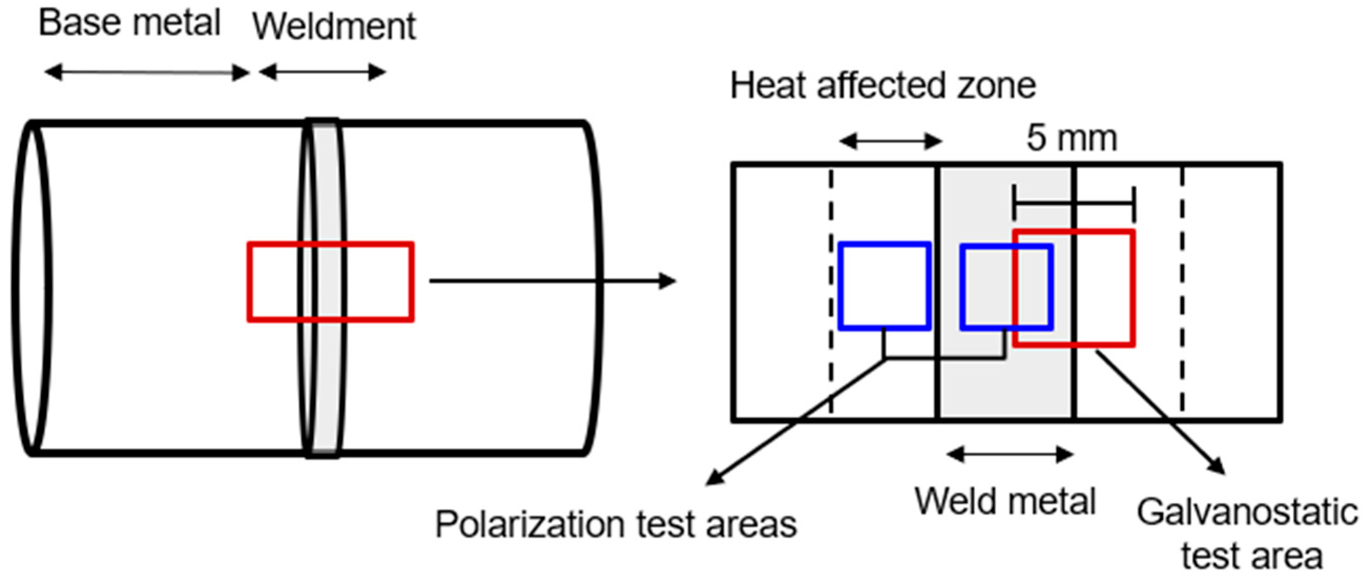
Figure 1. Schematic illustration of the sectioning procedures used to prepare the specimen from the DH pipeline weldment.
Materials 16 03254 g001
Figure 2. Corrosion depth examination process using a 3D profiler. (a) The corroded weldment after the galvanostatic test, (b) magnified image of the red square in (a), and (c) corrosion depth measurement.
Materials 16 03254 g002
Figure 3. Optical micrographs of the weldment: (a) weld metal; (b) heat-affected zone.
Materials 16 03254 g003
Figure 4. Polarization curves of the heat-affected zone and the weld metal of pipeline steel in the synthetic DH water.
Materials 16 03254 g004
Figure 5. Photographs of weldment after the corrosion acceleration. DO: (a) 0, (b) 200, (c) 1000, and (d) 8000 ppb.
Materials 16 03254 g005
Figure 6. Effect of factors in response surface analysis. (a) Pareto chart of the standardized effects, contour plots of corrosion depth vs. (b) DO and pH, (c) operating time and pH, (d) DO and operating time.
Materials 16 03254 g006
Figure 7. Actual monitoring data of pH and DO contained in DH water for 250 days.
Materials 16 03254 g007
Table 1. Composition of the DH pipeline materials (SPW400).
Composition (wt.%)
CMnPSFe
≤0.251.00≤0.04≤0.04Balance
Table 2. Composition of DH water.
pHTemp.NaCl
(mg/L)
Mg(OH)2
(mg/L)
CaCO3
(mg/L)
NH4OH
(mg/L)
10.060 °C15.010.482.6510.28
Table 3. Experimental conditions and calculated variables.
βa (V/dec.)βc (V/dec.)Ecorr (VSCE)icorr (A/cm2)
Heat-affected zone0.0840.039−0.7944.304 × 10−6
Weld metal0.0820.041−0.8072.569 × 10−6
Table 4. Computed testing conditions for the corrosion acceleration test.
In ServiceLaboratory
Impressed Anodic
Current Density
4.0 mA/cm2
Operating time21,900 h
(2.5 years)
Accelerated
test time
23.5 h
109,500 h
(12.5 years)
117.7 h
219,000 h
(25 years)
235.4 h
Table 5. The corrosion depth of the HAZ measured using a 3D profiler.
DO
(ppb)
Operating Time (Years)pHCorrosion
Depth (μm)
DO
(ppb)
Operating
Time (Years)
pHCorrosion
Depth (μm)
02.57126 ± 92002.57149 ± 10
8101 ± 128126 ± 13
9121 ± 159106 ± 14
10109 ± 1410108 ± 16
11169 ± 1811102 ± 13
12.57879 ± 3212.57936 ± 41
8598 ± 418728 ± 35
9606 ± 459732 ± 27
10694 ± 3610741 ± 34
11671 ± 2811671 ± 21
2571644 ± 862571860 ± 101
81079 ± 5781279 ± 77
91144 ± 6291248 ± 68
101074 ± 52101200 ± 70
111087 ± 43111235 ± 60
10002.57171 ± 1480002.57265 ± 15
8199 ± 218204 ± 21
9146 ± 179216 ± 13
10188 ± 2610230 ± 26
11121 ± 1311190 ± 9
12.571040 ± 6812.571240 ± 47
8845 ± 4681019 ± 62
9767 ± 499958 ± 42
10728 ± 3810962 ± 40
11679 ± 3211688 ± 21
2572248 ± 1222572604 ± 138
81643 ± 8882039 ± 121
91391 ± 9591892 ± 96
101215 ± 68101730 ± 102
111289 ± 69111422 ± 88
Table 6. Analysis of variance findings for the derived corrosion depth formula.
Degree of
Freedom
Sum of SquareMean SquareF-Valuep-Value
Model522,691,8274,538,365239.520.00
Linear321,527,0657,175,688378.720.00
pH11,185,2301,185,23062.550.00
DO11,087,5271,087,52757.400.00
Time119,056,25319,056,2531005.740.00
Interaction21,122,202561,10129.610.00
pH × Time1804,149804,14942.440.00
DO × Time1449,929449,92923.750.00
Error571,080,00318,947--
Lack of fit541,066,59119,7524.420.122
Pure error313,4124471--
Total6223,771,830---
Table 7. Monitoring data and predicted corrosion depth.
Averaged
pH
Averaged
DO (ppb)
Operating Time
(Year)
Predicted
Corrosion Depth
(μm)
Site A9.7654.372.5153.4
12.5631.0
25.01228.1
Disclaimer/Publisher’s Note: The statements, opinions and data contained in all publications are solely those of the individual author(s) and contributor(s) and not of MDPI and/or the editor(s). MDPI and/or the editor(s) disclaim responsibility for any injury to people or property resulting from any ideas, methods, instructions or products referred to in the content.