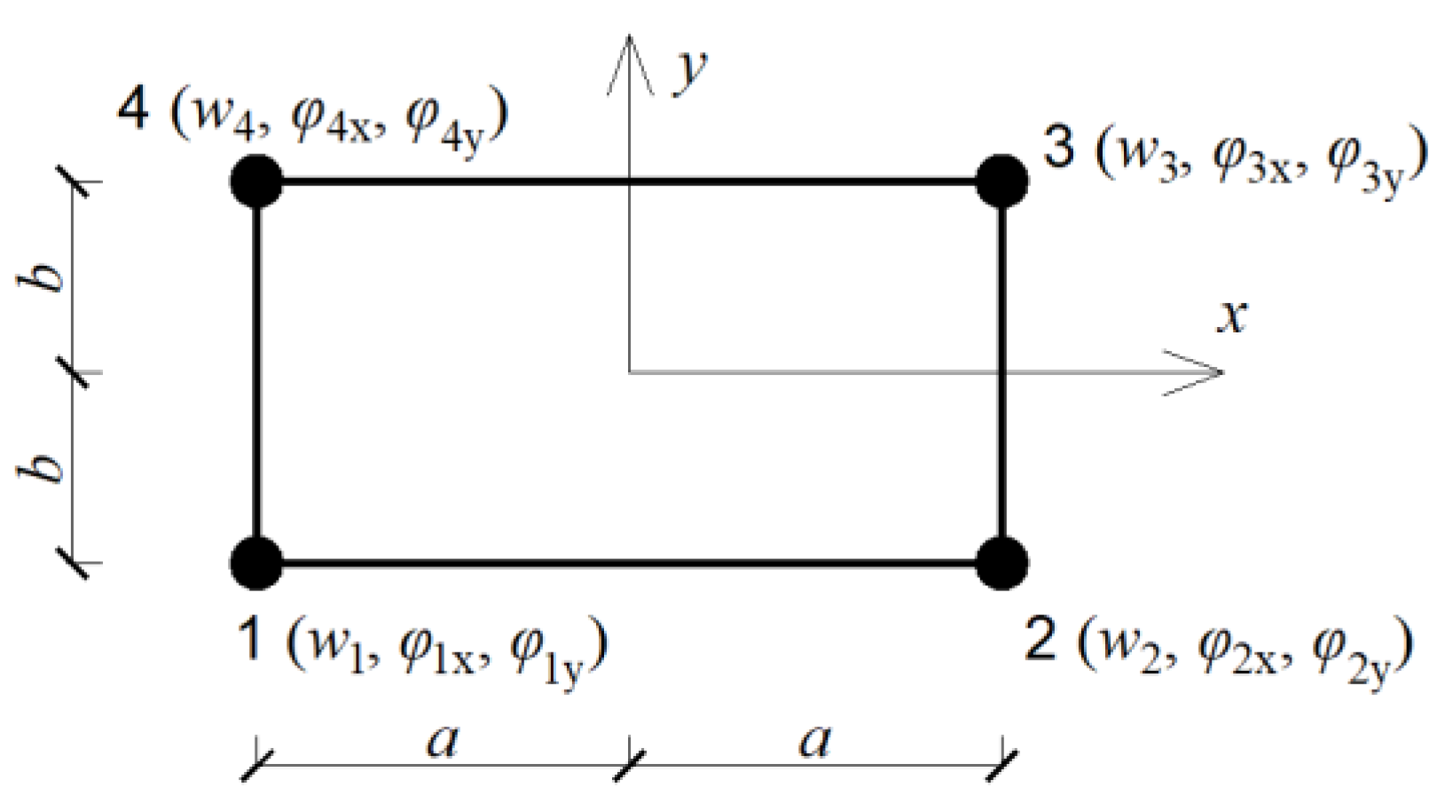
Figure 1.
Finite element used for discretization of tested plate: node numbering and active degrees of freedom.
Figure 1.
Finite element used for discretization of tested plate: node numbering and active degrees of freedom.
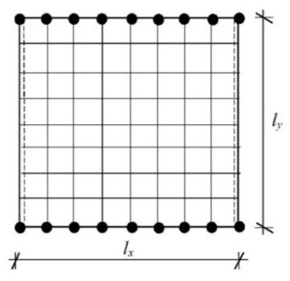
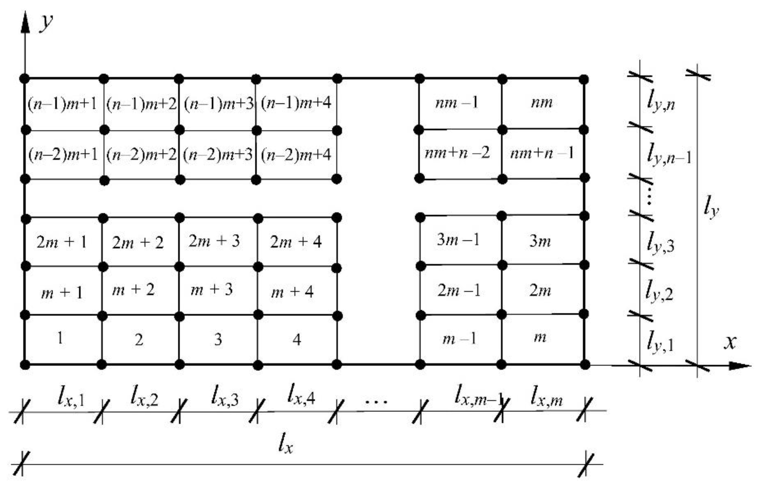
Figure 2.
Plate discretization with rectangular plate finite elements.
Figure 2.
Plate discretization with rectangular plate finite elements.
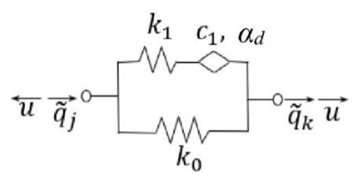
Figure 3.
The model of viscoelastic damper.
Figure 3.
The model of viscoelastic damper.
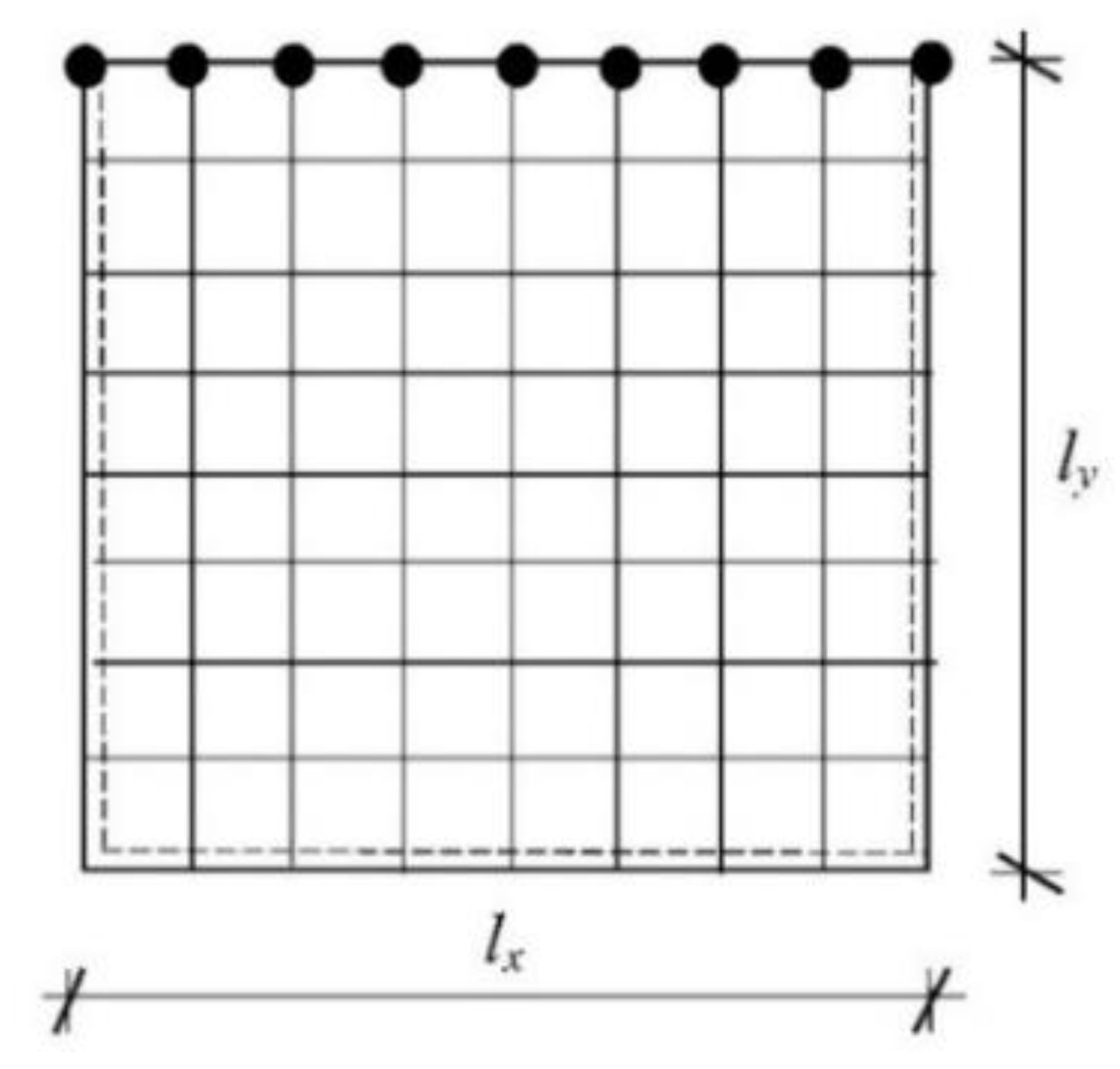
Figure 4.
Finite element mesh of the square isotropic plate simply supported on three adjacent edges, with the fourth edge resting on viscoelastic constraints.
Figure 4.
Finite element mesh of the square isotropic plate simply supported on three adjacent edges, with the fourth edge resting on viscoelastic constraints.
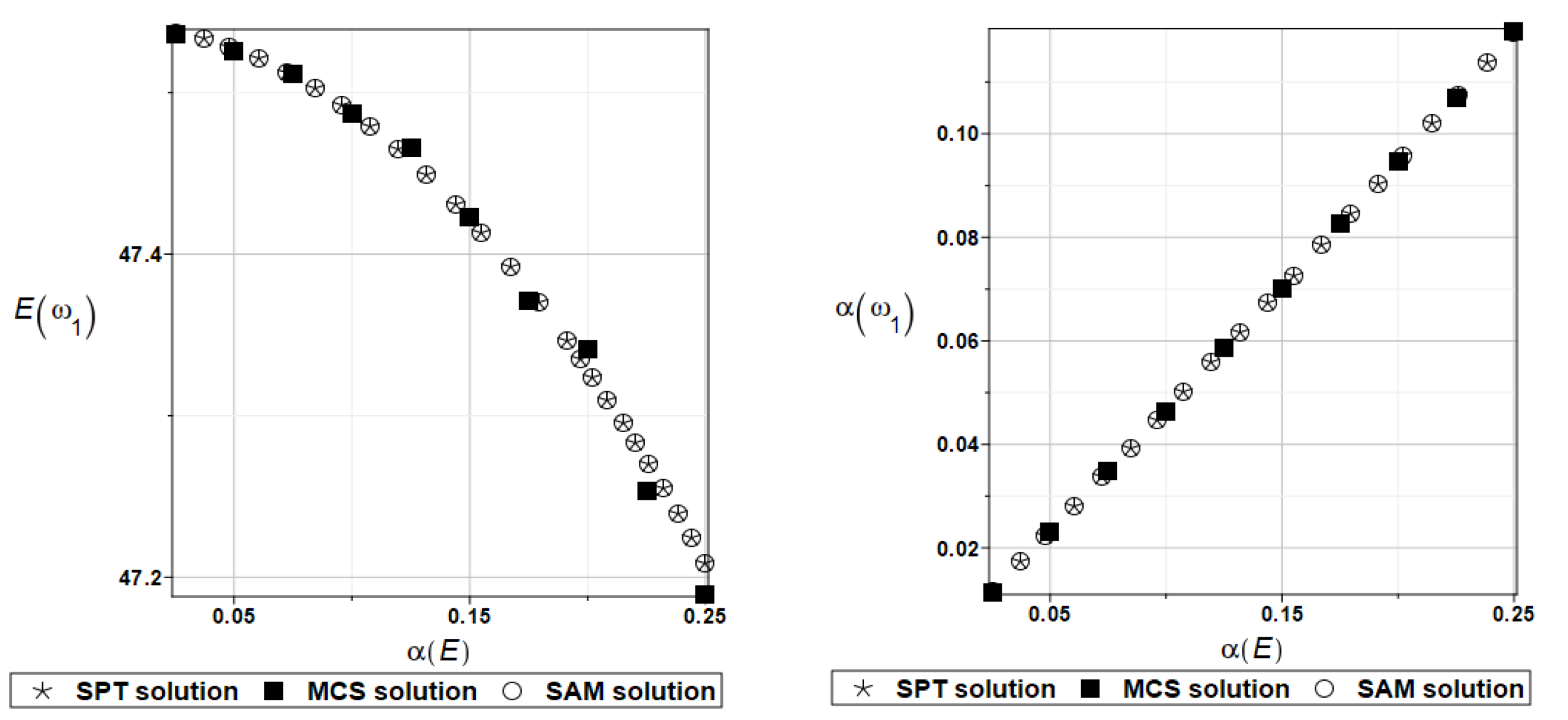
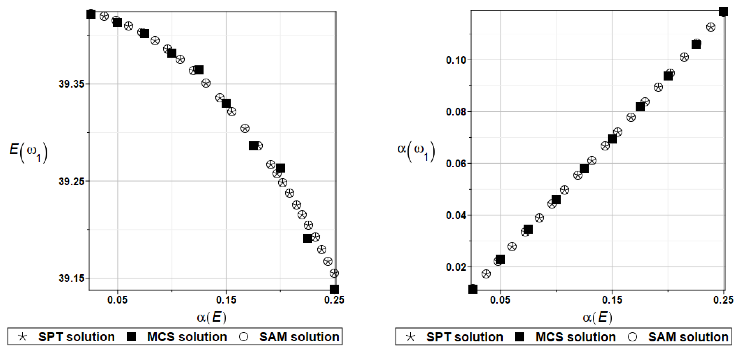
Figure 5.
Probabilistic moments for the first natural frequency and the random distribution of Young’s modulus.
Figure 5.
Probabilistic moments for the first natural frequency and the random distribution of Young’s modulus.
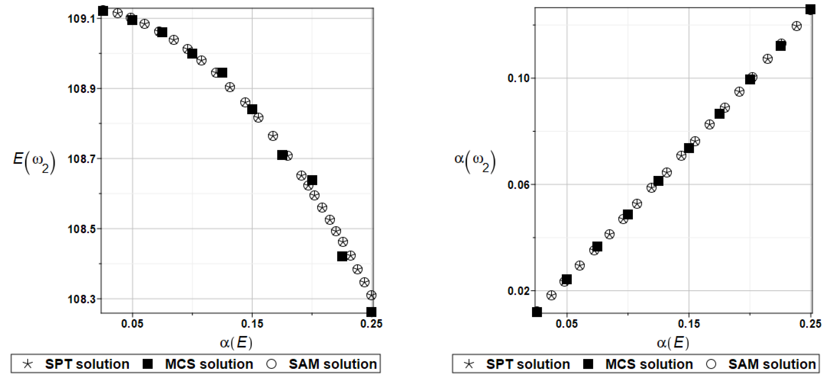
Figure 6.
Probabilistic moments for the second natural frequency and the random distribution of Young’s modulus.
Figure 6.
Probabilistic moments for the second natural frequency and the random distribution of Young’s modulus.
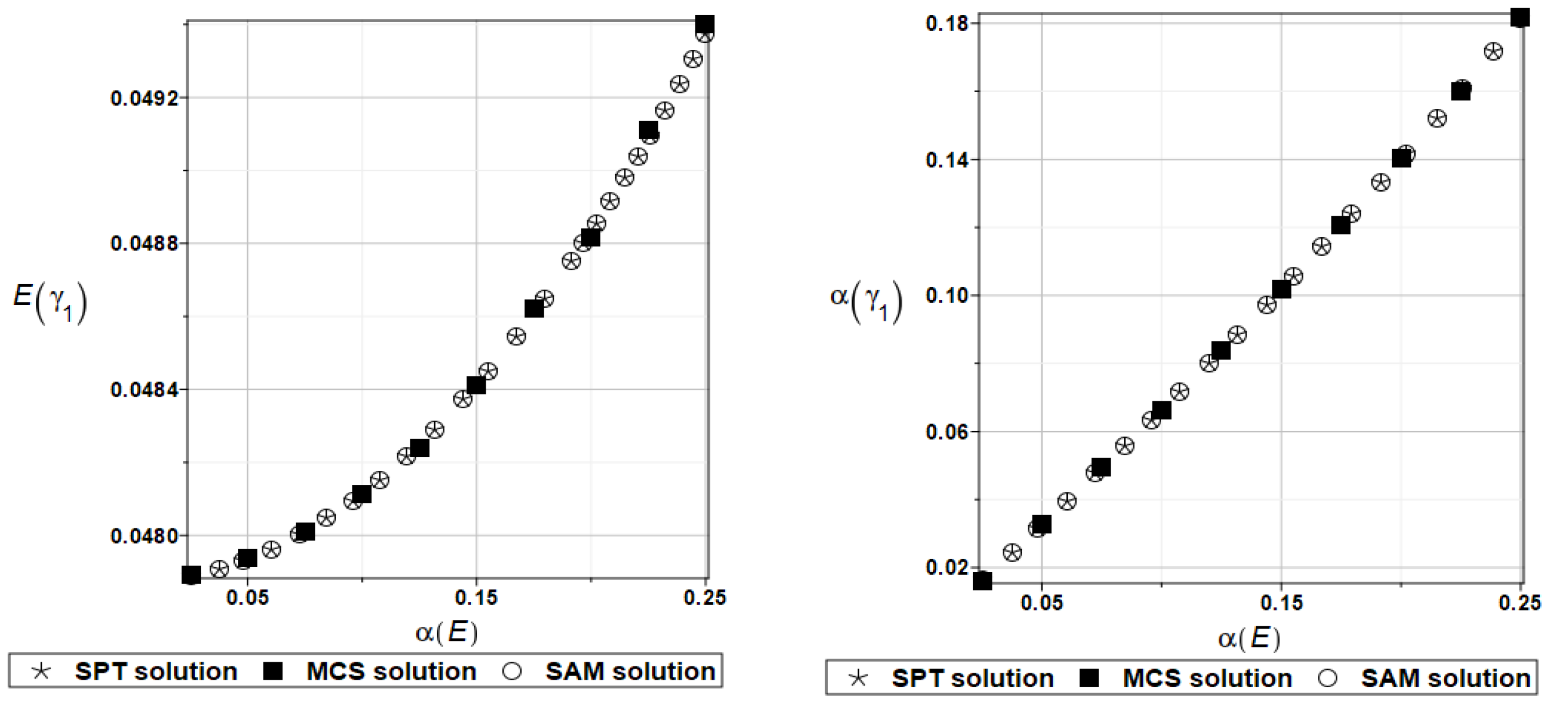
Figure 7.
Probabilistic moments for the first coefficient of damping and the random distribution of Young’s modulus.
Figure 7.
Probabilistic moments for the first coefficient of damping and the random distribution of Young’s modulus.
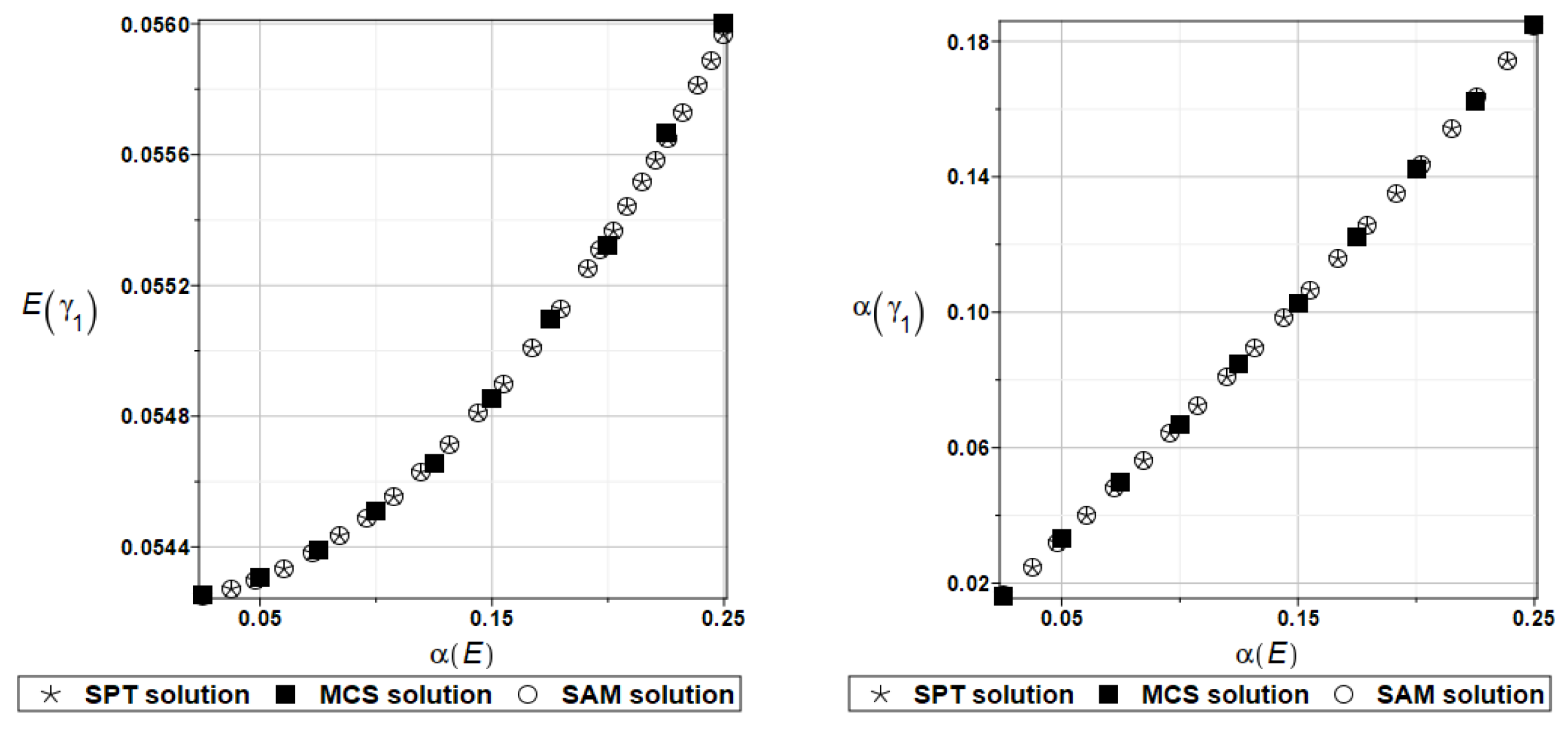
Figure 8.
Probabilistic moments for the second coefficient of damping and the random distribution of Young’s modulus.
Figure 8.
Probabilistic moments for the second coefficient of damping and the random distribution of Young’s modulus.
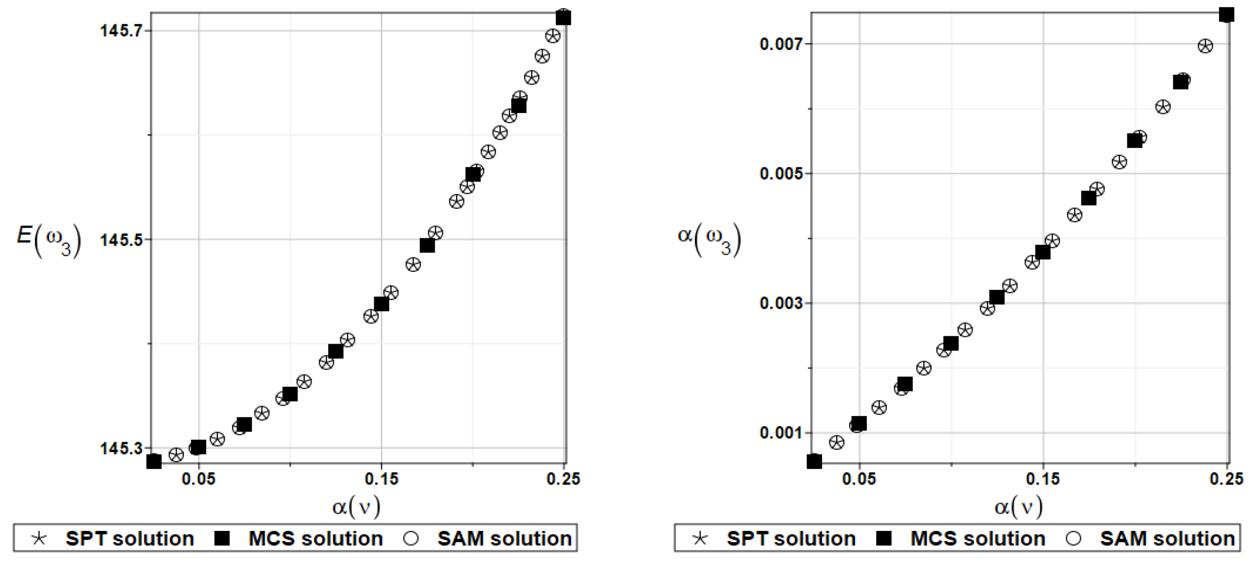
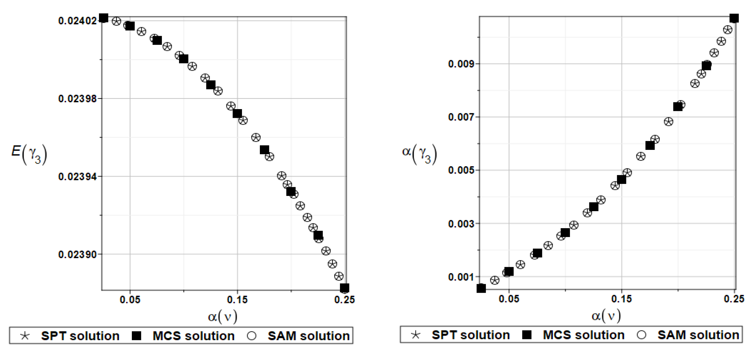
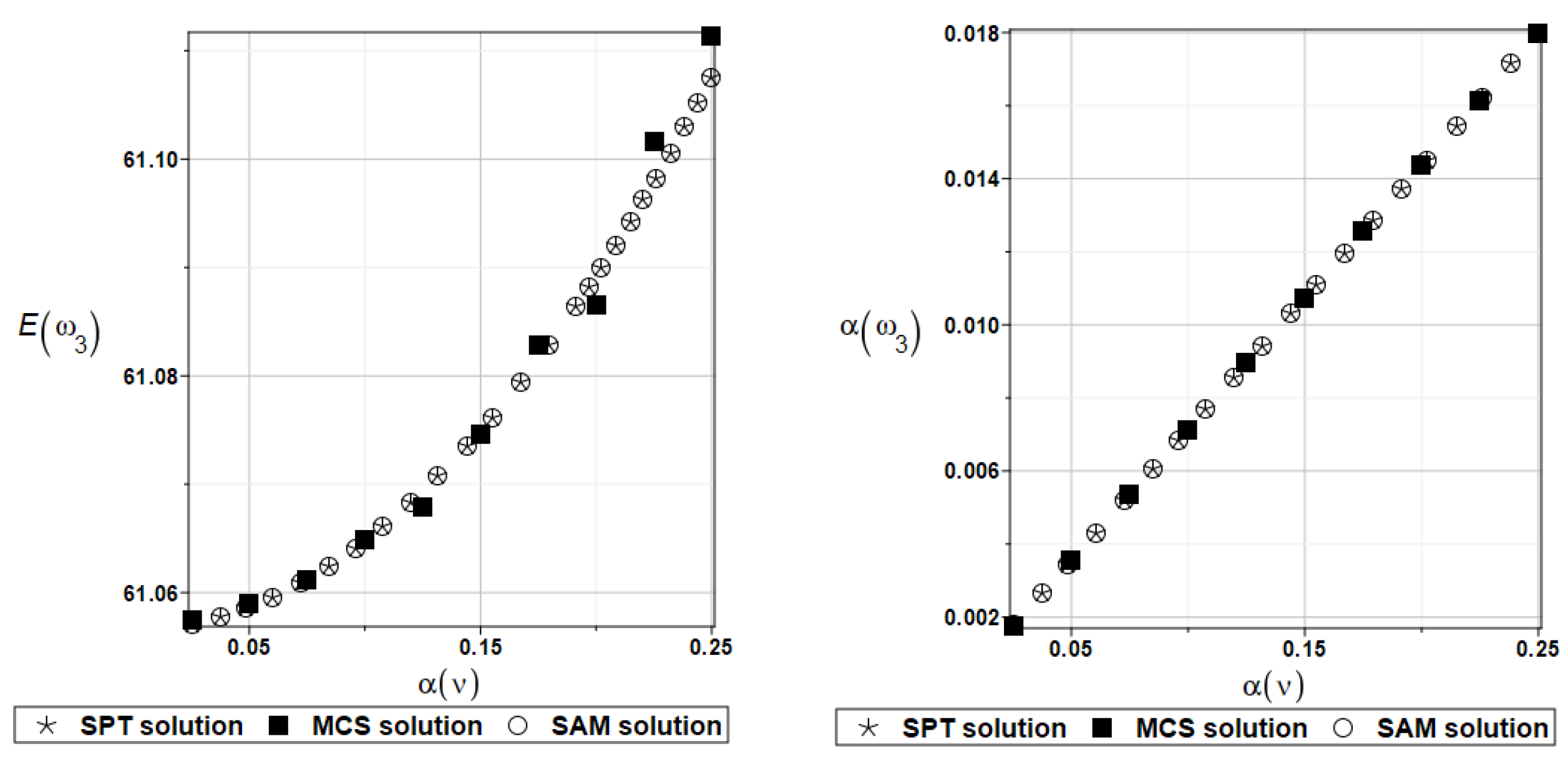
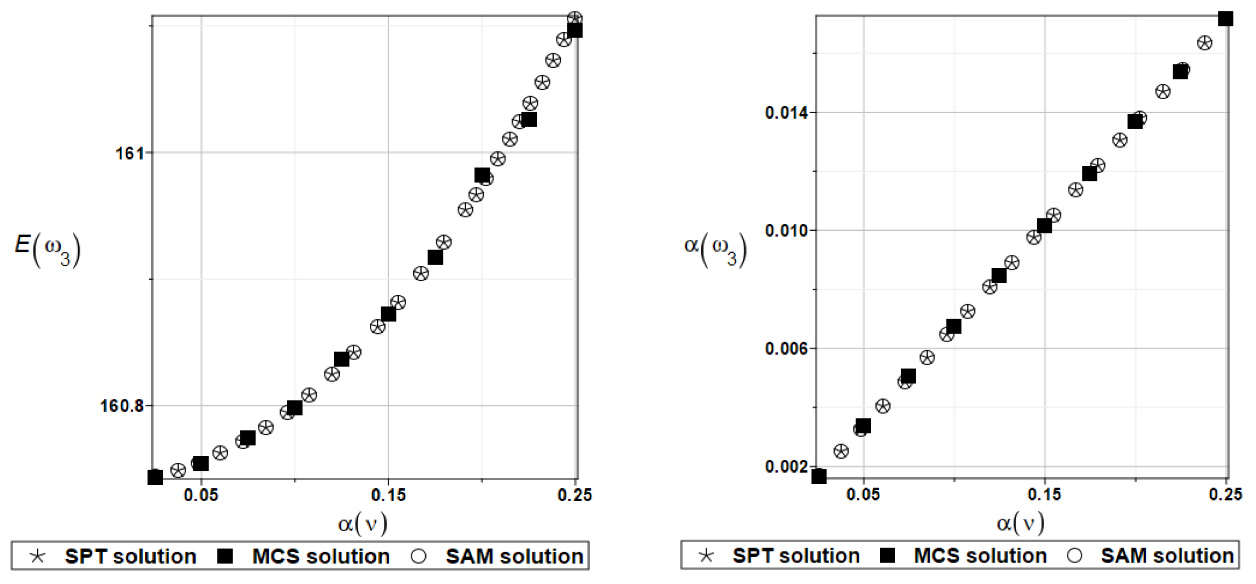
Figure 9.
Probabilistic moments for the third natural frequency and the random distribution of Poisson’s ratio.
Figure 9.
Probabilistic moments for the third natural frequency and the random distribution of Poisson’s ratio.
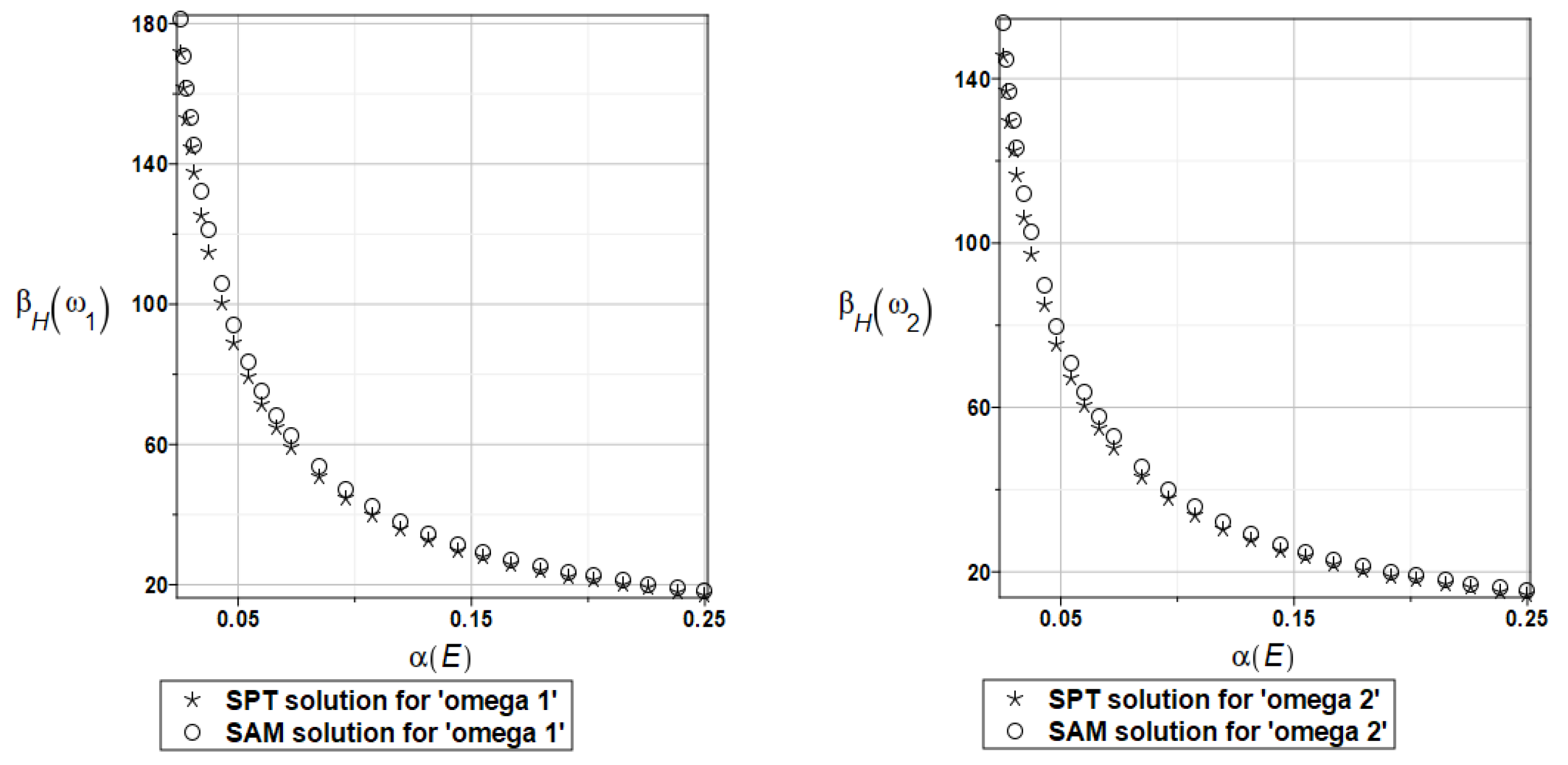
Figure 10.
Probabilistic moments for the first coefficient of damping and the random distribution of Poisson’s ratio.
Figure 10.
Probabilistic moments for the first coefficient of damping and the random distribution of Poisson’s ratio.
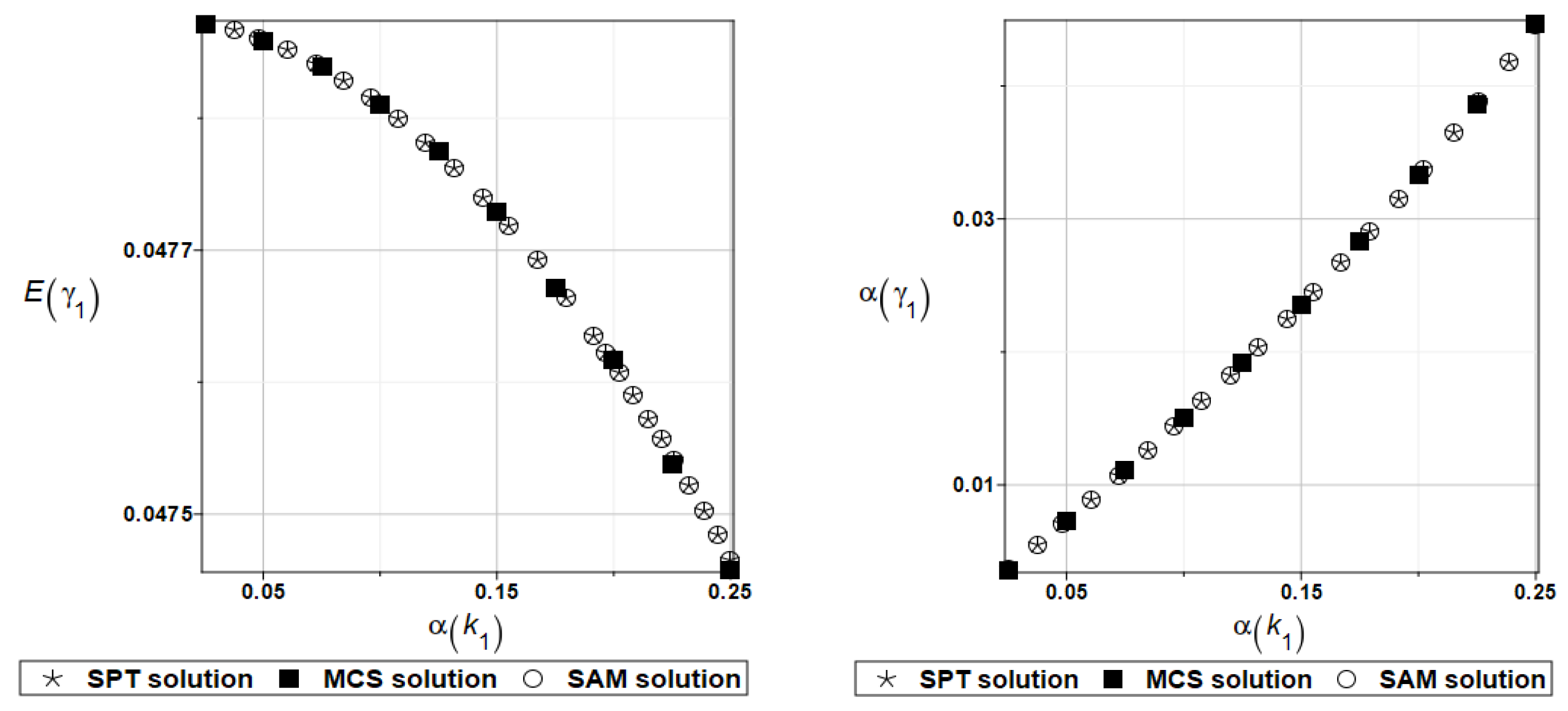
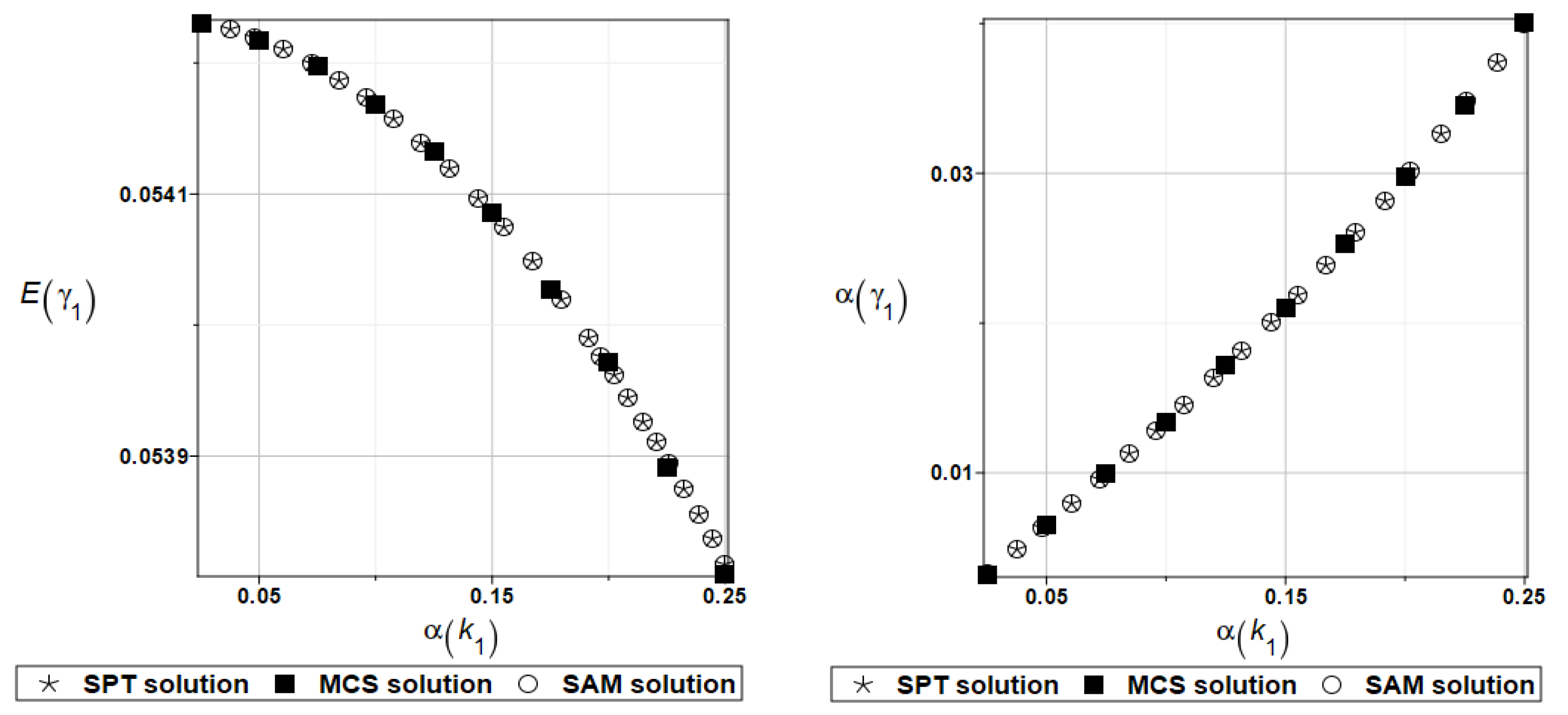
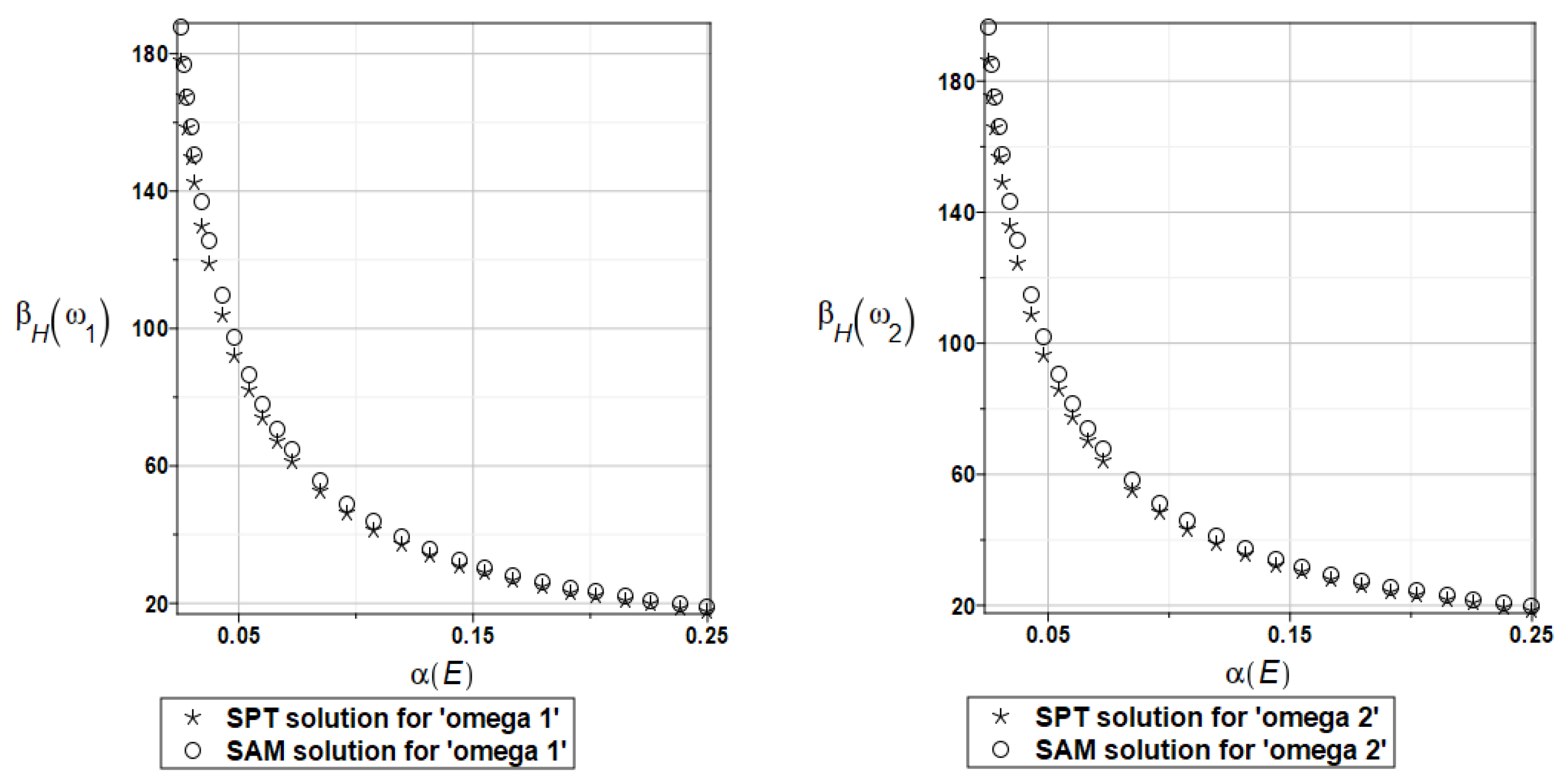
Figure 11.
Probabilistic moments for the first coefficient of damping and the random distribution of the damper’s parameter k1.
Figure 11.
Probabilistic moments for the first coefficient of damping and the random distribution of the damper’s parameter k1.
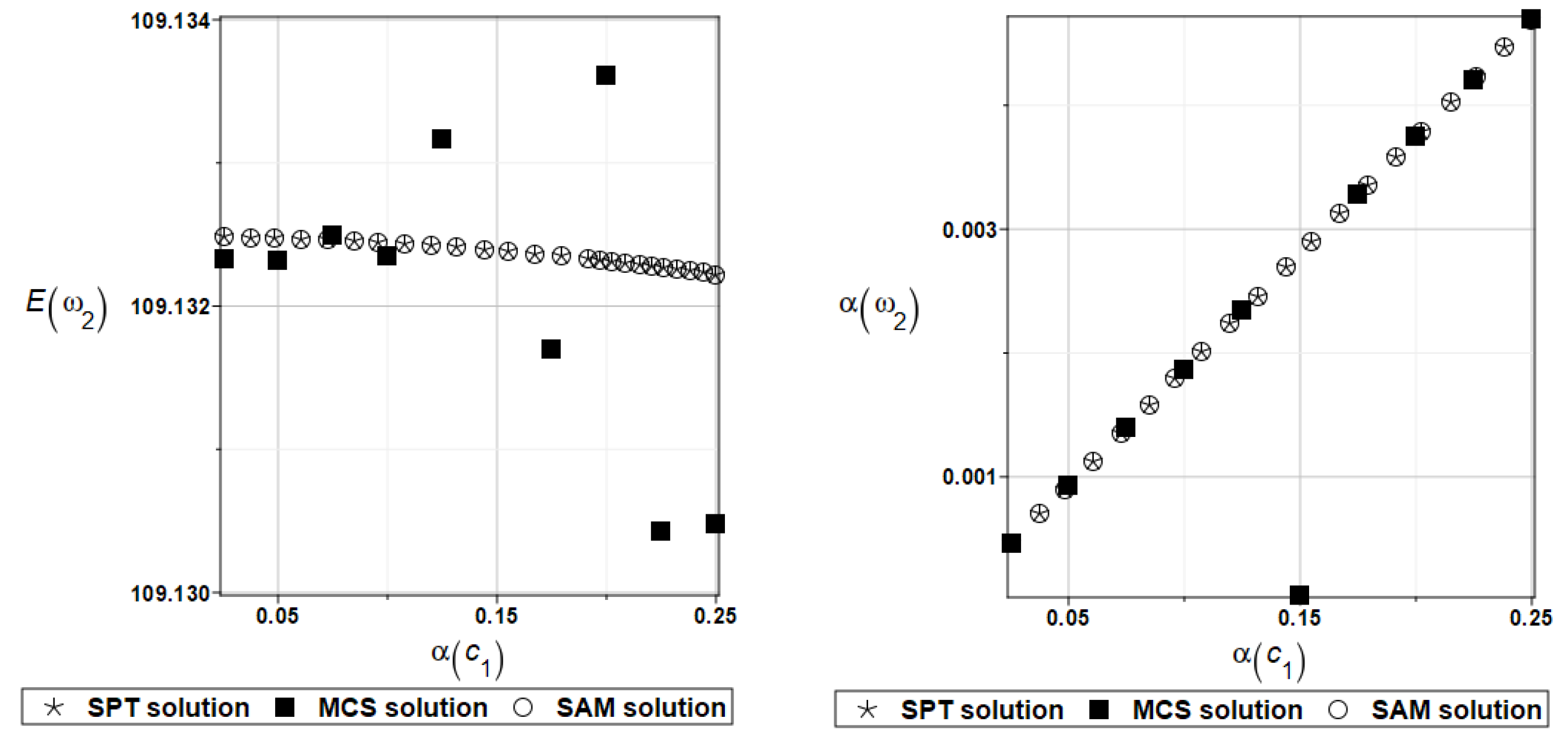
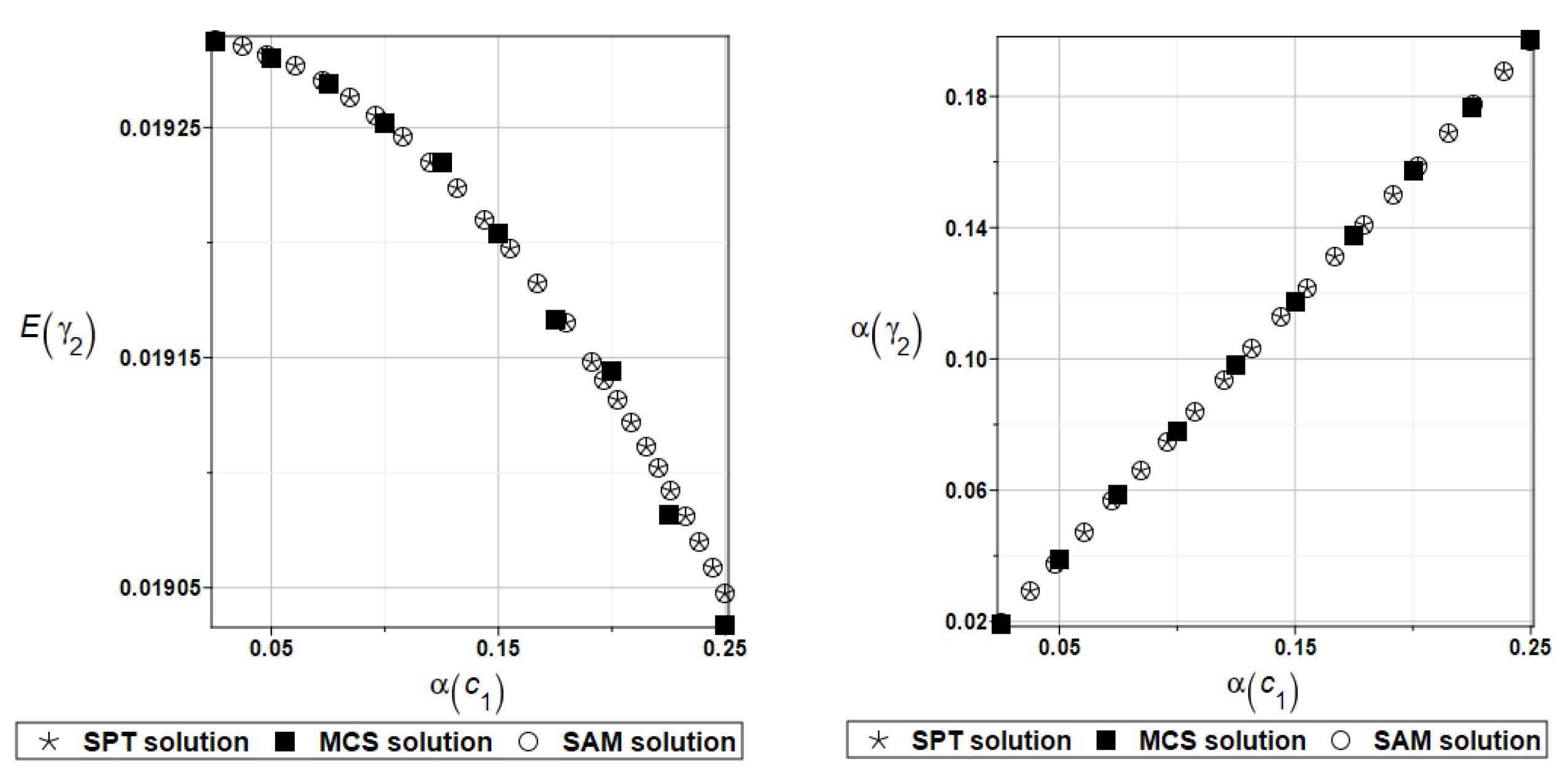
Figure 12.
Probabilistic moments for the second natural frequency and the random distribution of the damper’s parameter c1.
Figure 12.
Probabilistic moments for the second natural frequency and the random distribution of the damper’s parameter c1.
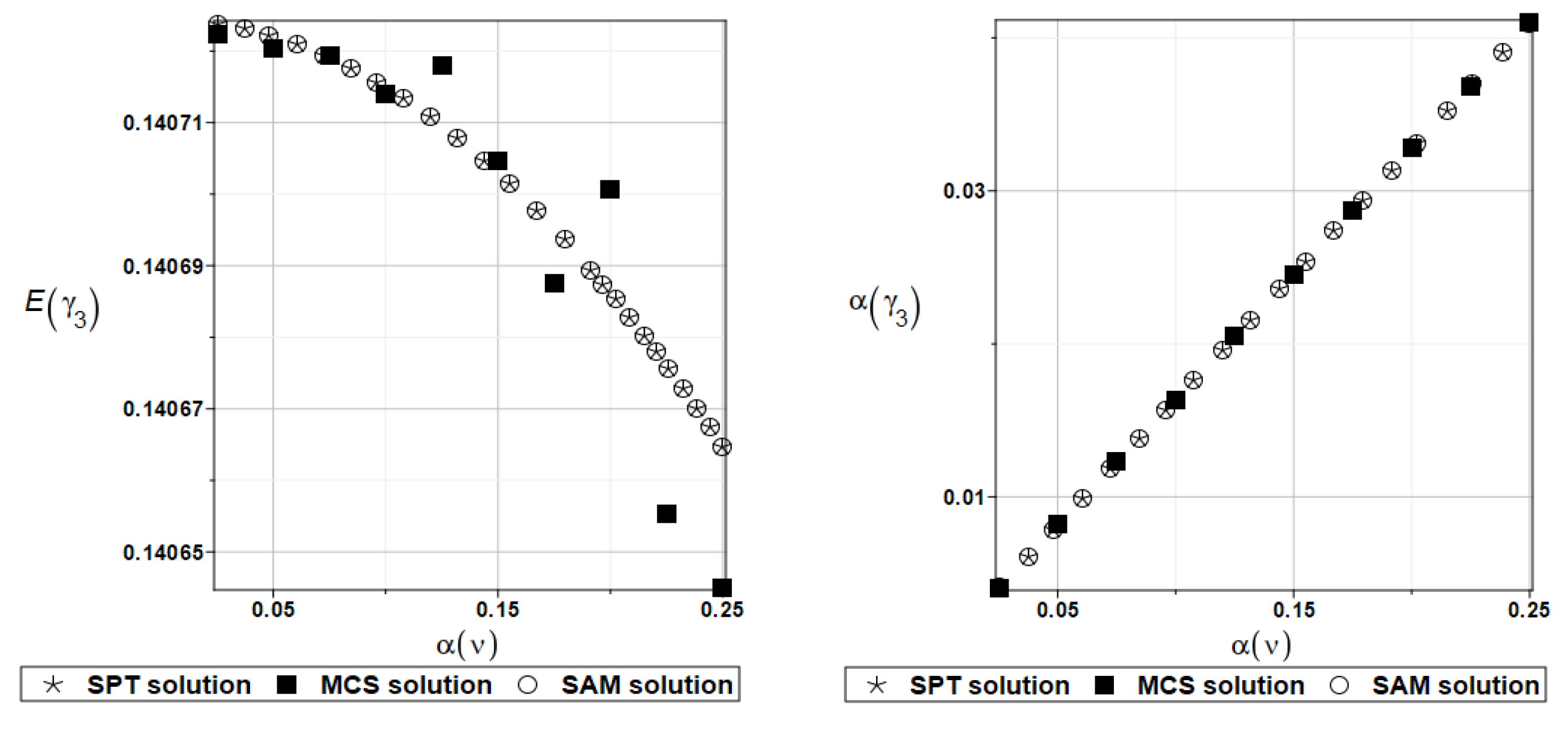
Figure 13.
Probabilistic moments for the coefficient of damping and the random distribution of the damper’s parameter c1.
Figure 13.
Probabilistic moments for the coefficient of damping and the random distribution of the damper’s parameter c1.
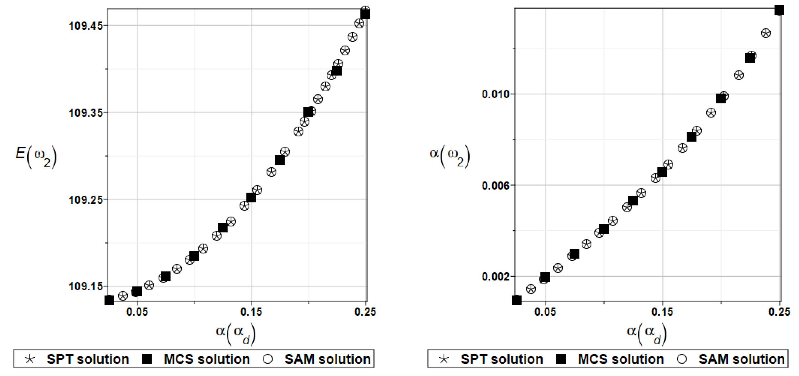
Figure 14.
Probabilistic moments for the second natural frequency and the random distribution of the damper’s material parameter αd.
Figure 14.
Probabilistic moments for the second natural frequency and the random distribution of the damper’s material parameter αd.
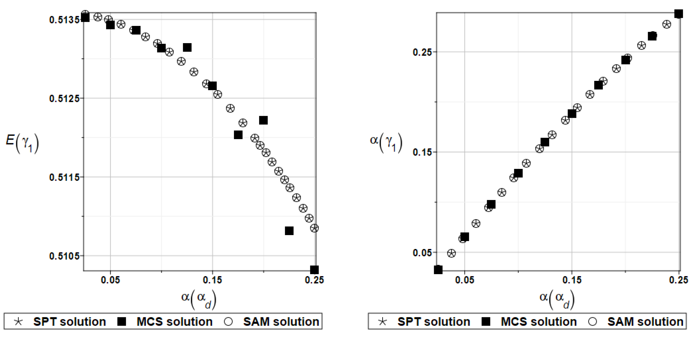
Figure 15.
Probabilistic moments for the coefficient of damping and the random distribution of the damper’s material parameter αd.
Figure 15.
Probabilistic moments for the coefficient of damping and the random distribution of the damper’s material parameter αd.
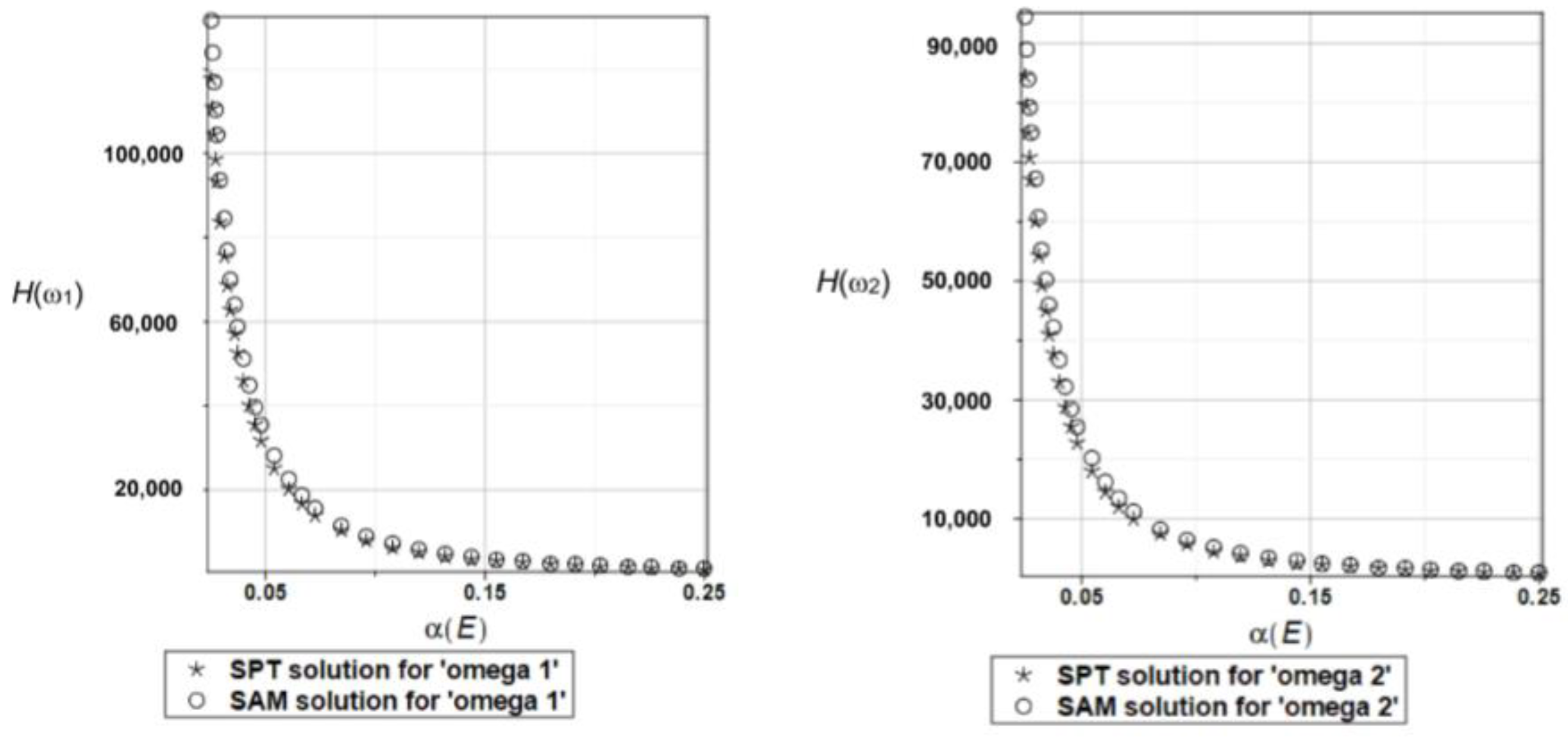
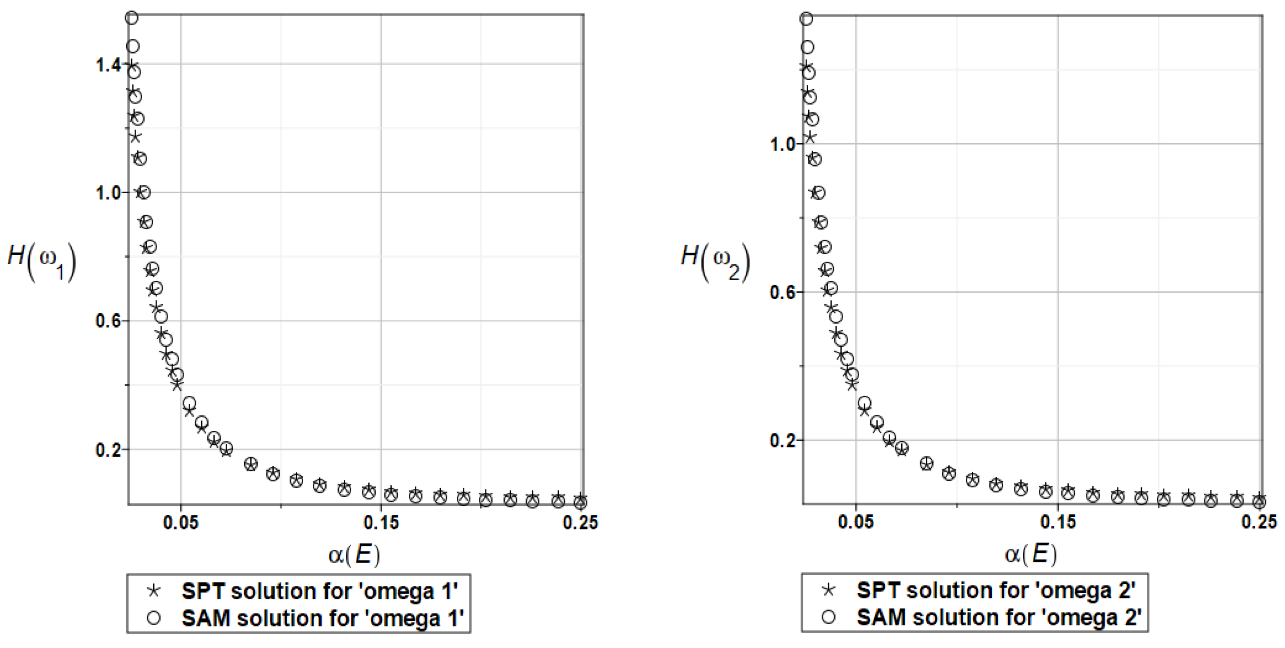
Figure 16.
The probabilistic relative entropy for the random distribution of Young’s modulus.
Figure 16.
The probabilistic relative entropy for the random distribution of Young’s modulus.
Figure 17.
The probabilistic safety measure for the random distribution of Young’s modulus.
Figure 17.
The probabilistic safety measure for the random distribution of Young’s modulus.
Figure 18.
Finite element mesh of the square isotropic plate simply supported on two opposite edges, with the remaining edges resting on viscoelastic constraints.
Figure 18.
Finite element mesh of the square isotropic plate simply supported on two opposite edges, with the remaining edges resting on viscoelastic constraints.
Figure 19.
Probabilistic moments for the first natural frequency and the random distribution of Young’s modulus.
Figure 19.
Probabilistic moments for the first natural frequency and the random distribution of Young’s modulus.
Figure 20.
Probabilistic moments for the first coefficient of damping and the random distribution of Young’s modulus.
Figure 20.
Probabilistic moments for the first coefficient of damping and the random distribution of Young’s modulus.
Figure 21.
Probabilistic moments for the third natural frequency and the random distribution of Poisson’s ratio.
Figure 21.
Probabilistic moments for the third natural frequency and the random distribution of Poisson’s ratio.
Figure 22.
Probabilistic moments for the third coefficient of damping and the random distribution of Poisson’s ratio.
Figure 22.
Probabilistic moments for the third coefficient of damping and the random distribution of Poisson’s ratio.
Figure 23.
Probabilistic moments for the first coefficient of damping and the random distribution of the damper’s parameter k1.
Figure 23.
Probabilistic moments for the first coefficient of damping and the random distribution of the damper’s parameter k1.
Figure 24.
Probabilistic moments for the first coefficient of damping and the random distribution of the damper’s parameter c1.
Figure 24.
Probabilistic moments for the first coefficient of damping and the random distribution of the damper’s parameter c1.
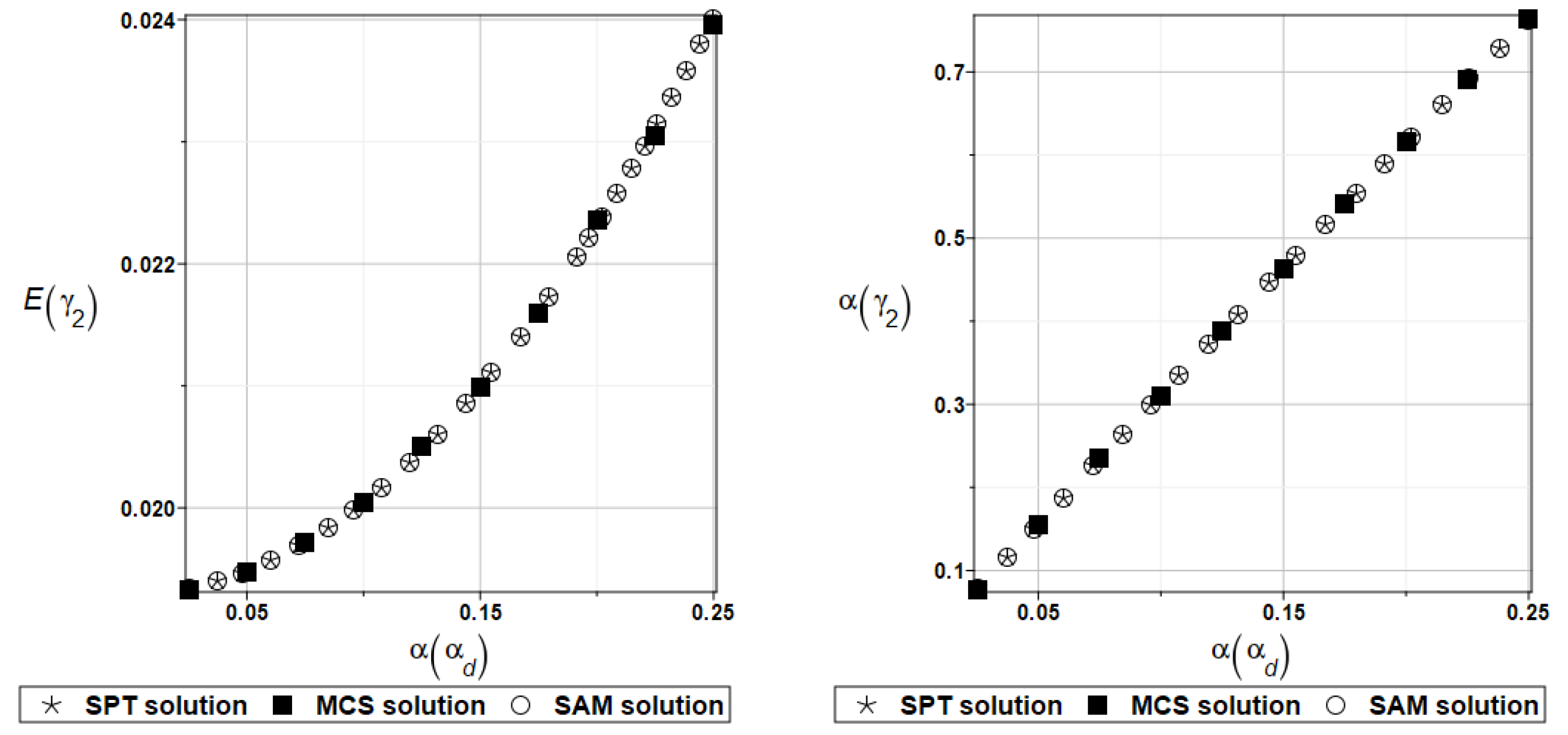
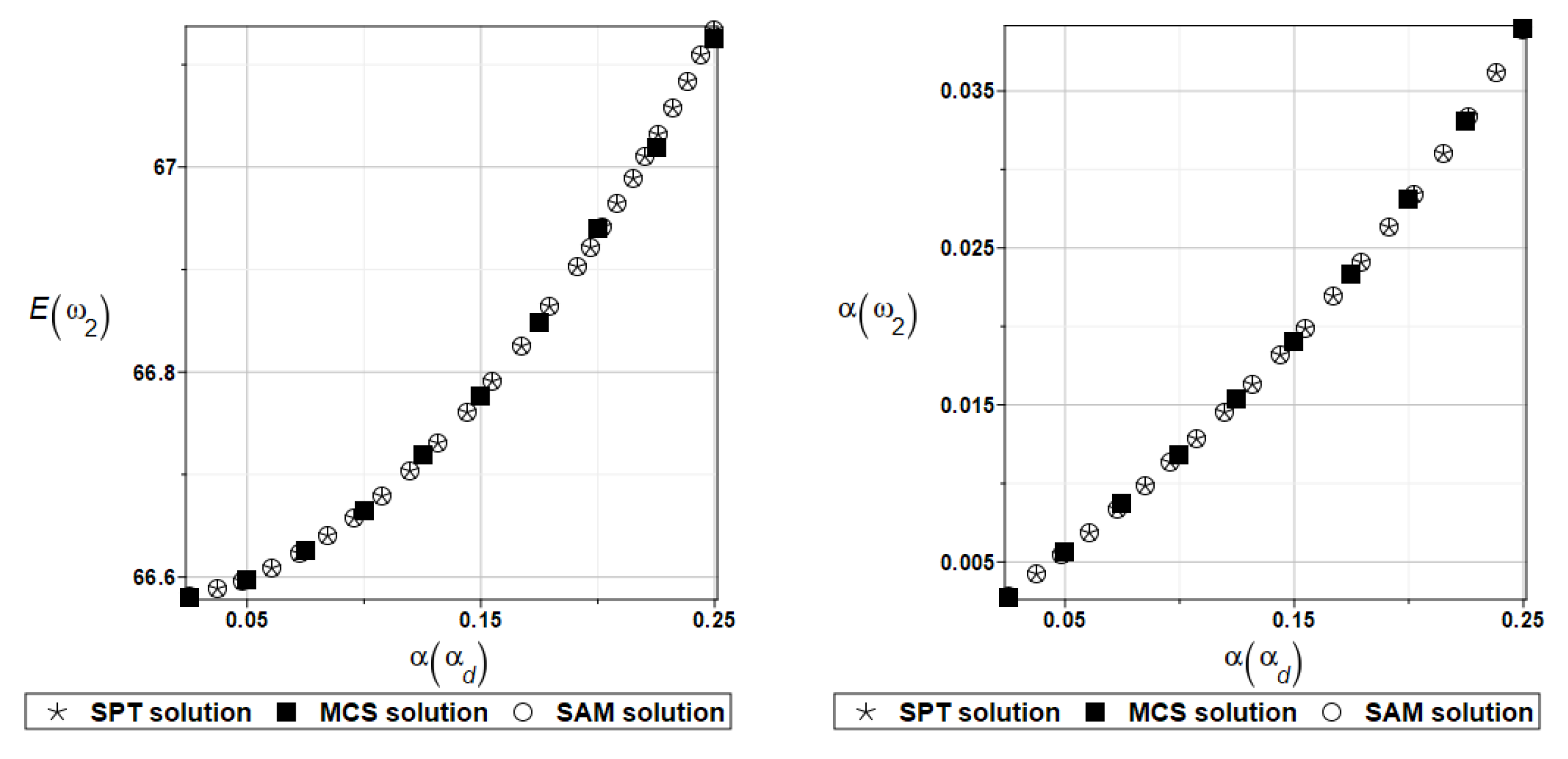
Figure 25.
Probabilistic moments for the second natural frequency and the random distribution of the damper’s material parameter αd.
Figure 25.
Probabilistic moments for the second natural frequency and the random distribution of the damper’s material parameter αd.
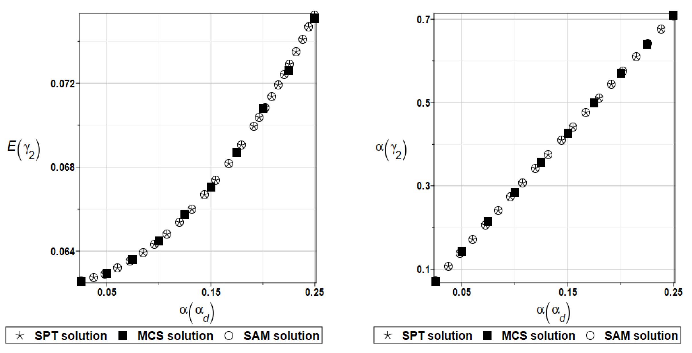
Figure 26.
Probabilistic moments for the second coefficient of damping and the random distribution of the damper’s material parameter αd.
Figure 26.
Probabilistic moments for the second coefficient of damping and the random distribution of the damper’s material parameter αd.
Figure 27.
The probabilistic relative entropy for the random distribution of Young’s modulus.
Figure 27.
The probabilistic relative entropy for the random distribution of Young’s modulus.
Figure 28.
The probabilistic safety measure for the random distribution of Young’s modulus.
Figure 28.
The probabilistic safety measure for the random distribution of Young’s modulus.
Figure 29.
Finite element mesh of the square isotropic plate resting on viscoelastic constraints placed along all edges.
Figure 29.
Finite element mesh of the square isotropic plate resting on viscoelastic constraints placed along all edges.
Figure 30.
Probabilistic moments for the third natural frequency and the random distribution of Young’s modulus.
Figure 30.
Probabilistic moments for the third natural frequency and the random distribution of Young’s modulus.
Figure 31.
Probabilistic moments for the third coefficient of damping and the random distribution of Young’s modulus.
Figure 31.
Probabilistic moments for the third coefficient of damping and the random distribution of Young’s modulus.
Figure 32.
Probabilistic moments for the third natural frequency and the random distribution of Poisson’s ratio.
Figure 32.
Probabilistic moments for the third natural frequency and the random distribution of Poisson’s ratio.
Figure 33.
Probabilistic moments for the third coefficient of damping and the random distribution of Poisson’s ratio.
Figure 33.
Probabilistic moments for the third coefficient of damping and the random distribution of Poisson’s ratio.
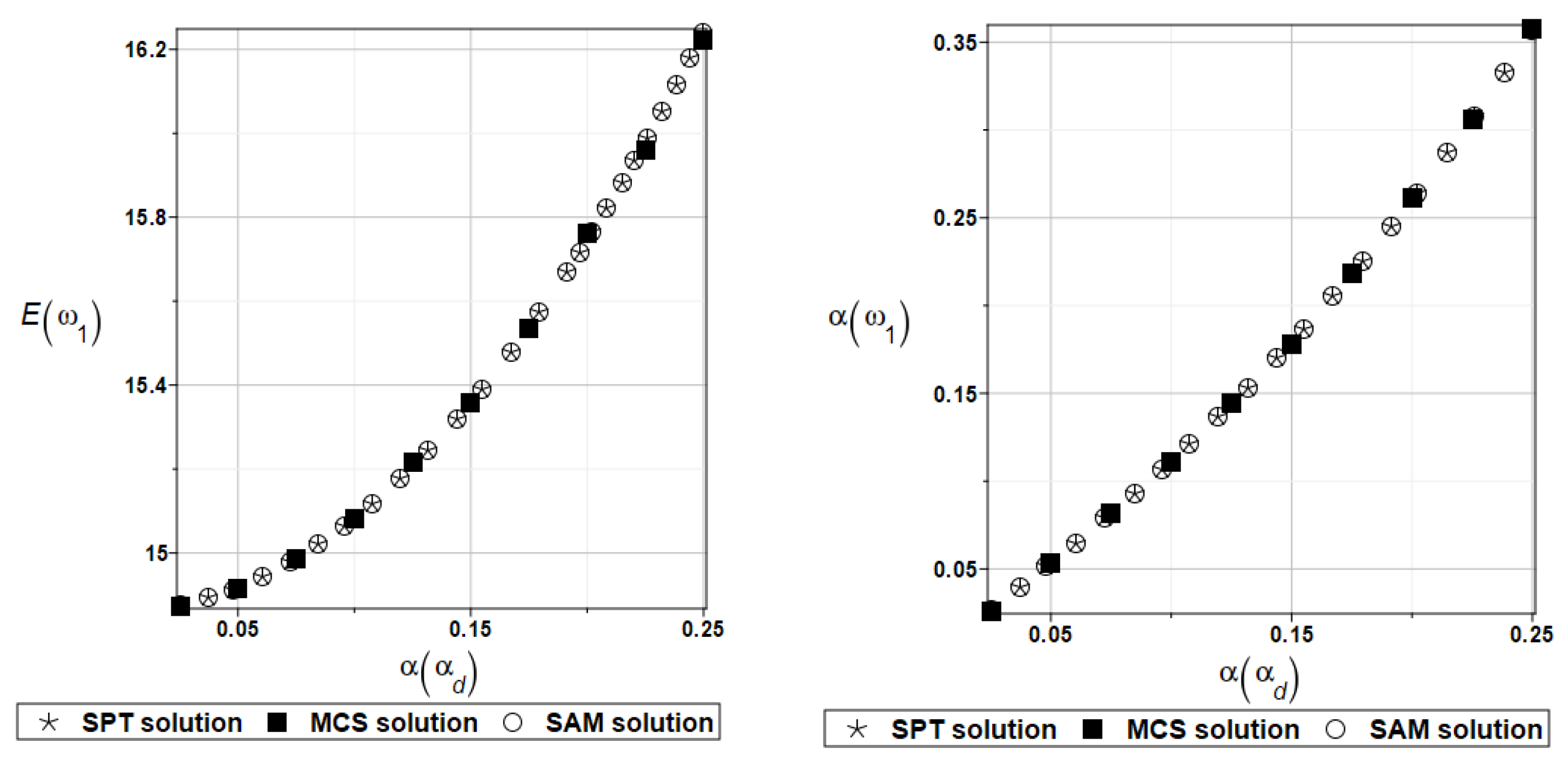
Figure 34.
Probabilistic moments for the first natural frequency and the random distribution of the damper’s material parameter αd.
Figure 34.
Probabilistic moments for the first natural frequency and the random distribution of the damper’s material parameter αd.
Figure 35.
Probabilistic moments for the first coefficient of damping and the random distribution of the damper’s material parameter αd.
Figure 35.
Probabilistic moments for the first coefficient of damping and the random distribution of the damper’s material parameter αd.
Figure 36.
The probabilistic relative entropy for the random distribution of the damper’s material parameter αd.
Figure 36.
The probabilistic relative entropy for the random distribution of the damper’s material parameter αd.
Figure 37.
The probabilistic safety measure for the random distribution of the damper’s material parameter αd.
Figure 37.
The probabilistic safety measure for the random distribution of the damper’s material parameter αd.
Table 1.
The results for the first four natural frequencies and the random distribution of Young’s modulus.
Table 1.
The results for the first four natural frequencies and the random distribution of Young’s modulus.
| E [GPa] | ω1 [rad/s] | ω2 [rad/s] | ω3 [rad/s] | ω4 [rad/s] |
|---|
| 180 | 44.7706 | 102.4523 | 150.7459 | 214.4013 |
| 185 | 45.3388 | 103.8232 | 152.7976 | 217.3323 |
| 190 | 45.8995 | 105.1760 | 154.8220 | 220.2242 |
| 195 | 46.4532 | 106.5113 | 156.8200 | 223.0783 |
| 200 | 47.0002 | 107.8302 | 158.7926 | 225.8963 |
| 205 | 47.5406 | 109.1326 | 160.7410 | 228.6793 |
| 210 | 48.0748 | 110.4194 | 162.6658 | 231.4287 |
| 215 | 48.6030 | 111.6911 | 164.5679 | 234.1457 |
| 220 | 49.1252 | 112.9483 | 166.4482 | 236.8314 |
| 225 | 49.6418 | 114.1916 | 168.3073 | 239.4868 |
| 230 | 50.1528 | 115.4212 | 170.1460 | 242.1130 |
Table 2.
The results for the first four coefficients of damping and the random distribution of Young’s modulus.
Table 2.
The results for the first four coefficients of damping and the random distribution of Young’s modulus.
| E [GPa] | γ1 [–] | γ2 [–] | γ3 [–] | γ4 [–] |
|---|
| 180 | 0.052066 | 0.021361 | 0.008305 | 0.005605 |
| 185 | 0.051161 | 0.020908 | 0.008139 | 0.005482 |
| 190 | 0.050291 | 0.020476 | 0.007981 | 0.005364 |
| 195 | 0.049454 | 0.020064 | 0.007829 | 0.005252 |
| 200 | 0.048650 | 0.019667 | 0.007683 | 0.005145 |
| 205 | 0.047875 | 0.019290 | 0.007544 | 0.005043 |
| 210 | 0.047129 | 0.018929 | 0.007410 | 0.004945 |
| 215 | 0.046410 | 0.018583 | 0.007281 | 0.004851 |
| 220 | 0.045716 | 0.018251 | 0.007157 | 0.004761 |
| 225 | 0.045045 | 0.017931 | 0.007038 | 0.004674 |
| 230 | 0.044397 | 0.017624 | 0.006923 | 0.004591 |
Table 3.
The results for the first four natural frequencies and the random distribution of Poisson’s ratio.
Table 3.
The results for the first four natural frequencies and the random distribution of Poisson’s ratio.
| V [–] | ω1 [rad/s] | ω2 [rad/s] | ω3 [rad/s] | ω4 [rad/s] |
|---|
| 0.25 | 47.2828 | 108.4706 | 159.0997 | 226.7159 |
| 0.26 | 47.3295 | 108.5801 | 159.4025 | 227.0638 |
| 0.27 | 47.3786 | 108.7008 | 159.7179 | 227.4336 |
| 0.28 | 47.4302 | 108.8332 | 160.0461 | 227.8258 |
| 0.29 | 47.4842 | 108.9769 | 160.3871 | 228.2409 |
| 0.30 | 47.5406 | 109.1326 | 160.7410 | 228.6793 |
| 0.31 | 47.5996 | 109.3004 | 161.1078 | 229.1417 |
| 0.32 | 47.6609 | 109.4808 | 161.4877 | 229.6286 |
| 0.33 | 47.7246 | 109.6741 | 161.8808 | 230.1408 |
| 0.34 | 47.7907 | 109.8805 | 162.2872 | 230.6790 |
| 0.35 | 47.8594 | 110.1006 | 162.7068 | 231.2439 |
Table 4.
The results for the first four coefficients of damping and the random distribution of Poisson’s ratio.
Table 4.
The results for the first four coefficients of damping and the random distribution of Poisson’s ratio.
| V [–] | γ1 [–] | γ2 [–] | γ3 [–] | γ4 [–] |
|---|
| 0.25 | 0.046118 | 0.019375 | 0.007118 | 0.004985 |
| 0.26 | 0.046461 | 0.019367 | 0.007198 | 0.004999 |
| 0.27 | 0.046808 | 0.019354 | 0.007281 | 0.005012 |
| 0.28 | 0.047160 | 0.019337 | 0.007366 | 0.005024 |
| 0.29 | 0.047516 | 0.019316 | 0.007454 | 0.005034 |
| 0.30 | 0.047875 | 0.019290 | 0.007544 | 0.005043 |
| 0.31 | 0.048240 | 0.019260 | 0.007637 | 0.005050 |
| 0.32 | 0.048610 | 0.019224 | 0.007732 | 0.005056 |
| 0.33 | 0.048984 | 0.019183 | 0.007831 | 0.005059 |
| 0.34 | 0.049363 | 0.019137 | 0.007932 | 0.005061 |
| 0.35 | 0.049748 | 0.019086 | 0.008036 | 0.005062 |
Table 5.
The results for the first four natural frequencies and the random distribution of damper’s parameter k0.
Table 5.
The results for the first four natural frequencies and the random distribution of damper’s parameter k0.
| K0 [N/m] | ω1 [rad/s] | ω2 [rad/s] | ω3 [rad/s] | ω4 [rad/s] |
|---|
| 95 | 47.5200 | 109.1197 | 160.7347 | 228.6742 |
| 98 | 47.5241 | 109.1223 | 160.7360 | 228.6752 |
| 101 | 47.5283 | 109.1248 | 160.7372 | 228.6762 |
| 104 | 47.5324 | 109.1274 | 160.7385 | 228.6772 |
| 107 | 47.5365 | 109.1300 | 160.7397 | 228.6783 |
| 110 | 47.5406 | 109.1326 | 160.7410 | 228.6793 |
| 113 | 47.5448 | 109.1351 | 160.7422 | 228.6803 |
| 116 | 47.5489 | 109.1377 | 160.7435 | 228.6814 |
| 119 | 47.5531 | 109.1403 | 160.7447 | 228.6824 |
| 122 | 47.5572 | 109.1429 | 160.7459 | 228.6834 |
| 125 | 47.5612 | 109.1454 | 160.7472 | 228.6845 |
Table 6.
The results for the first four coefficients of damping and the random distribution of the damper’s parameter k0.
Table 6.
The results for the first four coefficients of damping and the random distribution of the damper’s parameter k0.
| K0 [N/m] | γ1 [–] | γ2 [–] | γ3 [–] | γ4 [–] |
|---|
| 95 | 0.047944 | 0.019290 | 0.007546 | 0.005043 |
| 98 | 0.047931 | 0.019290 | 0.007546 | 0.005043 |
| 101 | 0.047917 | 0.019290 | 0.007545 | 0.005043 |
| 104 | 0.047903 | 0.019290 | 0.007545 | 0.005043 |
| 107 | 0.047889 | 0.019290 | 0.007544 | 0.005043 |
| 110 | 0.047875 | 0.019290 | 0.007544 | 0.005043 |
| 113 | 0.047862 | 0.019290 | 0.007543 | 0.005043 |
| 116 | 0.047848 | 0.019290 | 0.007543 | 0.005043 |
| 119 | 0.047834 | 0.019290 | 0.007542 | 0.005043 |
| 122 | 0.047821 | 0.019291 | 0.007542 | 0.005043 |
| 125 | 0.047807 | 0.019291 | 0.007541 | 0.005043 |
Table 7.
The results for the first four natural frequencies and the random distribution of the damper’s parameter k1.
Table 7.
The results for the first four natural frequencies and the random distribution of the damper’s parameter k1.
| K1 [N/m] | ω1 [rad/s] | ω2 [rad/s] | ω3 [rad/s] | ω4 [rad/s] |
|---|
| 17,500 | 47.5417 | 109.1356 | 160.7358 | 228.6728 |
| 18,000 | 47.5415 | 109.1351 | 160.7371 | 228.6744 |
| 18,500 | 47.5414 | 109.1346 | 160.7382 | 228.6759 |
| 19,000 | 47.5411 | 109.1340 | 160.7393 | 228.6772 |
| 19,500 | 47.5410 | 109.1333 | 160.7402 | 228.6783 |
| 20,000 | 47.5406 | 109.1326 | 160.7410 | 228.6793 |
| 20,500 | 47.5404 | 109.1318 | 160.7417 | 228.6802 |
| 21,000 | 47.5400 | 109.1310 | 160.7423 | 228.6809 |
| 21,500 | 47.5397 | 109.1301 | 160.7428 | 228.6815 |
| 22,000 | 47.5394 | 109.1292 | 160.7433 | 228.6821 |
| 22,500 | 47.5391 | 109.1283 | 160.7437 | 228.6826 |
Table 8.
The results for the first four coefficients of damping and the random distribution of the damper’s parameter k1.
Table 8.
The results for the first four coefficients of damping and the random distribution of the damper’s parameter k1.
| K1 [N/m] | γ1 [–] | γ2 [–] | γ3 [–] | γ4 [–] |
|---|
| 17,500 | 0.046892 | 0.018644 | 0.007229 | 0.004784 |
| 18,000 | 0.047109 | 0.018786 | 0.007298 | 0.004840 |
| 18,500 | 0.047315 | 0.018921 | 0.007363 | 0.004894 |
| 19,000 | 0.047511 | 0.019050 | 0.007426 | 0.004946 |
| 19,500 | 0.047698 | 0.019173 | 0.007486 | 0.004995 |
| 20,000 | 0.047875 | 0.019290 | 0.007544 | 0.005043 |
| 20,500 | 0.048046 | 0.019403 | 0.007599 | 0.005088 |
| 21,000 | 0.048208 | 0.019510 | 0.007652 | 0.005132 |
| 21,500 | 0.048363 | 0.019614 | 0.007703 | 0.005175 |
| 22,000 | 0.048512 | 0.019713 | 0.007752 | 0.005215 |
| 22,500 | 0.048654 | 0.019808 | 0.007799 | 0.005254 |
Table 9.
The results for the first four natural frequencies and random distribution of the damper’s parameter c1.
Table 9.
The results for the first four natural frequencies and random distribution of the damper’s parameter c1.
| C1 [N·s/m] | ω1 [rad/s] | ω2 [rad/s] | ω3 [rad/s] | ω4 [rad/s] |
|---|
| 205 | 47.2923 | 108.9110 | 160.5999 | 228.5450 |
| 210 | 47.3419 | 108.9552 | 160.6283 | 228.5721 |
| 215 | 47.3915 | 108.9995 | 160.6566 | 228.5990 |
| 220 | 47.4413 | 109.0439 | 160.6848 | 228.6258 |
| 225 | 47.4910 | 109.0882 | 160.7129 | 228.6526 |
| 230 | 47.5406 | 109.1326 | 160.7410 | 228.6793 |
| 235 | 47.5904 | 109.1769 | 160.7689 | 228.7059 |
| 240 | 47.6401 | 109.2209 | 160.7968 | 228.7324 |
| 245 | 47.6899 | 109.2653 | 160.8245 | 228.7588 |
| 250 | 47.7397 | 109.3096 | 160.8522 | 228.7851 |
| 255 | 47.7895 | 109.3540 | 160.8798 | 228.8114 |
Table 10.
The results for the first four coefficients of damping and the random distribution of the damper’s parameter c1.
Table 10.
The results for the first four coefficients of damping and the random distribution of the damper’s parameter c1.
| C1 [N·s/m] | γ1 [–] | γ2 [–] | γ3 [–] | γ4 [–] |
|---|
| 205 | 0.043901 | 0.017609 | 0.006994 | 0.004676 |
| 210 | 0.044718 | 0.017953 | 0.007108 | 0.004753 |
| 215 | 0.045524 | 0.018293 | 0.007220 | 0.004827 |
| 220 | 0.046319 | 0.018629 | 0.007330 | 0.004901 |
| 225 | 0.047103 | 0.018962 | 0.007438 | 0.004972 |
| 230 | 0.047875 | 0.019290 | 0.007544 | 0.005043 |
| 235 | 0.048638 | 0.019615 | 0.007647 | 0.005112 |
| 240 | 0.049389 | 0.019939 | 0.007749 | 0.005179 |
| 245 | 0.050129 | 0.020256 | 0.007848 | 0.005246 |
Table 11.
The results for the first four natural frequencies and the random distribution of the damper’s material parameter αd.
Table 11.
The results for the first four natural frequencies and the random distribution of the damper’s material parameter αd.
| αd [–] | ω1 [rad/s] | ω2 [rad/s] | ω3 [rad/s] | ω4 [rad/s] |
|---|
| 0.50 | 47.0136 | 108.5517 | 160.3107 | 228.2408 |
| 0.52 | 47.1075 | 108.6520 | 160.3828 | 228.3133 |
| 0.54 | 47.2065 | 108.7594 | 160.4612 | 228.3925 |
| 0.56 | 47.3112 | 108.8746 | 160.5464 | 228.4793 |
| 0.58 | 47.4223 | 108.9986 | 160.6393 | 228.5745 |
| 0.60 | 47.5406 | 109.1326 | 160.7410 | 228.6793 |
| 0.62 | 47.6672 | 109.2774 | 160.8525 | 228.7950 |
| 0.64 | 47.8032 | 109.4356 | 160.9752 | 228.9230 |
Table 12.
The results for the first four coefficients of damping and the random distribution of the damper’s material parameter αd.
Table 12.
The results for the first four coefficients of damping and the random distribution of the damper’s material parameter αd.
| αd [–] | γ1 [–] | γ2 [–] | γ3 [–] | γ4 [–] |
|---|
| 0.50 | 0.029935 | 0.011166 | 0.004429 | 0.002886 |
| 0.52 | 0.033009 | 0.012512 | 0.004959 | 0.003249 |
| 0.54 | 0.036325 | 0.013988 | 0.005534 | 0.003646 |
| 0.56 | 0.039898 | 0.015604 | 0.006156 | 0.004077 |
| 0.58 | 0.043743 | 0.017368 | 0.006826 | 0.004543 |
| 0.60 | 0.047875 | 0.019290 | 0.007544 | 0.005043 |
| 0.62 | 0.052313 | 0.021384 | 0.008309 | 0.005576 |
| 0.64 | 0.057071 | 0.023653 | 0.009119 | 0.006141 |
| 0.66 | 0.062168 | 0.026109 | 0.009969 | 0.006733 |
| 0.68 | 0.067617 | 0.028761 | 0.010855 | 0.007347 |
| 0.70 | 0.073437 | 0.031612 | 0.011767 | 0.007974 |
Table 13.
The results for the first four natural frequencies and the random distribution of Young’s modulus.
Table 13.
The results for the first four natural frequencies and the random distribution of Young’s modulus.
| E [GPa] | ω1 [rad/s] | ω2 [rad/s] | ω3 [rad/s] | ω4 [rad/s] |
|---|
| 180 | 37.1491 | 62.7840 | 136.4726 | 142.6124 |
| 185 | 37.6159 | 63.5616 | 138.2809 | 144.5536 |
| 190 | 38.0767 | 64.3293 | 140.0650 | 146.4688 |
| 195 | 38.5318 | 65.0877 | 141.8260 | 148.3591 |
| 200 | 38.9814 | 65.8369 | 143.5655 | 150.2255 |
| 205 | 39.4257 | 66.5773 | 145.2833 | 152.0689 |
| 210 | 39.8648 | 67.3093 | 146.9808 | 153.8900 |
| 215 | 40.2990 | 68.0330 | 148.6586 | 155.6896 |
| 220 | 40.7283 | 68.7489 | 150.3176 | 157.4686 |
| 225 | 41.1531 | 69.4570 | 151.9577 | 159.2275 |
| 230 | 41.5733 | 70.1577 | 153.5803 | 160.9671 |
Table 14.
The results for the first four coefficients of damping and the random distribution of Young’s modulus.
Table 14.
The results for the first four coefficients of damping and the random distribution of Young’s modulus.
| E [GPa] | γ1 [–] | γ2 [–] | γ3 [–] | γ4 [–] |
|---|
| 180 | 0.059028 | 0.068283 | 0.026588 | 0.008418 |
| 185 | 0.057991 | 0.067014 | 0.026025 | 0.008249 |
| 190 | 0.056991 | 0.065799 | 0.025490 | 0.008087 |
| 195 | 0.056039 | 0.064633 | 0.024980 | 0.007932 |
| 200 | 0.055120 | 0.063515 | 0.024490 | 0.007783 |
| 205 | 0.054235 | 0.062440 | 0.024023 | 0.007641 |
| 210 | 0.053383 | 0.061407 | 0.023575 | 0.007504 |
| 215 | 0.052562 | 0.060412 | 0.023144 | 0.007373 |
| 220 | 0.051770 | 0.059455 | 0.022730 | 0.007247 |
| 225 | 0.051005 | 0.058531 | 0.022334 | 0.007125 |
| 230 | 0.050267 | 0.057640 | 0.021951 | 0.007008 |
Table 15.
The results for the first four natural frequencies and the random distribution of Poisson’s ratio.
Table 15.
The results for the first four natural frequencies and the random distribution of Poisson’s ratio.
| V [–] | ω1 [rad/s] | ω2 [rad/s] | ω3 [rad/s] | ω4 [rad/s] |
|---|
| 0.25 | 39.0949 | 66.9109 | 144.9199 | 150.4124 |
| 0.26 | 39.1571 | 66.8397 | 144.9639 | 150.7189 |
| 0.27 | 39.2213 | 66.7707 | 145.0217 | 151.0376 |
| 0.28 | 39.2874 | 66.7040 | 145.0944 | 151.3688 |
| 0.29 | 39.3555 | 66.6396 | 145.1812 | 151.7125 |
| 0.30 | 39.4257 | 66.5773 | 145.2833 | 152.0689 |
| 0.31 | 39.4978 | 66.5172 | 145.4009 | 152.4380 |
| 0.32 | 39.5719 | 66.4593 | 145.5336 | 152.8202 |
| 0.33 | 39.6480 | 66.4034 | 145.6829 | 153.2154 |
| 0.34 | 39.7262 | 66.3496 | 145.8481 | 153.6238 |
| 0.35 | 39.8064 | 66.2978 | 146.0307 | 154.0456 |
Table 16.
The results for the first four coefficients of damping and the random distribution of Poisson’s ratio.
Table 16.
The results for the first four coefficients of damping and the random distribution of Poisson’s ratio.
| V [–] | γ1 [–] | γ2 [–] | γ3 [–] | γ4 [–] |
|---|
| 0.25 | 0.052825 | 0.060718 | 0.024053 | 0.007281 |
| 0.26 | 0.053101 | 0.061062 | 0.024056 | 0.007349 |
| 0.27 | 0.053380 | 0.061407 | 0.024056 | 0.007419 |
| 0.28 | 0.053662 | 0.061751 | 0.024048 | 0.007491 |
| 0.29 | 0.053947 | 0.062096 | 0.024039 | 0.007565 |
| 0.30 | 0.054235 | 0.062440 | 0.024023 | 0.007641 |
| 0.31 | 0.054526 | 0.062785 | 0.024001 | 0.007719 |
| 0.32 | 0.054821 | 0.063130 | 0.023977 | 0.007799 |
| 0.33 | 0.055119 | 0.063475 | 0.023945 | 0.007881 |
| 0.34 | 0.055422 | 0.063820 | 0.023910 | 0.007965 |
| 0.35 | 0.055727 | 0.064166 | 0.023867 | 0.008051 |
Table 17.
The results for the first four natural frequencies and the random distribution of the damper’s parameter k0.
Table 17.
The results for the first four natural frequencies and the random distribution of the damper’s parameter k0.
| K0 [N/m] | ω1 [rad/s] | ω2 [rad/s] | ω3 [rad/s] | ω4 [rad/s] |
|---|
| 95 | 39.4043 | 66.5454 | 145.2648 | 152.0628 |
| 98 | 39.4086 | 66.5518 | 145.2685 | 152.0640 |
| 101 | 39.4129 | 66.5582 | 145.2723 | 152.0652 |
| 104 | 39.4171 | 66.5646 | 145.2760 | 152.0664 |
| 107 | 39.4214 | 66.5710 | 145.2798 | 152.0676 |
Table 18.
The results for the first four coefficients of damping and the random distribution of the damper’s parameter k0.
Table 18.
The results for the first four coefficients of damping and the random distribution of the damper’s parameter k0.
| K0 [N/m] | γ1 [–] | γ2 [–] | γ3 [–] | γ4 [–] |
|---|
| 95 | 0.054315 | 0.062498 | 0.024024 | 0.007643 |
| 98 | 0.054299 | 0.062487 | 0.024024 | 0.007643 |
| 101 | 0.054283 | 0.062475 | 0.024023 | 0.007642 |
| 104 | 0.054267 | 0.062463 | 0.024023 | 0.007642 |
| 107 | 0.054251 | 0.062452 | 0.024022 | 0.007641 |
Table 19.
The results for the first four natural frequencies and the random distribution of the damper’s parameter k1.
Table 19.
The results for the first four natural frequencies and the random distribution of the damper’s parameter k1.
| K1 [N/m] | ω1 [rad/s] | ω2 [rad/s] | ω3 [rad/s] | ω4 [rad/s] |
|---|
| 17,500 | 39.4280 | 66.5811 | 145.2801 | 152.0650 |
| 18,000 | 39.4276 | 66.5805 | 145.2812 | 152.0660 |
| 18,500 | 39.4271 | 66.5798 | 145.2824 | 152.0669 |
| 19,000 | 39.4266 | 66.5791 | 145.2830 | 152.0676 |
| 19,500 | 39.4262 | 66.5782 | 145.2834 | 152.0683 |
Table 20.
The results for the first four coefficients of damping and the random distribution of the damper’s parameter k1.
Table 20.
The results for the first four coefficients of damping and the random distribution of the damper’s parameter k1.
| K1 [N/m] | γ1 [–] | γ2 [–] | γ3 [–] | γ4 [–] |
|---|
| 17,500 | 0.053241 | 0.060875 | 0.023070 | 0.007332 |
| 18,000 | 0.053460 | 0.061220 | 0.023279 | 0.007399 |
| 18,500 | 0.053669 | 0.061547 | 0.023476 | 0.007464 |
| 19,000 | 0.053866 | 0.061859 | 0.023666 | 0.007525 |
| 19,500 | 0.054055 | 0.062157 | 0.023848 | 0.007584 |
Table 21.
The results for the first four natural frequencies and the random distribution of the damper’s parameter c1.
Table 21.
The results for the first four natural frequencies and the random distribution of the damper’s parameter c1.
| C1 [N·s/m] | ω1 [rad/s] | ω2 [rad/s] | ω3 [rad/s] | ω4 [rad/s] |
|---|
| 205 | 39.1985 | 66.1265 | 144.8963 | 151.9355 |
| 210 | 39.2438 | 66.2165 | 144.9740 | 151.9623 |
| 215 | 39.2892 | 66.3066 | 145.0515 | 151.9891 |
| 220 | 39.3346 | 66.3967 | 145.1286 | 152.0157 |
| 225 | 39.3801 | 66.4870 | 145.2062 | 152.0423 |
Table 22.
The results for the first four coefficients of damping and the random distribution of the damper’s parameter c1.
Table 22.
The results for the first four coefficients of damping and the random distribution of the damper’s parameter c1.
| C1 [N·s/m] | γ1 [–] | γ2 [–] | γ3 [–] | γ4 [–] |
|---|
| 205 | 0.049568 | 0.057213 | 0.022088 | 0.007068 |
| 210 | 0.050524 | 0.058287 | 0.022486 | 0.007187 |
| 215 | 0.051468 | 0.059346 | 0.022879 | 0.007304 |
| 220 | 0.052402 | 0.060392 | 0.023267 | 0.007418 |
| 225 | 0.053324 | 0.061423 | 0.023647 | 0.007531 |
Table 23.
The results for the first four natural frequencies and the random distribution of the damper’s material parameter αd.
Table 23.
The results for the first four natural frequencies and the random distribution of the damper’s material parameter αd.
| αd [–] | ω1 [rad/s] | ω2 [rad/s] | ω3 [rad/s] | ω4 [rad/s] |
|---|
| 0.50 | 38.9825 | 65.5297 | 144.1695 | 151.6698 |
| 0.52 | 39.0628 | 65.7132 | 144.3574 | 151.7370 |
| 0.54 | 39.1469 | 65.9082 | 144.5607 | 151.8098 |
| 0.56 | 39.2351 | 66.1161 | 144.7811 | 151.8888 |
| 0.58 | 39.3278 | 66.3385 | 145.0212 | 151.9749 |
| 0.60 | 39.4257 | 66.5773 | 145.2833 | 152.0689 |
| 0.62 | 39.5293 | 66.8349 | 145.5714 | 152.1719 |
| 0.64 | 39.6393 | 67.1142 | 145.8882 | 152.2851 |
| 0.66 | 39.7569 | 67.4187 | 146.2393 | 152.4098 |
| 0.68 | 39.8831 | 67.7527 | 146.6298 | 152.5474 |
| 0.70 | 40.0195 | 68.1218 | 147.0659 | 152.6997 |
Table 24.
The results for the first four coefficients of damping and the random distribution of the damper’s material parameter αd.
Table 24.
The results for the first four coefficients of damping and the random distribution of the damper’s material parameter αd.
| αd [–] | γ1 [–] | γ2 [–] | γ3 [–] | γ4 [–] |
|---|
| 0.50 | 0.034187 | 0.037911 | 0.013852 | 0.004476 |
| 0.52 | 0.037626 | 0.042057 | 0.015548 | 0.005011 |
| 0.54 | 0.041332 | 0.046559 | 0.017403 | 0.005594 |
| 0.56 | 0.045323 | 0.051441 | 0.019429 | 0.006226 |
| 0.58 | 0.049617 | 0.056726 | 0.021632 | 0.006908 |
| 0.60 | 0.054235 | 0.062440 | 0.024023 | 0.007641 |
| 0.62 | 0.059197 | 0.068610 | 0.026604 | 0.008425 |
| 0.64 | 0.064525 | 0.075263 | 0.029385 | 0.009258 |
| 0.66 | 0.070243 | 0.082423 | 0.032360 | 0.010137 |
| 0.68 | 0.076376 | 0.090117 | 0.035527 | 0.011059 |
| 0.70 | 0.082951 | 0.098368 | 0.038877 | 0.012016 |
Table 25.
The results for the first four natural frequencies and the random distribution of Young’s modulus.
Table 25.
The results for the first four natural frequencies and the random distribution of Young’s modulus.
| E [GPa] | ω1 [rad/s] | ω2 [rad/s] | ω3 [rad/s] | ω4 [rad/s] |
|---|
| 180 | 14.8318 | 24.4221 | 58.0999 | 78.2479 |
| 185 | 14.8393 | 24.4260 | 58.7038 | 79.1780 |
| 190 | 14.8464 | 24.4292 | 59.3013 | 80.0965 |
| 195 | 14.8532 | 24.4319 | 59.8924 | 81.0043 |
| 200 | 14.8596 | 24.4350 | 60.4776 | 81.9014 |
Table 26.
The results for the first four coefficients of damping and the random distribution of Young’s modulus.
Table 26.
The results for the first four coefficients of damping and the random distribution of Young’s modulus.
| E [Gpa] | γ1 [–] | γ2 [–] | γ3 [–] | γ4 [–] |
|---|
| 180 | 0.509837 | 0.533552 | 0.152404 | 0.090064 |
| 185 | 0.510657 | 0.533790 | 0.149889 | 0.088395 |
| 190 | 0.511434 | 0.534026 | 0.147469 | 0.086796 |
| 195 | 0.512173 | 0.534264 | 0.145139 | 0.085262 |
| 200 | 0.512876 | 0.534475 | 0.142893 | 0.083790 |
Table 27.
The results for the first four natural frequencies and the random distribution of Poisson’s ratio.
Table 27.
The results for the first four natural frequencies and the random distribution of Poisson’s ratio.
| v [–] | ω1 [rad/s] | ω2 [rad/s] | ω3 [rad/s] | ω4 [rad/s] |
|---|
| 0.25 | 14.8509 | 24.4341 | 61.8065 | 83.6013 |
| 0.26 | 14.8539 | 24.4350 | 61.6526 | 83.4333 |
| 0.27 | 14.8568 | 24.4358 | 61.5008 | 83.2680 |
| 0.28 | 14.8597 | 24.4358 | 61.3508 | 83.1054 |
| 0.29 | 14.8627 | 24.4369 | 61.2029 | 82.9455 |
Table 28.
The results for the first four coefficients of damping and the random distribution of Poisson’s ratio.
Table 28.
The results for the first four coefficients of damping and the random distribution of Poisson’s ratio.
| v [–] | γ1 [–] | γ2 [–] | γ3 [–] | γ4 [–] |
|---|
| 0.25 | 0.511905 | 0.534396 | 0.136860 | 0.080368 |
| 0.26 | 0.512231 | 0.534441 | 0.137637 | 0.080772 |
| 0.27 | 0.512558 | 0.534496 | 0.138412 | 0.081174 |
| 0.28 | 0.512886 | 0.534525 | 0.139185 | 0.081575 |
Table 29.
The results for the first four natural frequencies and the random distribution of the damper’s material parameter αd.
Table 29.
The results for the first four natural frequencies and the random distribution of the damper’s material parameter αd.
| αd [–] | ω1 [rad/s] | ω2 [rad/s] | ω3 [rad/s] | ω4 [rad/s] |
|---|
| 0.50 | 12.7353 | 20.1901 | 58.7623 | 80.8862 |
| 0.52 | 13.0975 | 20.9059 | 59.1553 | 81.2122 |
| 0.54 | 13.4877 | 21.6804 | 59.5769 | 81.5621 |
| 0.56 | 13.9095 | 22.5215 | 60.0309 | 81.9388 |
| 0.58 | 14.3672 | 23.4371 | 60.5222 | 82.3461 |
| 0.60 | 14.8656 | 24.4378 | 61.0567 | 82.7882 |
Table 30.
The results for the first four coefficients of damping and the random distribution of the damper’s material parameter αd.
Table 30.
The results for the first four coefficients of damping and the random distribution of the damper’s material parameter αd.
| αd [–] | γ1 [–] | γ2 [–] | γ3 [–] | γ4 [–] |
|---|
| 0.50 | 0.401650 | 0.420408 | 0.087266 | 0.049563 |
| 0.52 | 0.423633 | 0.443153 | 0.096394 | 0.055101 |
| 0.54 | 0.445879 | 0.466047 | 0.106259 | 0.061121 |
| 0.56 | 0.468353 | 0.488975 | 0.116905 | 0.067653 |
| 0.58 | 0.490930 | 0.511909 | 0.128378 | 0.074727 |


 ,
, 


