Article

General Planar Ideal Flow Solutions with No Symmetry Axis

by
Sergei Alexandrov
1,2 and
Vyacheslav Mokryakov
1,*
1
Ishlinsky Institute for Problems in Mechanics RAS, 101-1 Prospect Vernadskogo, Moscow 119526, Russia
2
Department of Civil Engineering, RUDN University, 6 Miklukho-Maklaya St., Moscow 117198, Russia
*
Author to whom correspondence should be addressed.
Materials 2023, 16(23), 7378; https://doi.org/10.3390/ma16237378
Submission received: 27 October 2023 / Revised: 23 November 2023 / Accepted: 24 November 2023 / Published: 27 November 2023
(This article belongs to the Special Issue Sheet/Bulk Metal Forming and Hybrid Components: Theory and Experiment)

Abstract

:
Bulk ideal flows constitute a wide class of solutions in plasticity theory. Ideal flow solutions concern inverse problems. In particular, the solution determines part of the boundary of a region where it is valid. Bulk planar ideal flows exist in the case of (i) isotropic rigid/plastic material obeying an arbitrary pressure-independent yield criterion and its associated flow rule and (ii) the double sliding and rotation model based on the Mohr–Coulomb yield criterion. In the latter case, the intrinsic spin must vanish. Both models are perfectly plastic, and the complete equation systems are hyperbolic. All available specific solutions for both models describe flows with a symmetry axis. The present paper aims at general solutions for flows with no symmetry axis. The general structure of the solutions consists of two rigid regions connected by a plastic region. The characteristic lines between the plastic and rigid regions must be straight, which partly dictates the general structure of the characteristic nets. The solutions employ Riemann’s method in regions where the characteristics of both families are curvilinear. Special solutions that do not have such regions are considered separately. In any case, the solutions are practically analytical. A numerical technique is only necessary to evaluate ordinary integrals. The solutions found determine the tool shapes that produce ideal flows. In addition, the distribution of pressure over the tool’s surface is calculated, which is important for predicting the wear of tools.

1. Introduction

Ideal or streamlined flows constitute a class of solutions within the classical theory of rigid plasticity. The ideal flow condition is an additional equation within the standard system of equations of the latterly mentioned theory. Nevertheless, the resulting overdetermined system of equations is compatible, and restrictions are imposed on boundary conditions. Ideal flow solutions are design solutions. In particular, in the case of bulk stationary flows, a tool’s shape is not a given but is partly determined by the solution [1]. The first design solution of this kind has been presented in [2]. It was based on the method of characteristics. The traditional finite element method cannot calculate ideal flows. An ideal flow condition is advantageous for some deformation processes. In particular, ideal flows produce no redundant work [2]. This work is not zero in real processes. However, the experiment carried out in [3] has demonstrated that the ideal-flow die calculated in [2] is the best in terms of the following criteria: efficiency, uniformity of deformation, product strength, ductility, and fatigue life. This die has been compared to straight, convex circular, and concave circular die profiles. Therefore, ideal flow theory is used for the preliminary design of deformation processes [1]. This design aims to calculate the tool shape that produces an ideal flow. However, it has been seen from the solution in [2] that it is not unique. Therefore, other design criteria can be combined with the ideal flow condition. For example, the ideal flow solution for the axisymmetric drawing presented in [4] calculates the die of minimum length. This solution is for Tresca’s yield criterion. Papers [5,6] have demonstrated that steady and nonsteady three-dimensional ideal flows exist for the material model comprising this yield criterion and its associated flow rule. Only this material model has been associated with the concept of bulk ideal flows for a long time.
Many materials obey pressure-dependent yield criteria ([7,8,9,10] among many others). Various plastic flow rules are used in conjunction with such yield criteria. All these plastic flow rules can be conveniently divided into two groups. The models of one of these groups are plastically compressible. This property is inherent to many granular and similar materials. Models that account for this property have been proposed (in [11,12], among many others). However, in many cases, materials can be treated as plastically incompressible. The models of the other group describe the responses of these materials. Corresponding theories, solutions, and experiments have been reported in [13,14] for soils, granular materials [15,16], and traditional metals [17,18,19]. A test for verifying the theory proposed in [13] has been carried out in [20]. It has been concluded that the theory may be a viable law to describe the deformation of granular materials. The discrete element method has been employed in [21] to show that the model [22] for plastically incompressible materials provides a reasonable continuum mechanics description of the behavior of some granular materials. The present paper adopts the double shearing and rotation model proposed in [22]. Considering steady planar flows, it has been recently proven in [23] that the ideal flow condition is compatible with this material model if the intrinsic spin vanishes. Note that this condition is not satisfied for the model proposed in [13].
To the best of the authors’ knowledge, all available planar ideal flow solutions are symmetric relative to an axis. In particular, the solution [2] and its generalizations [24,25,26] are. On the other hand, some engineering applications require non-symmetric extrusion and drawing dies [27].
The present paper provides a steady planar ideal flow solution through a non-symmetric die. The theory developed in [23] is adopted. The solution for Tresca’s yield criterion is obtained as a particular case. Another particular case is the flow through a symmetric die. In these two particular cases, the new solution coincides with available solutions.

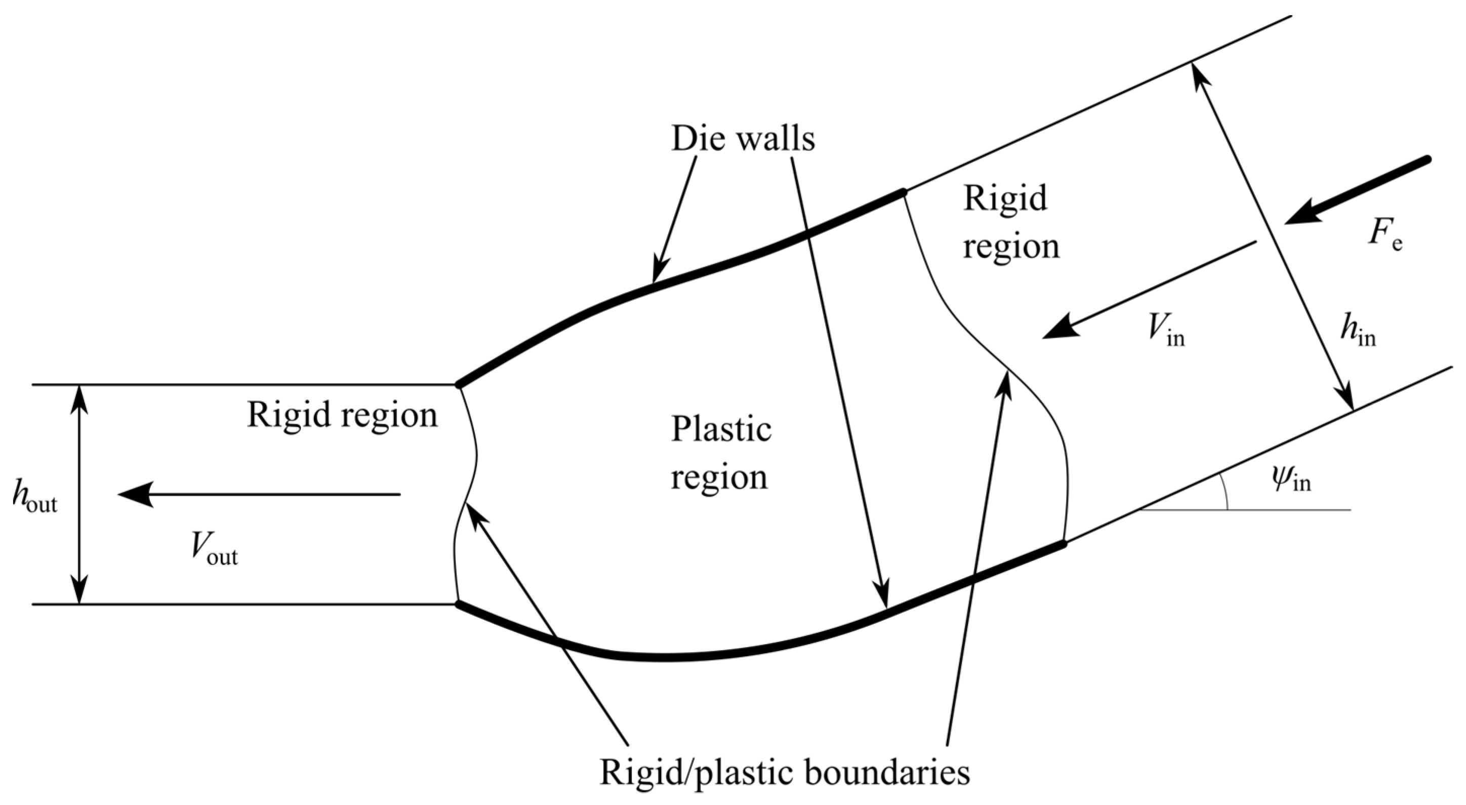
2. Statement of the Problem

A sheet of initial thickness hin is extruded through a frictionless die. The final thickness of the sheet is hout. The process is stationary, and the deformation is plane strain. The elastic portion of the strain tensor is neglected. A plastic region in the die connects two rigid regions. One of the rigid regions moves horizontally with velocity Vout after exiting the plastic region. The other rigid region approaches the plastic region with velocity Vin at some angle ψin measured from the horizontal direction. A schematic diagram of the extrusion process is shown in Figure 1, where Fe is the extrusion force. The die shape that produces the above processes under the ideal flow condition should be found in the course of the solution.
It is assumed that the material obeys the double shearing and rotation model [22]. The constitutive equations are the Mohr–Coulomb yield criterion and the plastic flow rule. Let σxx, σyy, and σxy be the stress components referred to Cartesian coordinates (x, y). The yield criterion is represented as
( σ x x + σ y y ) sin φ + ( σ x x σ y y ) 2 + 4 σ x y 2 = 2 k cos φ ,
where k is the cohesion, and φ is the angle of internal friction. It is convenient to represent the plastic flow rule in terms of the angle of inclination of the direction of the algebraically greater principal stress to the x-axis. This angle is denoted as ψ. Then, the plastic flow rule becomes
ξ x x + ξ y y = 0 , sin 2 ψ ( ξ x x ξ y y ) 2 cos 2 ψ ξ x y 2 sin φ ( ω x y + Ω ) = 0 .
Here, ξ x x , ξ y y , and ξ x y are the strain rate components in the Cartesian coordinates; ω x y is the only non-zero spin component in the Cartesian coordinates; and Ω is the intrinsic spin. In many cases, Ω = 0 [22,28]. The present paper is concerned with this version of the model. Then, Equation (2) becomes
ξ x x + ξ y y = 0 , sin 2 ψ ( ξ x x ξ y y ) 2 cos 2 ψ ξ x y 2 sin φ ω x y = 0 .
The constitutive equations above are supplemented with the stress equilibrium equations:
σ x x x + σ x y y = 0   and   σ x y x + σ y y y = 0 .
The ideal flow condition is that the trajectories of one of the principal stresses coincide with the streamlines. This condition and the equations above constitute an overdetermined system of equations. However, it has been shown in [23] that this system is compatible.

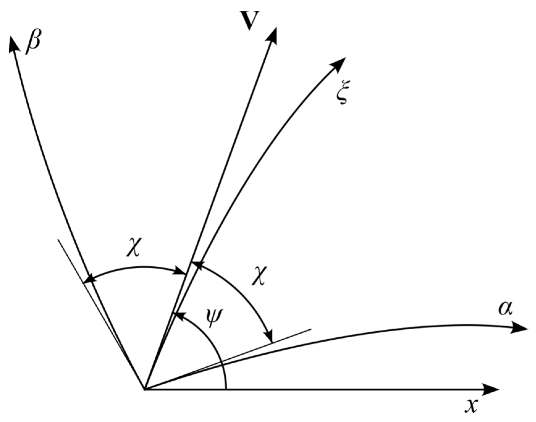
3. System of Equations in Characteristic Coordinates

Equations (1), (3), and (4) constitute a hyperbolic system. This section briefly summarizes available results concerning this system that are necessary for the subsequent solution.
Using a principal line coordinate system (ξ, η) for finding ideal flow solutions is convenient. The ξ-coordinate lines are the trajectories of the principal stress σξ, and the η-coordinate lines are the trajectories of the principal stress ση. It is assumed without loss of generality that
σ ξ > σ η .
Then, ψ involved in (3) is the anticlockwise angular rotation of the ξ-lines from the x-axis. The characteristic directions are determined as
H η H ξ d η d ξ = tan χ   and   H η H ξ d η d ξ = tan χ ,
where Hξ and Hη are the scale factors of the ξ- and η-coordinate curves, respectively, and χ = π / 4 + φ / 2 . The characteristic coordinates are denoted as (α, β). The first equation in (6) corresponds to the α-lines and the second to the β-lines. The ideal flow condition requires that the velocity vector V is tangent to the ξ-coordinate lines (Figure 2). The velocity vector may also be tangent to the η-coordinate lines. However, this condition is not required for the problem solved in the next section. The characteristic relations resulting from the stress equations are
cos φ d p + 2 ( p sin φ + cos φ ) d ψ = 0 along an α line , cos φ d p 2 ( p sin φ + cos φ ) d ψ = 0 along a β line ,
where
p = σ ξ + σ η 2 k .
It has been shown in [29] that it is always possible to put
ψ = ( α + β ) cos φ
in regions where both characteristic families are curved. In this case, Equation (7) allows for p to be determined as
ln ( p sin φ + cos φ p 0 sin φ + cos φ ) = 2 ( β α ) sin φ ,
where p0 is constant. It has been shown in [23] that the plastic flow rule is compatible with the ideal flow condition and the stress solution above if
V V 0 = ( p sin φ + cos φ p 0 sin φ + cos φ ) t ,
where V is the magnitude of V, V0 is constant, and t = sin φ 1 2 sin φ .
In regions where the α-lines are straight, Equations (9) and (10) are replaced with
ψ = ( α 0 + β ) cos φ ,   and   ln ( p sin φ + cos φ p 0 sin φ + cos φ ) = 2 ( β α 0 ) sin φ ,
where α0 is constant. Equation (11) is valid.
In regions where the β-lines are straight, Equations (9) and (10) are replaced with
ψ = ( α + β 0 ) cos φ   and   ln ( p sin φ + cos φ p 0 sin φ + cos φ ) = 2 ( β 0 α ) sin φ ,
where β0 is constant. Equation (11) is valid.
If the characteristic lines of both families are straight in a region, its motion is a rigid body translation.
The above equations show that calculating ideal flows mainly requires a characteristic network. The remaining calculations are merely manipulations with elementary functions.

4. Characteristic Network and Ideal Die Shapes

The solution for symmetric dies [23] allows for the general structure of the characteristic network to be guessed (Figure 3).

4.1. Special Solutions near the Die’s Exit

It is convenient to start analyzing this network from the die’s exit. Since the rigid region exiting the die moves horizontally, straight lines AD and AD’ are inclined to the horizontal line at angles χ, as shown in Figure 3. It has been taken into account here that the direction of the principal stress σξ is horizontal at point A. The position of point A relative to points D and D’ can be chosen arbitrarily, giving one of the parameters that control the characteristic network. It is convenient to choose the origin of the Cartesian coordinate system at point A. The distance between the x-axis and the center line of the sheet after exiting the die may serve as the noted parameter. This parameter is denoted as â (Figure 3). It varies in the range h out 2 a ^ h out 2 . It follows from the geometry of Figure 3 that the lengths of lines AD and AD’ are
r A D = ( h out 2 a ^ ) 1 sin χ   and   r A D = ( h out 2 + a ^ ) 1 sin χ .
Using this equation, one can find the Cartesian coordinates of points D and D’ in the form
x D = ( h out 2 a ^ ) cot χ ,   y D = h out 2 a ^ ,   x D = ( h out 2 + a ^ ) cot χ ,   and   y D = ( h out 2 + a ^ ) .
The orientation of the principal stress σξ at point A demands that AD is an α-line and AD’ is a β-line. Therefore, all α-lines are straight lines through D in region AFD. Similarly, all β-lines are straight lines through D’ in region AFD’. It follows from (6) that the angle between the characteristic directions equals 2χ. Therefore, AF and AF’ are logarithmic spirals. In particular, AF can be represented as
r = r A D exp ( θ tan φ ) .
Here, (r, θ) is the polar coordinate system with the origin at D, and θ is measured from line AD anticlockwise. Both families of characteristics are straight in DFC, where DC is a portion of the die’s surface. Therefore, the magnitude of angles FDC and DCF is χ. The inclination of DC to the x-axis is γ. The magnitude of this angle should be found in the course of the solution. It follows from the geometry of Figure 3 that the magnitude of angle ADF is also γ. Therefore, the length of DF is determined from (16) as
r D F = r A D exp ( γ tan φ ) .
Using this equation, one can find the length of DC as
r D C = 2 r A D exp ( γ tan φ ) cos χ .
The Cartesian coordinates of point C are determined by employing (14), (15), and (18) in the form
x C = ( h o u t 2 a ^ ) cot χ [ exp ( γ tan φ ) cos γ 1 2 ] , y C = ( h o u t 2 a ^ ) [ exp ( γ tan φ ) cot χ sin γ + 1 2 ] .
Since the magnitude of angle ADF is γ, region ADF vanishes if γ = 0. Therefore, the solution under construction is valid if
γ 0 .
Similarly, AF’ can be represented as
r = r A D exp ( θ tan φ ) .
Here, (r, θ) is the polar coordinate system with the origin at D’, and θ is measured from line AD’ clockwise. Both families of characteristics are straight in DFC’, where DC’ is a portion of the die’s surface. Therefore, the magnitude of angles FDC’ and DCF’ is χ. The inclination of DC’ to the x-axis is γ’. The magnitude of this angle should be found in the course of the solution. It follows from the geometry of Figure 3 that the magnitude of angle AD’F’ is also γ’. Therefore, the length of DF’ is determined from (21) as
r D F = r A D exp ( γ tan φ ) .
Using this equation, one can find the length of DC’ as
r D C = 2 r A D exp ( γ tan φ ) cos χ .
The Cartesian coordinates of point C’ are determined by employing (14), (15), and (23) in the form
x C = ( h o u t + 2 a ^ ) cot χ [ exp ( γ tan φ ) cos γ 1 2 ] , y C = ( h o u t + 2 a ^ ) [ exp ( γ tan φ ) cot χ sin γ + 1 2 ] .
Since the magnitude of angle ADF’ is γ’, region ADF’ vanishes if γ’ = 0. Therefore, the solution under construction is valid if
γ 0 .

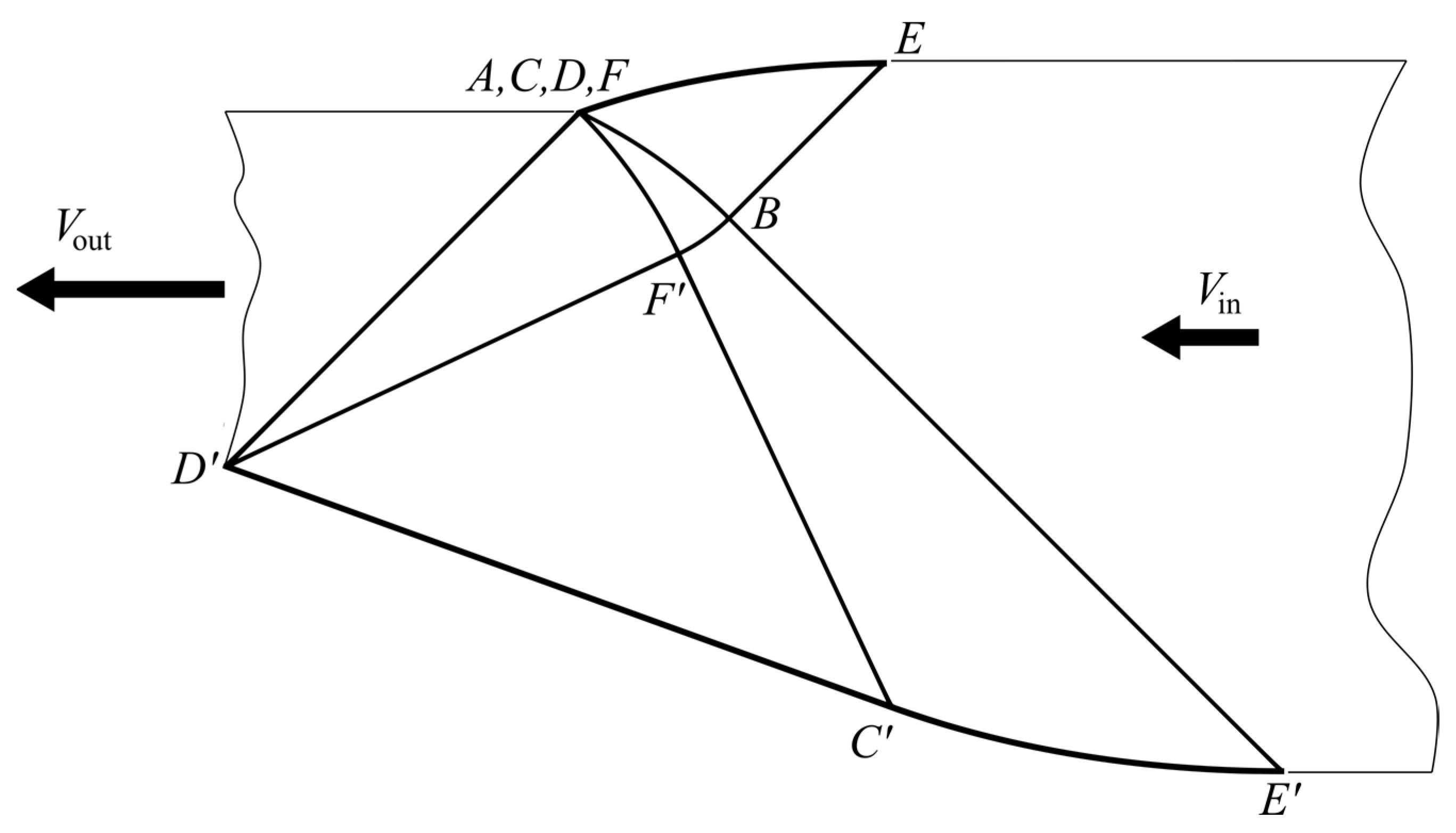
4.2. Region AFBF’ (Figure 3)

The characteristics of both families are curved in this region. Since ψ = 0 at point A, Equation (9) demands that the base α-line coincides with AF’ and the base β-line with AF (i.e., α = 0 on line AF, and β = 0 on line AF’). It follows from the geometry of Figure 3 that ψ = γ at point F and ψ = γ’ at point F’. Therefore, Equation (9) supplies the characteristic coordinates of points F’ and F in the form
α F = γ cos φ   and   β F = γ cos φ .
The radii of curvature of the α- and β-characteristic lines are denoted as R and S, respectively. These quantities can be defined as
1 R = ψ s α   and   1 S = ψ s β ,
where s α and s β denote differentiation along the α- and β-characteristic lines, respectively. It is advantageous to introduce the following quantities:
R 0 = R exp [ ( β α ) sin φ ]   and   S 0 = S exp [ ( β α ) sin φ ] .
It has been shown in [29] that these quantities satisfy the equations:
R 0 β = S 0   and   S 0 α = R 0 .
One can transform these equations to
2 R 0 α β + R 0 = 0   and   2 S 0 α β + S 0 = 0 .
Each of these equations is the equation of telegraphy. Therefore, they can be integrated by the method of Riemann. In particular, the Green’s function is
G ( a ,   b ,   α ,   β ) = J 0 [ 2 ( a α ) ( b β ) ] ,
where J 0 ( z ) is the Bessel function of zero order.
Formulating the boundary conditions on lines AF and AF’ requires calculating the radii of curvature of these lines. Differential geometry supplies the formula for the radius of curvature of a curve represented in polar coordinates. Substituting (16) and (21) into this formula and using (14), one arrives at
S A F = ( h out 2 a ^ ) 2 sin χ cos φ exp ( θ tan φ )   and   R A F = ( h out + 2 a ^ ) 2 sin χ cos φ exp ( θ tan φ ) ,
where SAF is the value of S on line AF, and RAF’ is the value of R on line AF’. Since ψ = 0, and θ = 0 at point A, Equations (9) and (32) combine to give
S A F ( β ) = ( h o u t 2 a ^ ) 2 sin χ cos φ exp ( β sin φ )   and   R A F ( α ) = ( h o u t + 2 a ^ ) 2 sin χ cos φ exp ( α sin φ ) .
Substituting SAF(β) into the second equation in (28) at α = 0 and RAF’(α) into the first equation in (28) at β = 0 supplies
S 0 A F = ( h o u t 2 a ^ ) 2 sin χ cos φ   and   R 0 A F = ( h o u t + 2 a ^ ) 2 sin χ cos φ ,
where S 0 A F is the value of S0 on line AF, and R 0 A F is the value R0 on line AF’. The equations in (34) are the boundary conditions for the equations in (30).
According to Riemann’s method, the value of S0 at a generic point P in region AFBF’ is determined from the following equation (Figure 4):
P P α ( S 0 G β G S 0 β ) d β + P α A ( G S 0 α S 0 G α ) d α +       + A P β ( S 0 G β G S 0 β ) d β + P β P ( G S 0 α S 0 G α ) d α = 0 .
These integrals are evaluated separately below. The value of S0 at point P is denoted as S 0 P .
It follows from (31) that G = 1 on lines PβP and PPα. Therefore,
P P α ( S 0 G β G S 0 β ) d β = S 0 A F + S 0 P   and   P β P ( G S 0 α S 0 G α ) d α = S 0 P S 0 A F ,
where S 0 A F is the value of S0 on line AF’. Employing (34), one can integrate the second equation in (29) to get
S 0 A F = R 0 A F α + S 0 A F .
Since S 0 = S 0 A F on APβ and G = 1 at point Pβ,
A P β ( S 0 G β G S 0 β ) d β = S 0 A F [ 1 J 0 ( 2 a b ) ] .
Here, Equation (31) has been used. Integrating by parts, one can transform the second integral in (35) as
P α A ( G S 0 α S 0 G α ) d α = a 0 ( G S 0 α S 0 G α ) d α = = a 0 [ 2 G S 0 α ( S 0 G ) α ] d α = 2 a 0 G S 0 α d α ( S 0 G ) | α = 0 + ( S 0 G ) | α = a .
Since S 0 = S 0 A F on APα, substituting (30) and (36) into (38) leads to
P α A ( G S 0 α S 0 G α ) d α = S 0 A F [ 1 J 0 ( 2 a b ) ] 2 R 0 A F a 0 J 0 [ 2 ( a α ) b ] d α .
This result can be further simplified taking into account that
d [ z J 1 ( z ) ] / d z = z J 0 ( z ) ,
where J 1 ( z ) is the Bessel function of first order. Put z = 2 ( a α ) b . Then, using (41), one gets
J 0 [ 2 ( a α ) b ] = d { ( a α ) b J 1 [ 2 ( a α ) b ] } b d α .
Substituting (42) into (40) yields
P α A ( G S 0 α S 0 G α ) d α = S 0 A F [ 1 J 0 ( 2 a b ) ] + 2 a b R 0 A F b J 1 ( 2 a b ) .
Equations (35), (36), (38), and (43) combine to give
S 0 P = S 0 A F J 0 ( 2 a b ) a b R 0 A F b J 1 ( 2 a b ) .
One can eliminate S 0 A F and R 0 A F in this equation employing (34). It is seen from (26) that ab < 0. Therefore, it is convenient to rewrite (44) as
S 0 P = S 0 A F I 0 ( 2 | a b | ) + | a b | R 0 A F I 1 ( 2 | a b | ) .
Here, I 0 ( z ) and I 1 ( z ) are the modified Bessel functions of zero and first orders, respectively.
Using the same line of reasoning as above, one can represent the solution of the first equation in (30) as
R 0 P = R 0 A F I 0 ( 2 | a b | ) + S 0 A F | b a | I 1 ( 2 | a b | ) .
The radius of curvature of line FB is determined from (28) and (46) as
R F B ( α ) = [ R 0 A F I 0 ( 2 | α b F | ) + S 0 A F | b F α | I 1 ( 2 | α b F | ) ] exp [ ( α β F ) sin φ ] .
Therefore, the Cartesian coordinates of this line can be represented by the equations
x F B = x F + cos φ 0 α [ R 0 A F I 0 ( 2 | a b F | ) + S 0 A F | b F a | I 1 ( 2 | a b F | ) ] exp [ ( a β F ) sin φ ] cos ( ψ χ ) d a , y F B = y F + cos φ 0 α [ R 0 A F I 0 ( 2 | a b F | ) + S 0 A F | b F a | I 1 ( 2 | a b F | ) ] exp [ ( a β F ) sin φ ] sin ( ψ χ ) d a .
Here ψ is determined from (9) as ψ = (a + βF) cos φ and α F a 0 . The x- and y- coordinates of point F are readily found from (14) and (17) as
x F = r D F cos ( χ γ ) r A D cos χ = ( h out 2 a ^ ) [ cos ( χ γ ) sin χ exp ( γ tan φ ) cot χ ] , y F = h out 2 r D F sin ( χ γ ) = ( h out 2 a ^ ) [ 1 exp ( γ tan φ ) sin ( χ γ ) sin χ ] .
The radius of curvature of line FB is determined from (28) and (45) as
S F B ( β ) = [ S 0 A F I 0 ( 2 | a F β | ) + | a F β | R 0 A F I 1 ( 2 | a F β | ) ] exp [ ( α F β ) sin φ ] .
Therefore, the Cartesian coordinates of this line can be represented by the equations
x F B = x F cos φ 0 β [ S 0 A F I 0 ( 2 | a F b | ) + | a F b | R 0 A F I 1 ( 2 | a F b | ) ] exp [ ( α F b ) sin φ ] cos ( ψ + χ ) d b , y F B = y F cos φ 0 β [ S 0 A F I 0 ( 2 | a F b | ) + | a F b | R 0 A F I 1 ( 2 | a F b | ) ] exp [ ( α F b ) sin φ ] sin ( ψ + χ ) d b .
Here ψ is determined from (9) as ψ = (αF’ + b) cos φ and 0 b β F . The x- and y- coordinates of point F’ are readily found from (14) and (22) as
x F = r D F cos ( χ γ ) r A D cos χ = ( h out 2 + a ^ ) [ cos ( χ γ ) sin χ exp ( γ tan φ ) cot χ ] , y F = h out 2 r D F sin ( χ γ ) = ( h out 2 + a ^ ) [ 1 exp ( γ tan φ ) sin ( χ γ ) sin χ ] .
The Cartesian coordinates of point B, xB and yB, are determined from (48) at a = αF’ or (51) at b = βF.

4.3. Regions FCEB and F’C’E’B (Figure 3)

The β-lines are straight in region FCEB. Therefore, the angle ψ is independent of β. Since ψ = γ and α = 0 on line CF, the dependence of this angle on α follows from (9) in the form
ψ = α cos φ + γ .
It follows from the geometry of Figure 3 that
x α = R cos φ cos ( ψ π 4 φ 2 ) , x β = T ( α ) sin ( ψ π 4 + φ 2 ) , y α = R cos φ sin ( ψ π 4 φ 2 ) , y β = T ( α ) cos ( ψ π 4 + φ 2 ) .
Here T(α) is an arbitrary function of α. The compatibility equations are
2 x α β = 2 x β α   and   2 y α β = 2 y β α .
Substituting (53) and (54) into (55) yields
R β cos φ cos ( ψ χ ) = d T d α cos ( ψ + χ ) T sin ( ψ + χ ) cos φ , R β cos φ sin ( ψ χ ) = d T d α sin ( ψ + χ ) + T cos ( ψ + χ ) cos φ .
One can solve these equations for the derivatives d T / d α and R / β . As a result,
d T d α = T sin φ   and   R β = T cos φ .
The solution of the first equation satisfying the condition T = 1 for α = 0 is
T = e α sin φ .
Substituting this solution in the second equation in (57) and integrating the resulting equation leads to
R = e α sin φ cos φ ( β β F ) + R F B ( α ) .
Here, the last term can be eliminated by employing (45), giving the dependence of R on α and β in region FCEB.
Curve CE bisects the angle between the α- and β- directions. Therefore, the equation for this curve is
d s α = d s β .
It follows from (56) that dsα = R cos φ dα, and dsβ = Tdβ. These Equations (58), (59), and (60) combine to give
d β d α = cos φ R F B ( α ) e α sin φ β + β F .
The solution of this equation satisfying the boundary condition β = βC for α = 0 is
β = β F + ( β C β F ) e α + e α cos φ 0 α R F B ( μ ) e μ ( 1 sin φ ) d μ .
Using (59) and (60), one can derive the following equations for determining curve CE:
d x d α = 2 cos χ cos ψ [ R F B ( α ) cos φ e α sin φ ( β β F ) ] , d y d α = 2 cos χ sin ψ [ R F B ( α ) cos φ e α sin φ ( β β F ) ] .
In these equations, β should be eliminated by means of (62) and ψ by means of (53). Integrating the resulting equations gives
x C E = 2 cos χ 0 α cos ψ [ R F B ( η ) cos φ e η sin φ ( β β F ) ] d η + x C , y C E = 2 cos χ 0 α sin ψ [ R F B ( η ) cos φ e η sin φ ( β β F ) ] d η + y C .
Here 0 α α F . Equation (19) provides the values of xC and yC. Integrating by parts in (64) simplifies subsequent numerical integration. As a result,
x C E ( α ) = 2 cos χ cos φ 0 α R F B ( μ ) cos ( μ cos φ + γ ) d μ     ( β C β F ) cos χ ( 1 sin φ ) { v 1 ( α ) e α ( 1 sin φ ) + cos γ sin ( φ + γ ) }     cos χ cos φ ( 1 sin φ ) { v 1 ( α ) e α ( 1 sin φ ) 0 α R F B ( μ ) e μ ( 1 sin φ ) d μ 0 α R F B ( μ ) v 1 ( μ ) d μ } + x C , y C E ( β ) = 2 cos χ cos φ 0 α R F B ( μ ) sin ( μ cos φ + γ ) d μ + + ( β C β F ) cos χ ( 1 sin φ ) [ v 2 ( α ) e α ( 1 sin φ ) sin γ cos ( φ + γ ) ] +     + cos χ cos φ ( 1 sin φ ) { v 2 ( α ) e α ( 1 sin φ ) 0 α R F B ( μ ) e μ ( 1 sin φ ) d μ 0 α R F B ( μ ) v 2 ( μ ) d μ } + y C ,
where
v 1 ( z ) = sin ( z cos φ + γ + φ ) cos ( z cos φ + γ ) , v 2 ( z ) = sin ( z cos φ + γ ) + cos ( z cos φ + γ + φ ) .
This solution supplies the shape of wall CE in parametric form. In particular, the Cartesian coordinates of point E are determined from (65) as
x E = x C E ( α F )   and   y E = y C E ( α F ) .
Region FCEB, where the α-lines are straight, can be treated similarly. The angle ψ is independent of α. Since ψ = −γ’ and α = 0 on line CF’, the dependence of this angle on β follows from (9) in the form
ψ = β cos φ γ .
It follows from the geometry of Figure 3 that
x α = T 2 ( β ) cos ( ψ π 4 φ 2 ) , x β = S cos φ sin ( ψ π 4 + φ 2 ) , y α = T 2 ( β ) sin ( ψ π 4 φ 2 ) , y β = S cos φ cos ( ψ π 4 + φ 2 ) .
Here, T2(β) is an arbitrary function of β. Substituting (68) and (69) into (55) yields
S α cos φ cos ( ψ + χ ) = d T 2 d β cos ( ψ χ ) + T 2 sin ( ψ χ ) cos φ , S α cos φ sin ( ψ + χ ) = d T 2 d β sin ( ψ χ ) T 2 cos ( ψ χ ) cos φ .
One can solve these equations for the derivatives d T 2 d β and S α . As a result,
d T 2 d β = T 2 sin φ ,   and   S α = T 2 cos φ .
The solution of the first equation satisfying the condition T2 = 1 for β = 0 is
T 2 = e β sin φ .
Substituting this solution in the second equation in (71) and integrating the resulting equation leads to
S = exp ( β sin φ ) cos φ ( α α F ) + S F B ( β ) .
Here, the last term can be eliminated by employing (50), giving the dependence of S on α and β in region FCEB.
Curve CE’ bisects the angle between the α- and β- directions. Therefore, Equation (60) is valid. It follows from (70) that d s β = S cos φ d β , and d s α = T 2 d α . These Equations, (60), (72), and (73) combine to give
d α d β = cos φ S F B ( β ) e β sin φ + α α F .
The solution of this equation satisfying the boundary condition α = αC’ for β = 0 is
α = α F + ( α C α F ) e β e β cos φ 0 β S F B ( μ ) e μ ( 1 sin φ ) d μ .
Using (60) and (73), one can derive the equations for determining curve CE’ in the form
d x d β = 2 cos χ cos ψ [ S F B ( β ) cos φ e β sin φ ( α α F ) ] , d y d β = 2 cos χ sin ψ [ S F B ( β ) cos φ e β sin φ ( α α F ) ] .
In these equations, α should be eliminated by means of (75) and ψ by means of (68). Integrating the resulting equations gives
x C E ( β ) = 2 cos χ 0 β cos ψ [ S F B ( μ ) cos φ exp μ sin φ ( α α F ) ] d μ + x C , y C E ( β ) = 2 cos χ 0 β sin ψ [ S F B ( μ ) cos φ exp μ sin φ ( α α F ) ] d μ + y C .
Here 0 β β F . Equation (19) provides the values of xC’ and yC’. Integrating by parts in (77) simplifies subsequent numerical integration. As a result,
x C E ( β ) = 2 cos χ cos φ 0 β S F B ( μ ) cos ( μ cos φ γ ) d μ +     + ( α C α F ) cos χ ( 1 sin φ ) { u 1 ( β ) e β ( 1 sin φ ) cos γ + sin ( φ + γ ) }     cos χ cos φ ( 1 sin φ ) { u 1 ( β ) e β ( 1 sin φ ) 0 β S F B ( μ ) e μ ( 1 sin φ ) d μ 0 β S F B ( μ ) u 1 ( μ ) d μ } , y C E ( β ) = 2 cos χ cos φ 0 β S F B ( μ ) sin ( μ cos φ γ ) d μ +    + ( α C α F ) cos χ ( 1 sin φ ) [ u 2 ( β ) e β ( 1 sin φ ) + sin γ + cos ( φ + γ ) ]     cos χ cos φ ( 1 sin φ ) { u 2 ( β ) e β ( 1 sin φ ) 0 β S F B ( μ ) e μ ( 1 sin φ ) d μ 0 β S F B ( μ ) u 2 ( μ ) d μ } ,
where
u 1 ( z ) = cos ( z cos φ γ ) + sin ( z cos φ γ φ ) , u 2 ( z ) = sin ( z cos φ γ ) cos ( z cos φ γ φ ) .
Equation (78) supplies the shape of wall CE’ in parametric form. In particular, the Cartesian coordinates of point E’ are determined from (78) as
x E = x C E ( β F )   and   y E = y C E ( β F ) .

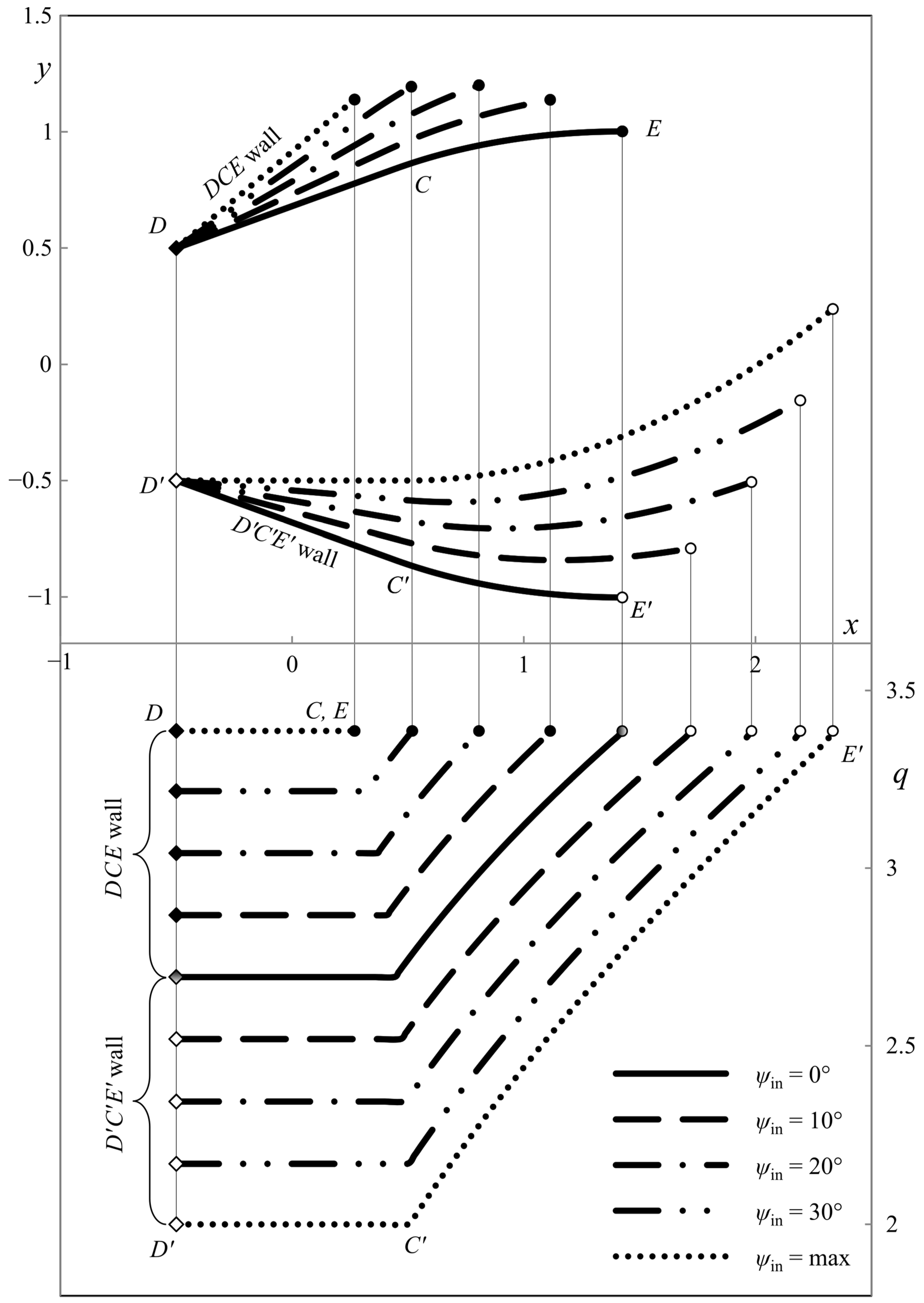
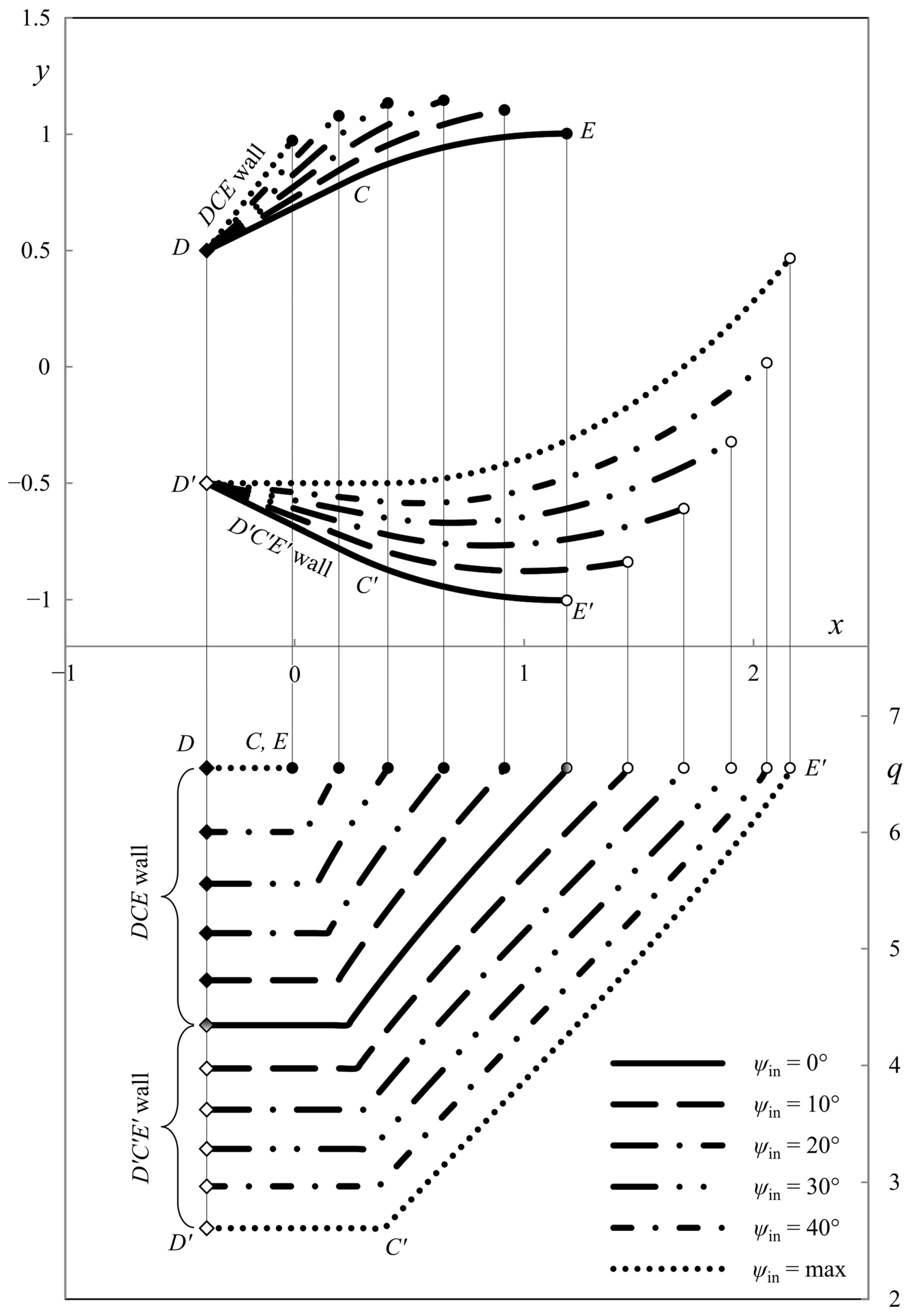
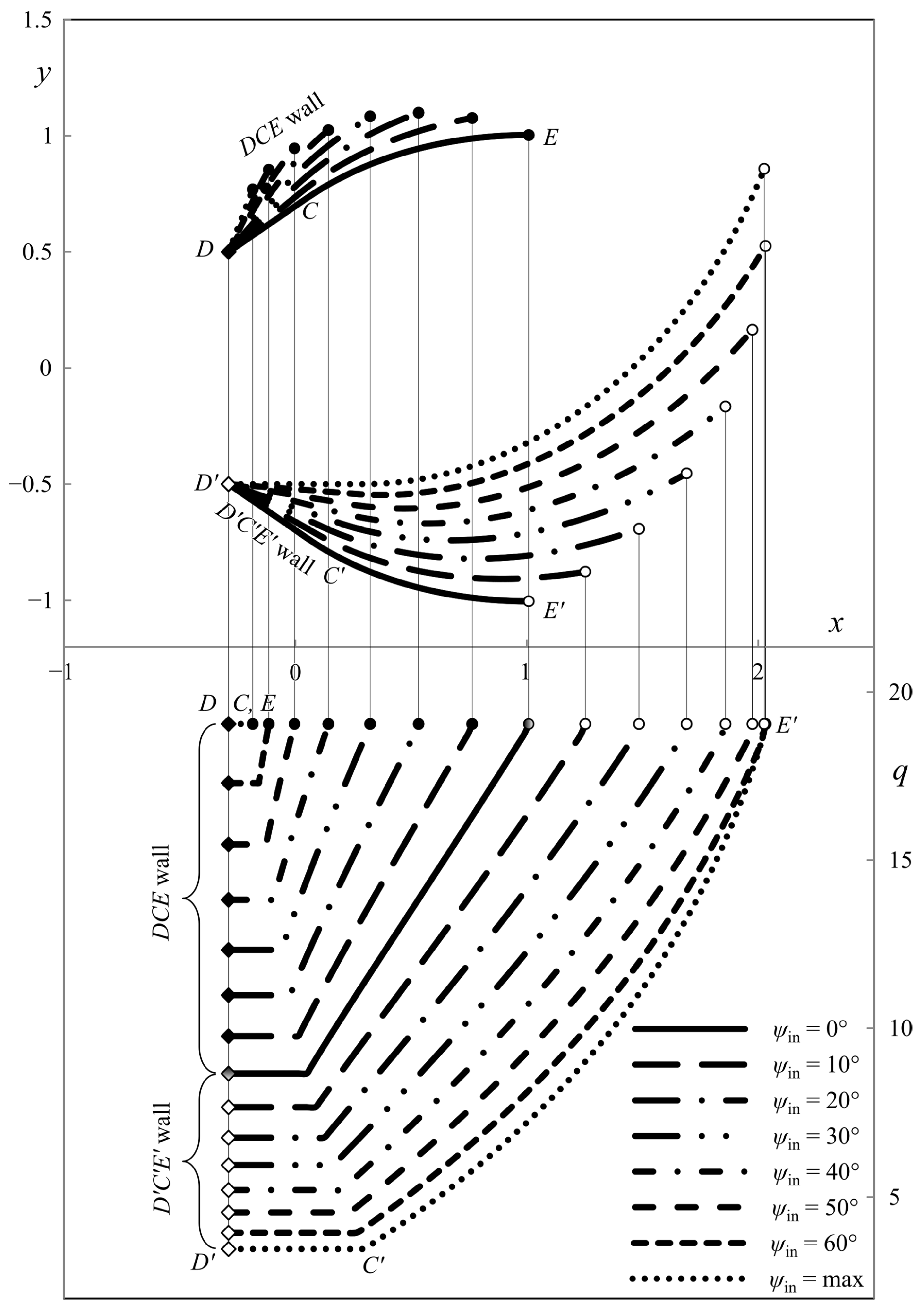
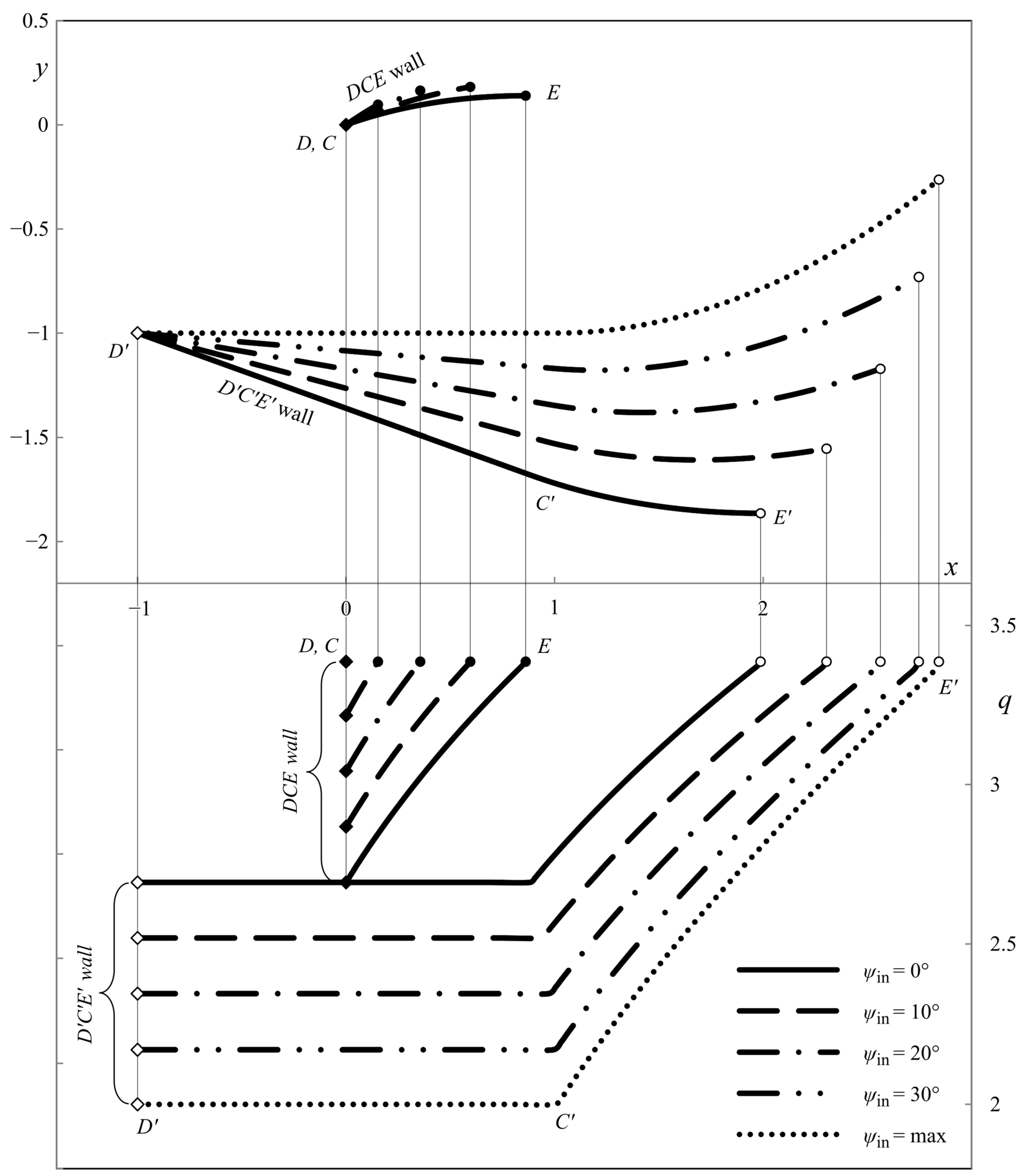
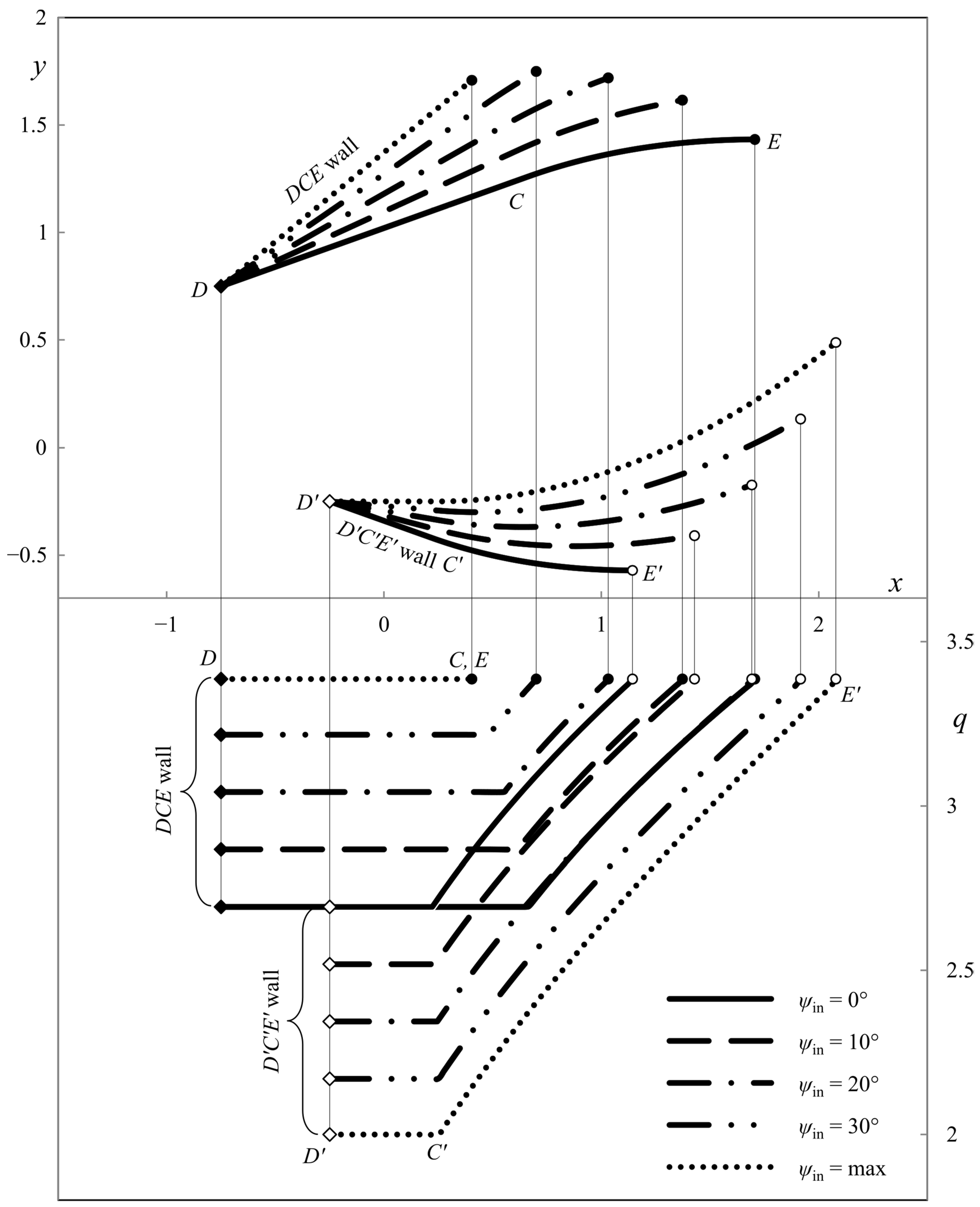
4.4. Ideal Die Shapes

The general solution in Section 4.1, Section 4.2 and Section 4.3 determines the shapes of DCE and D’C’E’ (Figure 3) and contains three parameters: γ, γ’, and â. The process is classified by two independent parameters, hin/hout and ψin (Figure 1). To calculate an ideal die for a specific process, one must connect the first group of the parameters and the second.
It is seen from Figure 3 that ψ = ψin at point B. On the other hand, α = αF’, and β = β F, at this point. Therefore, it follows from (9) and (26) that
ψ in = γ γ
In particular, ψin = 0, and γ = γ’, in the case of symmetric dies.
It follows from (10) and (11) that
ln V V 0 = ( 1 sin φ ) ( α β ) .
Since α = 0 and β = 0 at point A, it follows from (82) that V0 = Vout, and
ln V in V out = ( 1 sin φ ) ( α F β F ) .
The material is incompressible. Therefore, Vouthout = Vinhin. This equation, (26), and (83) combine to give
ln h in h out = ( γ + γ ) cot χ .
Solving Equations (81) and (84) for γ and γ’ supplies
γ = 1 2 [ ln ( h in h out ) tan χ + ψ in ]   are   γ = 1 2 [ ln ( h in h out ) tan χ ψ in ] .
Since hin/hout > 1 and ψin ≥ 0, the first equation in (85) shows that the inequality in (20) is automatically satisfied. The second equation in (85) and the inequality in (25) impose the following restriction on the process parameters:
ln ( h in / h out ) tan χ ψ in .
The parameter â is not connected to hin/hout and ψin. It can be used for calculating different ideal dies for the same process (i.e., for the same values of hin/hout and ψin). This parameter may vary in the range
h out / 2 a ^ h out / 2 .

4.5. Special Solutions

Some regions shown in Figure 3 degenerate to lines or points at certain values of the parameters classifying the characteristic network. One of the special solutions is obtained if γ’ = 0. In this case, angle ADF’ vanishes, and line DAFC’ becomes straight. This straight line is the rigid/plastic boundary, and triangle DFC’ becomes a part of the rigid sheet that exits the die. Since line AF’ degenerates to a point, region DAFCEBF becomes a characteristic fan with a point singularity D. Thus, line DFBE’ becomes straight, and region DFBEC becomes a triangle, which can be treated as a part of the rigid sheet that enters the die. Therefore, line DFBE’ is the rigid/plastic boundary. Figure 5 illustrates the characteristic network. It is seen from (85) that this special solution corresponds to the maximum possible value of ψin at a given ratio hin/hout. This maximum value is readily determined from (86). It is clear from the above that the value of â is immaterial for this special solution.
Another special solution is obtained if â = hout/2. Line AD and region AFCD degenerate to points. The solution given in Section 4.2 is not required for calculating the characteristic network. The value of â is immaterial for this special solution. Any value of ψin that satisfies (86) can be chosen. Figure 6 illustrates the characteristic network at ψin = 0.

5. Pressure on the Die’s Walls

The pressure on the die’s walls is important for the process design. In particular, it is involved in many empirical equations for calculating the wear of tools [30,31,32,33]. Since the die is frictionless, the normal stress acting on the die’s walls equals ση. The principal stresses are readily found by employing the solution in Section 4.
In terms of the principal stresses, Equation (1) has the following form:
p sin φ + σ ξ σ η 2 k = cos φ .
Using (8) and (88), one can represent the principal stresses as
σ ξ / k = cos φ ( 1 sin φ ) p   and   σ η / k = cos φ ( 1 + sin φ ) p .
Since σξ = 0 on lines AD and AD’, it follows from (10) and the first equation in (89) that
p 0 = tan χ .
Equations (12) and (90) supply the value of p in region DFC, where the principal stresses are constant. In particular,
p D F C = ( tan χ + cot φ ) exp ( 2 γ tan φ ) cot φ .
Then, the dimensionless pressure on the die’s wall between points D and C is determined from (89) and (91) as
q = | σ η | / k = | cos φ ( 1 + sin φ ) [ ( tan χ + cot φ ) exp ( 2 γ tan φ ) cot φ ] | .
Similarly, the dimensionless pressure on the die’s wall between points D’ and C’ is determined as
q = | σ η | / k = | cos φ ( 1 + sin φ ) [ ( tan χ + cot φ ) exp ( 2 γ tan φ ) cot φ ] | .
Note that
lim φ 0 q = 2 + 2 γ   and   lim φ 0 q = 2 + 2 γ
on walls DC and DC’, respectively.
Equation (13) is valid in region CFBE. Therefore, taking into account (90), one can get
p = ( tan χ + cot φ ) exp [ 2 ( γ tan φ α sin φ ) ] cot φ .
The second equation in (89) and (95) combine to give
q = | cos φ ( 1 + sin φ ) { ( tan χ + cot φ ) exp [ 2 ( γ tan φ α sin φ ) ] cot φ } | .
This equation provides the pressure on the die between points C and E. Equations (65) and (96) allow the pressure distribution to be calculated in the Cartesian coordinates.
One can similarly derive the equation for the pressure on the die between points C’ and E’. As a result,
q = | cos φ ( 1 + sin φ ) { ( tan χ + cot φ ) exp [ 2 ( γ tan φ + β sin φ ) ] cot φ } | .
This equation and (78) allow the pressure distribution to be calculated in the Cartesian coordinates.
It follows from (7) that p is constant along lines EB and E’B. Therefore, it is constant along the entire rigid/plastic boundary. Thus, the value of p is the same at points E and E’. Then, it follows from (89) that the value of q is the same at these points. This value can be found from (96) or (97) using (26). As a result,
q E , E = | cos φ ( 1 + sin φ ) { ( tan χ + cot φ ) exp [ 2 ( γ + γ ) tan φ ] cot φ } | .
Eliminating in this equation γ and γ’ employing (84), one gets
q E , E = | cos φ ( 1 + sin φ ) { ( tan χ + cot φ ) ( h in / h out ) 2 tan φ tan χ cot φ } | .
It follows from this equation that
lim φ 0 q E , E = 2 + 2 ( γ + γ ) = 2 + 2 ln ( h in / h out )
Equation (99) shows that the value of q at points E and E’ is independent of ψin.
Since the value of q on the rigid/plastic boundary has been found, the principal stress σ ξ is readily determined from (89) by eliminating p. The quantity σ ξ / k may be regarded as a dimensionless extrusion force.

6. Illustrative Examples

This section presents the numerical results demonstrating the process parameters’ effect on the ideal die shape and wall pressure. The deviation from the symmetric shape is emphasized. All the calculations have been performed for hin/hout = 2. Figure 7, Figure 8 and Figure 9 show several die profiles and the corresponding wall pressure distributions at â =0. The parameter ψin varies from 0 (symmetric dies) to its maximum value determined by Equation (86). Different figures correspond to different values of the angle of internal friction. In particular, φ = 0 in Figure 7 (pressure-independent material); φ = 15° in Figure 8; and φ = 30° in Figure 9.
The influence of parameter â is revealed in Figure 10, Figure 11, Figure 12 and Figure 13. In these cases, φ = 0. As in Figure 7, Figure 8 and Figure 9 the parameter ψin varies from 0 to its maximum value. Also, â = hout/4 in Figure 10; â = hout/2 in Figure 11; â = −hout/4 in Figure 12; and â = −hout/2 in Figure 13. The dies in Figure 11 and Figure 13 correspond to the special solutions discussed in Section 4.5.
The numerical results show that the length of the upper wall decreases, and the length of the lower wall increases as parameter ψin increases. The leftmost point of the upper die is to the right of the leftmost point of the lower die if â > 0. Accordingly, the leftmost point of the upper die is to the left to the leftmost point of the lower die if â < 0. The pressure on the upper die is always higher than on the lower die, except for the symmetric dies.

7. Conclusions

A new general stationary planar ideal flow solution has been found for the double slip and rotation model. Its distinguishing feature, as compared to other planar ideal flow solutions, is that the flow has no symmetry axis. The solution in Section 4 includes all possible ideal flows, assuming that the characteristic field is singular at the die’s exit (Figure 3). Generally, the characteristic network consists of three types of regions. Both families of characteristics are straight in the regions of one type; the characteristics of one family are curved in the regions of the second type; and both families of characteristics are curved in the regions of the third type. However, some of these regions may not exist under certain conditions. The solution is purely analytical in the regions where the characteristics of at least one family are curved. Riemann’s method is employed for calculating the characteristic network in the regions where both families of characteristics are curved. In this case, a numerical technique is only necessary to evaluate ordinary integrals. It is known that Riemann’s method is very accurate, and corresponding solutions can be used to verify the accuracy of numerical solutions [34]. The general solution is used to show the effect of process and material parameters on the ideal die’s shape and the distribution of wall pressures. The corresponding symmetric shapes are obtained as a particular case. The die’s shapes calculated are compared to shapes for pressure-independent material.

Author Contributions

Formal analysis, V.M.; conceptualization, S.A.; supervision, S.A.; writing—original draft, S.A. and V.M. All authors have read and agreed to the published version of the manuscript.

Funding

The study was supported by the Russian State Assignment (contracts #123021700045-7, #123021700050-1).

Institutional Review Board Statement

Not applicable.

Informed Consent Statement

Not applicable.

Data Availability Statement

Data is contained within the article.

Acknowledgments

This publication has been supported by the RUDN University Scientific Projects Grant System, project No. 202247-2-000.

Conflicts of Interest

The authors declare no conflict of interest.

References

  1. Chung, K.; Alexandrov, S. Ideal Flow in Plasticity. Appl. Mech. Rev. 2007, 60, 316–335. [Google Scholar] [CrossRef]
  2. Richmond, O.; Devenpeck, M.L. A die profile for maximum efficiency in strip drawing. In Proceedings of the 4th U.S. National Congress of Applied Mechanics, Berkeley, CA, USA, 18–21 June 1962; pp. 1053–1057. [Google Scholar]
  3. Devenpeck, M.L.; Richmond, O. Strip-Drawing Experiments with a Sigmoidal Die Profile. J. Manuf. Sci. Eng. 1965, 87, 425–428. [Google Scholar] [CrossRef]
  4. Richmond, O.; Morrison, H.L. Streamlined wire drawing dies of minimum length. J. Mech. Phys. Solids 1967, 15, 195–203. [Google Scholar] [CrossRef]
  5. Hill, R. Ideal forming operations for perfectly plastic solids. J. Mech. Phys. Solids 1967, 15, 223–227. [Google Scholar] [CrossRef]
  6. Richmond, O.; Alexandrov, S. The theory of general and ideal plastic deformations of Tresca solids. Acta Mech. 2002, 158, 33–42. [Google Scholar] [CrossRef]
  7. Cox, A.D.; Eason, G.; Hopkins, H.G. Axially symmetric plastic deformations in soils. Philos. Trans. R. Soc. Lond. Ser. A Math. Phys. Sci. 1961, 254, 1–45. [Google Scholar] [CrossRef]
  8. Cox, G.M.; Thamwattana, N.; McCue, S.W.; Hill, J.M. Coulomb–Mohr Granular Materials: Quasi-static Flows and the Highly Frictional Limit. Appl. Mech. Rev. 2008, 61, 060802. [Google Scholar] [CrossRef]
  9. Coombs, W.M.; Crouch, R.S.; Heaney, C.E. Observations on Mohr-Coulomb Plasticity under Plane Strain. J. Eng. Mech. 2013, 139, 1218. [Google Scholar] [CrossRef]
  10. Lomakin, E.; Beliakova, T. Spherically symmetric deformation of solids with nonlinear stress-state-dependent properties. Contin. Mech. Thermodyn. 2023, 35, 1721–1733. [Google Scholar] [CrossRef]
  11. Mehrabadi, M.M.; Cowin, S.C. Initial planar deformation of dilatant granular materials. J. Mech. Phys. Solids 1978, 26, 269–284. [Google Scholar] [CrossRef]
  12. Kruyt, N.P. An analysis of the generalized double-sliding models for cohesionless granular materials. J. Mech. Phys. Solids 1990, 38, 27–35. [Google Scholar] [CrossRef]
  13. Spencer, A.J.M. A theory of the kinematics of ideal soils under plane strain conditions. J. Mech. Phys. Solids 1964, 12, 337–351. [Google Scholar] [CrossRef]
  14. Marshall, E.A. The compression of a slab of ideal soil between rough plates. Acta Mech. 1967, 3, 82–92. [Google Scholar] [CrossRef]
  15. Pemberton, C.S. Flow of imponderable granular materials in wedge-shaped channels. J. Mech. Phys. Solids 1965, 13, 351–360. [Google Scholar] [CrossRef]
  16. Spencer, A.J.M. Deformation of ideal granular materials. In Mechanics of Solids, The Rodney Hill 60th Anniversary Volume; Hopkins, H.G., Sewell, M.J., Eds.; Pergamon Press: Oxford, UK, 1982; pp. 607–652. [Google Scholar]
  17. Spitzig, W.A.; Sober, R.J.; Richmond, O. The effect of hydrostatic pressure on the deformation behavior of maraging and HY-80 steels and its implications for plasticity theory. Metall Trans A 1976, 7, 1703–1710. [Google Scholar] [CrossRef]
  18. Brownrigg, A.; Spitzig, W.A.; Richmond, O.; Teirlinck, D.; Embury, J.D. The influence of hydrostatic pressure on the flow stress and ductility of a spherodized 1045 steel. Acta Metallurg. 1983, 31, 1141–1150. [Google Scholar] [CrossRef]
  19. Spitzig, W.A.; Richmond, O. The effect of pressure on the flow stress of metals. Acta Metallurg. 1984, 32, 457–463. [Google Scholar] [CrossRef]
  20. Savage, J.C.; Lockner, D.A. A test of the double-shearing model of flow for granular materials. J. Geophys. Res. 1997, 102, 12287–12294. [Google Scholar] [CrossRef]
  21. Jiang, M.J.; Liu, J.D.; Arroyo, M. Numerical evaluation of three non-coaxial kinematic models using the distinct element method for elliptical granular materials. Int. J. Numer. Anal. Methods Geomech. 2016, 40, 2468–2488. [Google Scholar] [CrossRef]
  22. Harris, D. Double shearing and double rotation: A generalisation of the plastic potential model in the mechanics of granular materials. Int. J. Eng. Sci. 2009, 47, 1208–1215. [Google Scholar] [CrossRef]
  23. Alexandrov, S.; Mokryakov, V. Design of Dies of Minimum Length Using the Ideal Flow Theory for Pressure-Dependent Materials. Mathematics 2023, 11, 3726. [Google Scholar] [CrossRef]
  24. Hill, R. A remark on diagonal streaming in plane plastic strain. J. Mech. Phys. Solids 1966, 14, 245–248. [Google Scholar] [CrossRef]
  25. Alexandrov, S.; Pirumov, A. A Die Profile for Maximum Efficiency in Strip Drawing of Anisotropic Materials. Procedia Manuf. 2018, 21, 60–67. [Google Scholar] [CrossRef]
  26. Alexandrov, S.; Mokryakov, V.; Date, P. Ideal Flow Theory of Pressure-Dependent Materials for Design of Metal Forming Processes. Mater. Sci. Forum 2018, 920, 193–198. [Google Scholar] [CrossRef]
  27. Min, F.; Liu, H.; Zhu, G.; Chang, Z.; Guo, N.; Song, J. The streamlined design of self-bending extrusion die. Int. J. Adv. Manuf. Technol. 2021, 116, 363–373. [Google Scholar] [CrossRef]
  28. Harris, D. Some Properties of a New Model for Slow Flow of Granular Materials. Meccanica 2006, 41, 351–362. [Google Scholar] [CrossRef]
  29. Alexandrov, S. Geometry of plane strain characteristic fields in pressure-dependent plasticity. ZAMM-J. Appl. Math. Mech. Z. Angew. Math. Mech. 2015, 95, 1296–1301. [Google Scholar] [CrossRef]
  30. Lindqvist, M.; Evertsson, C.M. Development of wear model for cone crushers. Wear 2006, 261, 435–442. [Google Scholar] [CrossRef]
  31. Popov, V. Generalized Archard law of wear based on Rabinowicz criterion of wear particle formation. Mech. Eng. 2019, 17, 39–45. [Google Scholar] [CrossRef]
  32. Farzad, H.; Ebrahimi, R. An investigation of die profile effect on die wear of plane strain extrusion using incremental slab method and finite element analysis. Int. J. Adv. Manuf. Technol. 2020, 111, 627–644. [Google Scholar] [CrossRef]
  33. Bang, J.; Kim, M.; Bae, G.; Kim, H.-G.; Lee, M.-G.; Song, J. Efficient Wear Simulation Methodology for Predicting Nonlinear Wear Behavior of Tools in Sheet Metal Forming. Materials 2022, 15, 4509. [Google Scholar] [CrossRef] [PubMed]
  34. Hill, R.; Lee, E.H.; Tupper, S.J. A Method of Numerical Analysis of Plastic Flow in Plane Strain and Its Application to the Compression of a Ductile Material Between Rough Plates. J. Appl. Mech. 1951, 18, 46–52. [Google Scholar] [CrossRef]
Figure 1. Schematic diagram of the extrusion process.
Materials 16 07378 g001
Figure 2. Characteristic coordinates and the velocity vector.
Materials 16 07378 g002
Figure 3. General structure of the characteristic network.
Materials 16 07378 g003
Figure 4. Characteristic lines for Riemann’s method of integration (α = a on PPα, and β = b on PPβ).
Materials 16 07378 g004
Figure 5. General structure of the characteristic network corresponding to the special solution γ’ = 0.
Materials 16 07378 g005
Figure 6. General structure of the characteristic network corresponding to the special solution â = hout/2 at ψin = 0.
Materials 16 07378 g006
Figure 7. Die shape (upper diagram) and wall pressures (lower diagram) at φ = 0° and â = 0.
Materials 16 07378 g007
Figure 8. Die shape (upper diagram) and wall pressures (lower diagram) at φ = 15° and â = 0.
Materials 16 07378 g008
Figure 9. Die shape (upper diagram) and wall pressures (lower diagram) at φ = 30° and â = 0.
Materials 16 07378 g009
Figure 10. Die shape (upper diagram) and wall pressures (lower diagram) at φ = 0° and â = hout/4.
Materials 16 07378 g010
Figure 11. Die shape (upper diagram) and wall pressures (lower diagram) at φ = 0° and â = hout/2.
Materials 16 07378 g011
Figure 12. Die shape (upper diagram) and wall pressures (lower diagram) at φ = 0° and â = −hout/4.
Materials 16 07378 g012
Figure 13. Die shape (upper diagram) and wall pressures (lower diagram) at φ = 0° and â = −hout/2.
Materials 16 07378 g013
Disclaimer/Publisher’s Note: The statements, opinions and data contained in all publications are solely those of the individual author(s) and contributor(s) and not of MDPI and/or the editor(s). MDPI and/or the editor(s) disclaim responsibility for any injury to people or property resulting from any ideas, methods, instructions or products referred to in the content.

