


A Review on Friction Stir Welding/Processing: Numerical Modeling


Abstract
:1. Introduction
- Examining different numerical models for process simulation.
- Temperature, stress, and strain distributions during the process.
- Modeling the material flow in different types of FSW.
- Modeling the microstructural evolutions during the process.
2. Process Modeling Techniques
- 1.
- 2.
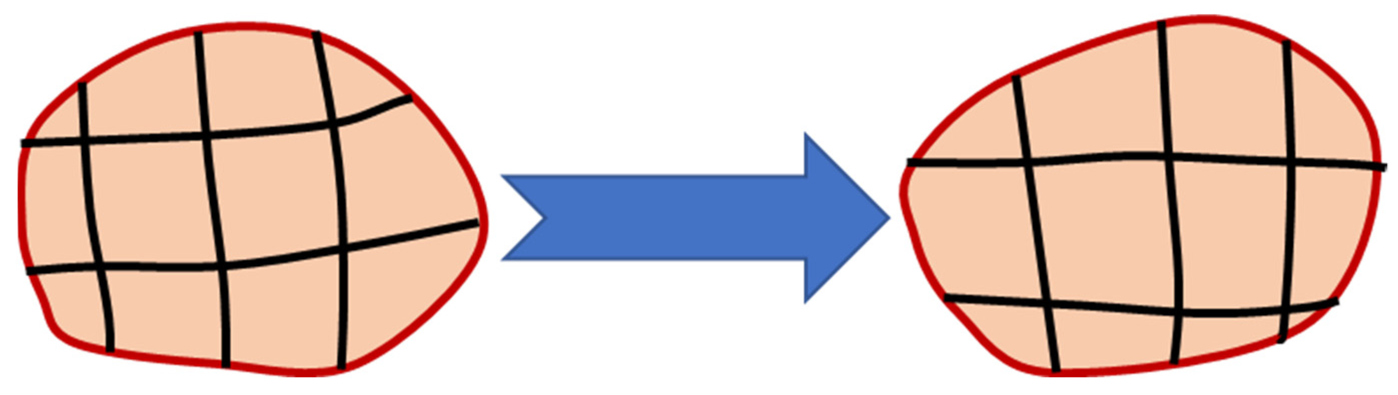
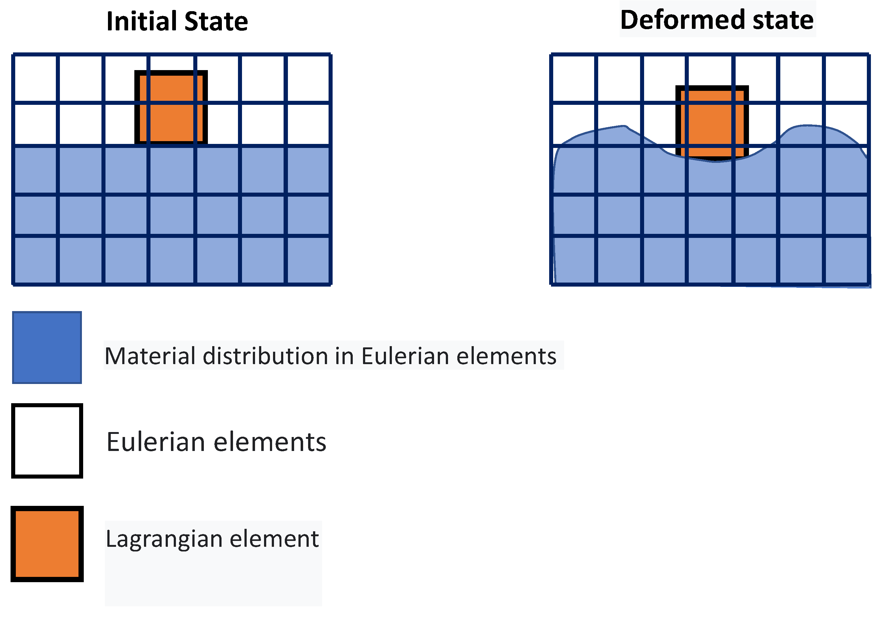
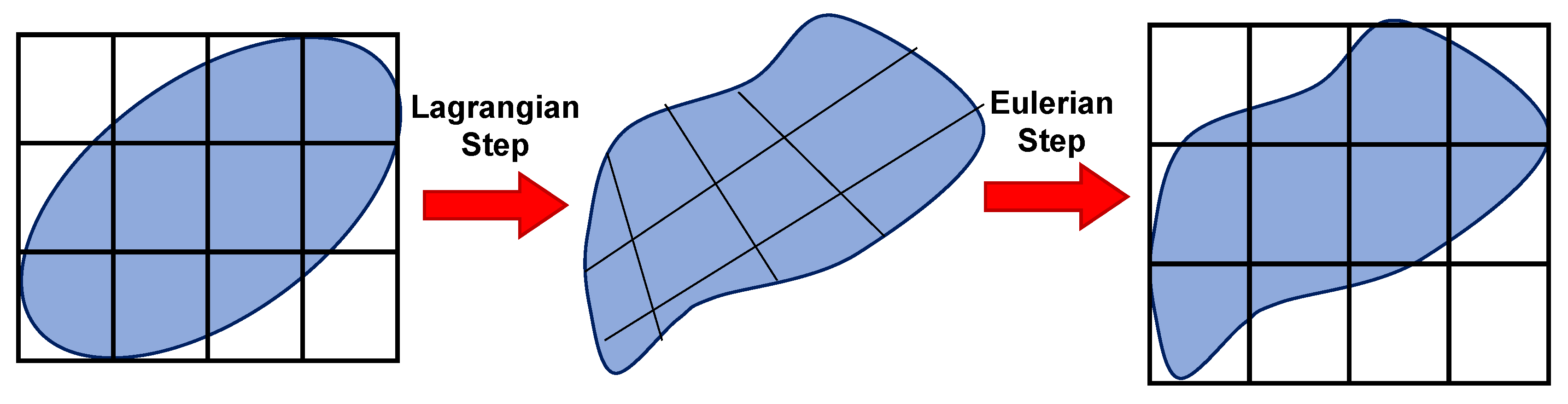
- Computational solid mechanics (CSM) models. Within CSM, two principal methods have been employed: the arbitrary Lagrangian–Eulerian (ALE) [49,50,51,52,53,54,55,56,57,58,59,60,61,62] method, the coupled Eulerian–Lagrangian (CEL) approach [63,64,65,66,67,68,69,70,71,72,73,74,75,76,77,78,79,80,81,82,83,84], and the smoothed particle hydrodynamics (SPH) method.
2.1. Computational Fluid Dynamics Models (CFD)
2.2. Numerical Models Based on Solid Mechanics (CMS)
- 1.
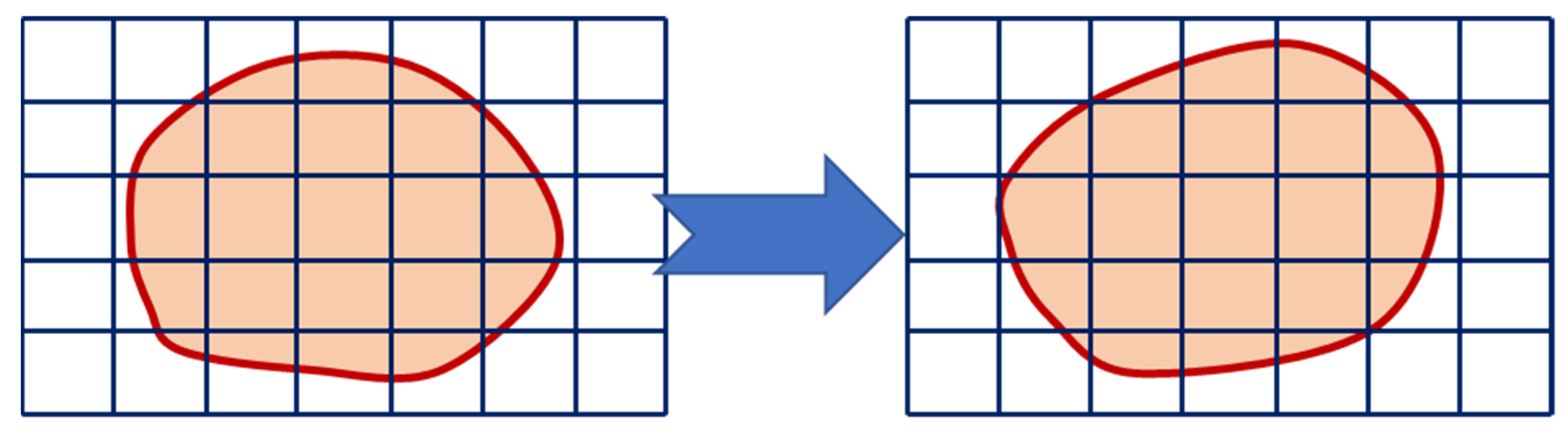
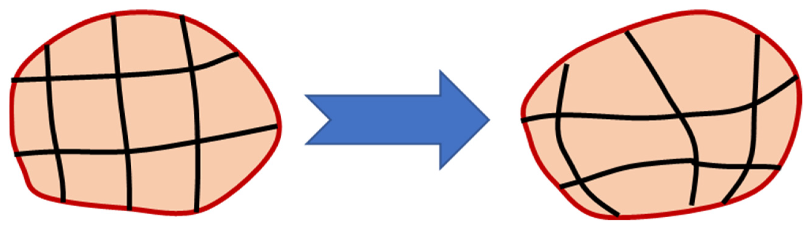
- The Lagrangian description (vj = ) states that the material and mesh are interconnected.
- 2.
- Eulerian description ( = 0): the mesh is fixed.
3. Validation of Numerical Model Using Experimental Date
4. Temperature Distribution
- The first is the experimental temperature measurement using instruments such as thermocouples in the welding area.
- The second approach is estimating the temperature in the welding area according to the microstructures formed after welding.
- The third method is to use models or process simulations to calculate the temperature. The use of this method is less challenging than the first and second approaches, and a large part of the research has used this method. The following is a review of each of these methods.
5. Strain Distribution
6. The Role of the Residual Stress
7. Forces and Torque during FSW Processing
- The vertical position of the tool;
- The force applied to the tool, which causes a change in the position of the tool.
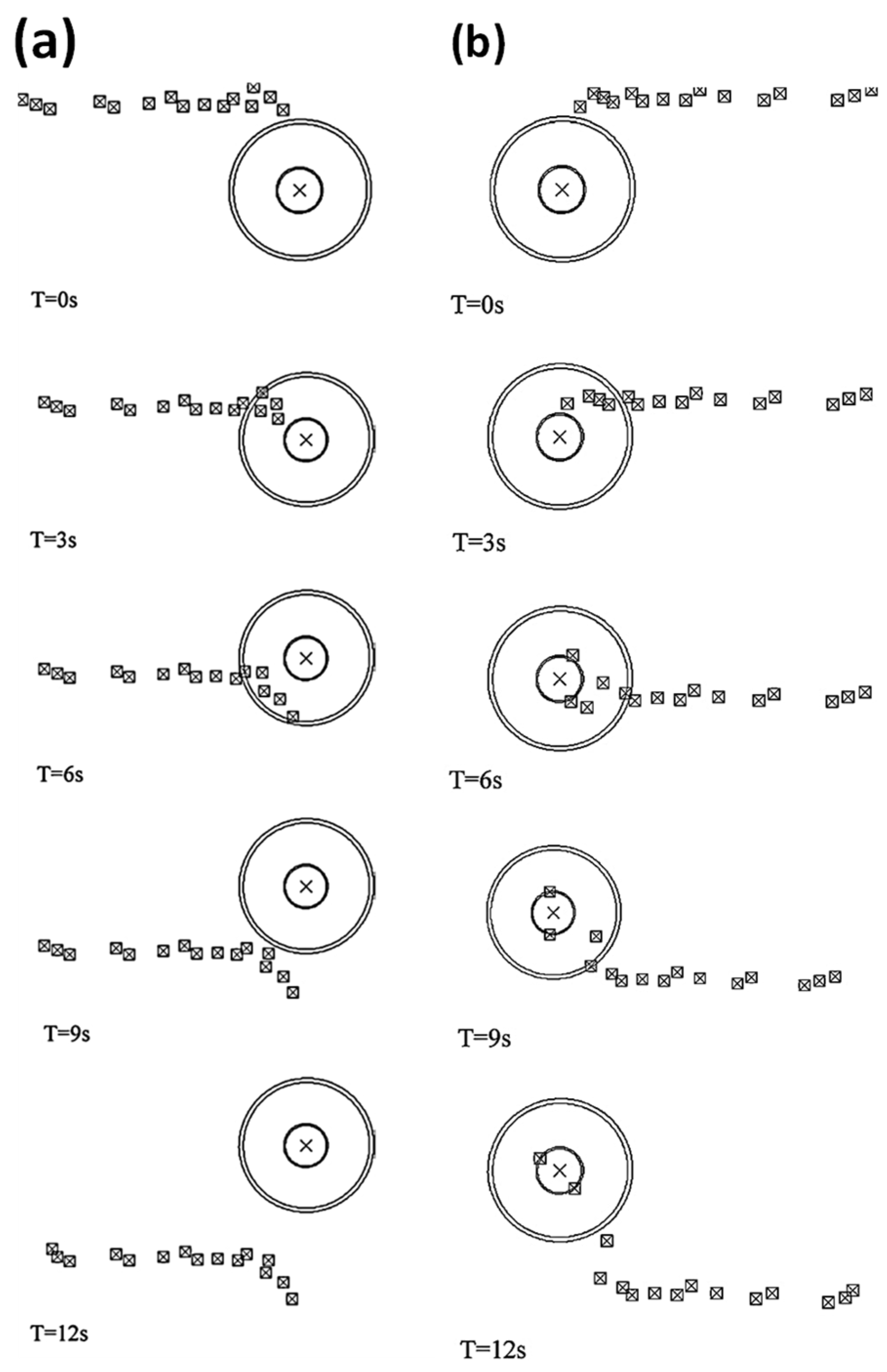
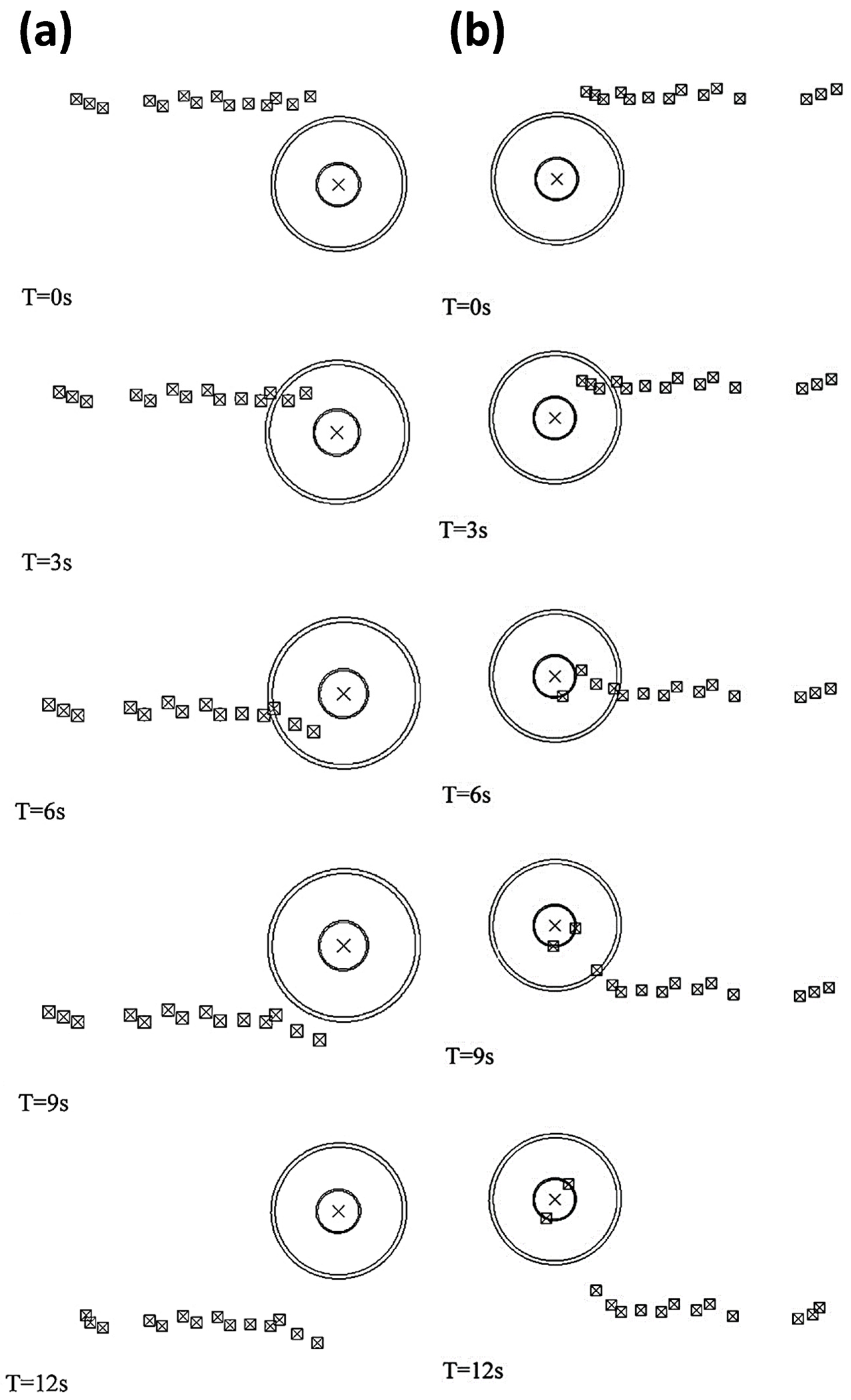
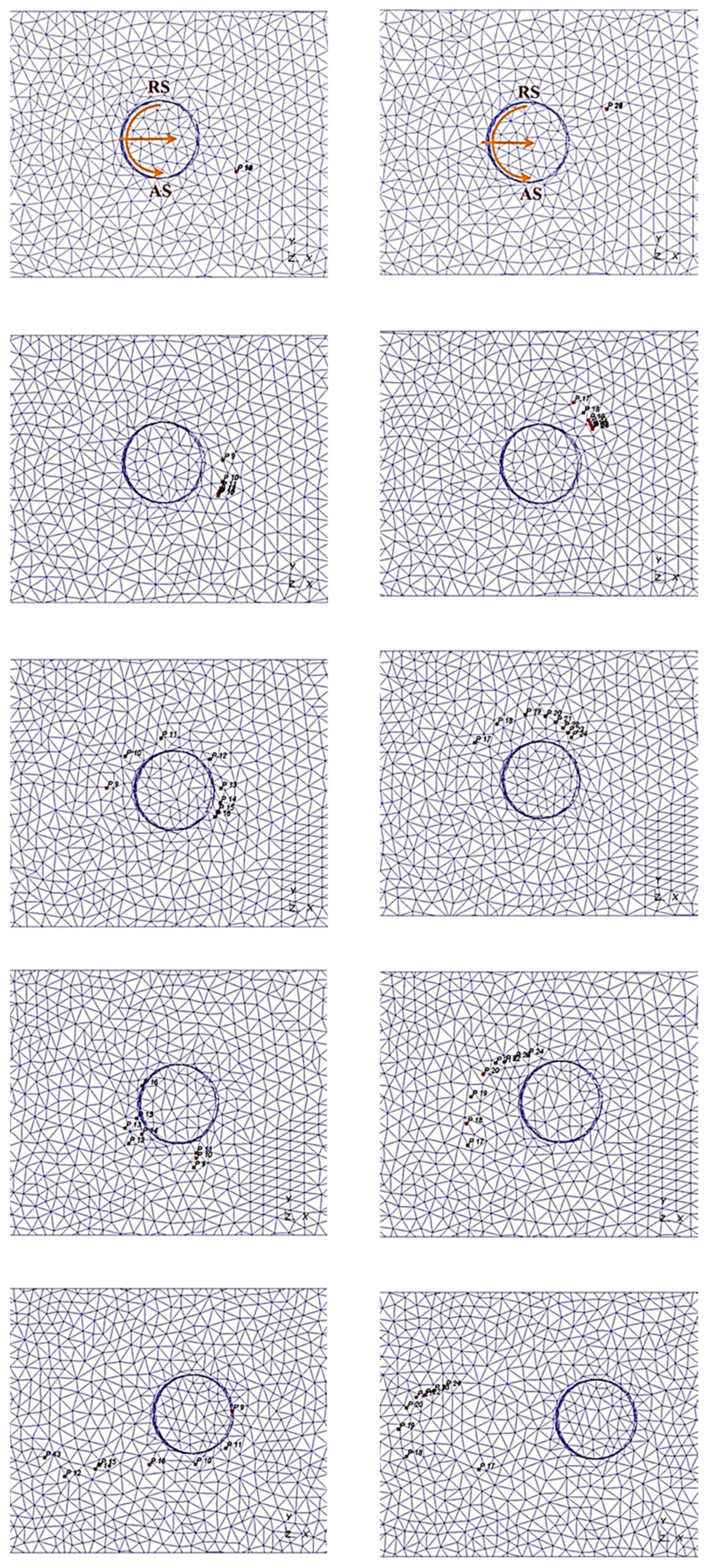
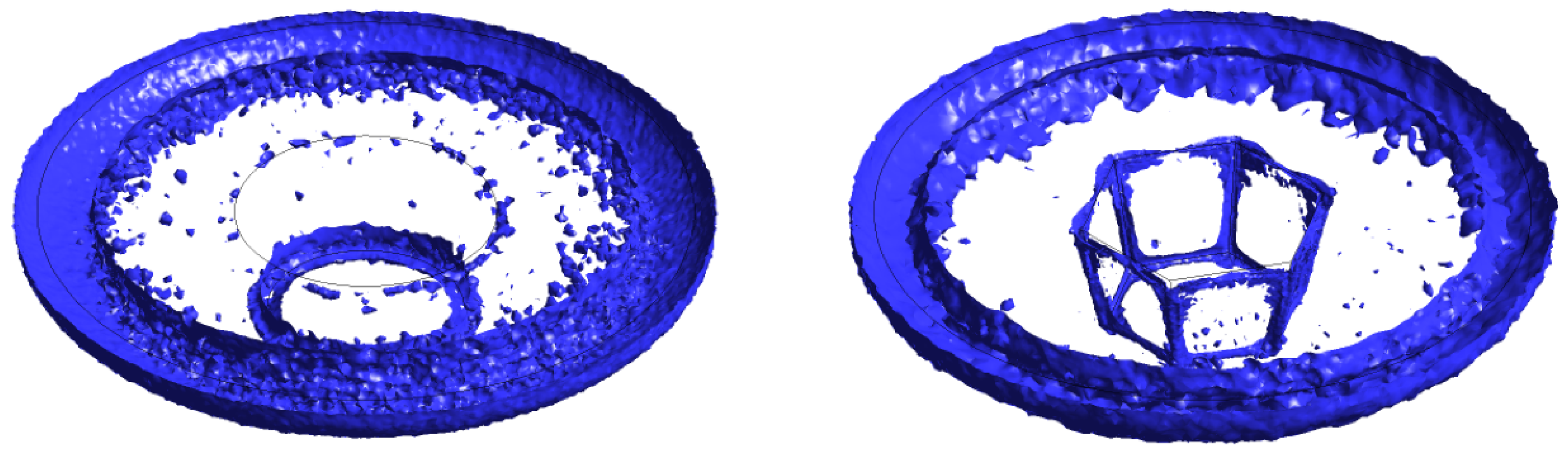
8. Material Flow during the FSW Process
9. Defect Prediction Using the Numerical Method
10. Microstructural Modeling and Simulation
- Molecular dynamics models;
- Precipitation modeling;
- Grain evolution modeling.
10.1. Molecular Dynamics (MD) Models
10.2. Precipitate Size Distribution (PSD) Models
10.3. Grain Evolution (GE) Modeling
- (i)
- Material models based on physical properties and evolution laws such as DDRX, CDRX, or GDRX models;
- (ii)
- Empirical methods commonly used in cellular automaton–finite element (CAFE) models but require extensive calibration steps;
- (iii)
- Monte Carlo methods consider final observations as a possible evolution through stochastic simulation.
11. Optimization of FSW Based on Residual Stress Modeling
12. Summary Conclusions
Funding
Data Availability Statement
Conflicts of Interest
Nomenclature
| ALE | Arbitrary Lagrangian–Eulerian |
| AS | Advancing side |
| BSS | Boundary shear stress |
| BV | Boundary velocity |
| CA | Cellular automaton |
| CDRX | Continuous dynamic recrystallization |
| CEL | Coupled Eulerian–Lagrangian |
| CFD | Computational fluid dynamics |
| CFSW | Conventional friction stir welding |
| SM | Computational solid mechanics |
| DDRX | Discontinuous dynamic recrystallization |
| DRX | Dynamic recrystallization |
| FE | Finite element |
| FEM | Finite element method |
| FGM | Functionally graded material |
| FSP | Friction stir processing |
| FSSW | Friction stir spot weld |
| FSW | Friction stir welding |
| FVM | Finite volume method |
| GDRX | Geometric dynamic recrystallization |
| HAGBs | High angle grain boundaries |
| HAZ | Heat-affected zone |
| LAGBs | Low angle grain boundaries |
| LCR | Longitudinal critically refracted |
| NZ | Nugget zone |
| PIV | Particle image velocimetry |
| RS | Retreating side |
| SFE | Stacking fault energy |
| SFSP | Submerged FSP |
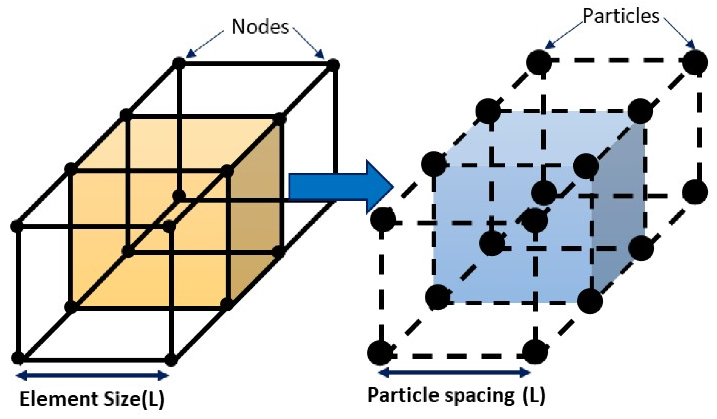
| SPH | Smoothed particle hydrodynamics |
| SZ | Stir zone |
| TMAZ | Thermomechanically affected zone |
| TWI | The Welding Institute |
| UFSW | Underwater friction stir welding |
| VOF | Volume of fluid |
| WZ | Welds zone |
References
- Khedr, M.; Hamada, A.; Järvenpää, A.; Elkatatny, S.; Abd-Elaziem, W. Review on the Solid-State Welding of Steels: Diffusion Bonding and Friction Stir Welding Processes. Metals 2023, 13, 54. [Google Scholar]
- Çam, G.; Javaheri, V.; Heidarzadeh, A. Advances in FSW and FSSW of dissimilar Al-alloy plates. J. Adhes. Sci. Technol. 2023, 37, 162–194. [Google Scholar]
- Sambasivam, S.; Gupta, N.; Singh, D.P.; Kumar, S.; Giri, J.M.; Gupta, M. A review paper of FSW on dissimilar materials using aluminum. Mater. Today Proc. 2023. [Google Scholar] [CrossRef]
- Zhang, Z.; Zhang, H.W. Numerical studies on the effect of transverse speed in friction stir welding. Mater. Des. 2009, 30, 900–907. [Google Scholar] [CrossRef]
- Aziz, S.B.; Dewan, M.W.; Huggett, D.J.; Wahab, M.A.; Okeil, A.M.; Liao, T.W. A Fully Coupled Thermomechanical Model of Friction Stir Welding (FSW) and Numerical Studies on Process Parameters of Lightweight Aluminum Alloy Joints. Acta Metall. Sin. Engl. Lett. 2018, 31, 1–18. [Google Scholar] [CrossRef]
- Zhang, Z.; Zhang, H.W. Numerical studies on controlling of process parameters in friction stir welding. J. Mater. Process. Technol. 2009, 209, 241–270. [Google Scholar] [CrossRef]
- Shojaeefard, M.; Akbari, M.; Asadi, P. Multi objective optimization of friction stir welding parameters using FEM and neural network. Int. J. Precis. Eng. Manuf. 2014, 15, 2351–2356. [Google Scholar] [CrossRef]
- Dialami, N.; Cervera, M.; Chiumenti, M. Effect of the Tool Tilt Angle on the Heat Generation and the Material Flow in Friction Stir Welding. Metals 2019, 9, 28. [Google Scholar]
- Aghajani Derazkola, H.; Kordani, N.; Aghajani Derazkola, H. Effects of friction stir welding tool tilt angle on properties of Al-Mg-Si alloy T-joint. CIRP J. Manuf. Sci. Technol. 2021, 33, 264–276. [Google Scholar] [CrossRef]
- Long, L.; Chen, G.; Zhang, S.; Liu, T.; Shi, Q. Finite-element analysis of the tool tilt angle effect on the formation of friction stir welds. J. Manuf. Process. 2017, 30, 562–569. [Google Scholar] [CrossRef]
- Meyghani, B.; Awang, M. The Influence of the Tool Tilt Angle on the Heat Generation and the Material Behavior in Friction Stir Welding (FSW). Metals 2022, 12, 1837. [Google Scholar]
- Marzbanrad, J.; Akbari, M.; Asadi, P.; Safaee, S. Characterization of the Influence of Tool Pin Profile on Microstructural and Mechanical Properties of Friction Stir Welding. Metall. Mater. Trans. B 2014, 45, 1887–1894. [Google Scholar] [CrossRef]
- Fourment, L.; Guerdoux, S. 3D numerical simulation of the three stages of Friction Stir Welding based on friction parameters calibration. Int. J. Mater. Form. 2008, 1, 1287–1290. [Google Scholar] [CrossRef]
- Kim, S.-D.; Yoon, J.-Y.; Na, S.-J. A study on the characteristics of FSW tool shapes based on CFD analysis. Weld World 2017, 61, 915–926. [Google Scholar] [CrossRef]
- Dialami, N.; Cervera, M.; Chiumenti, M.; Agelet de Saracibar, C. A fast and accurate two-stage strategy to evaluate the effect of the pin tool profile on metal flow, torque and forces in friction stir welding. Int. J. Mech. Sci. 2017, 122, 215–227. [Google Scholar] [CrossRef]
- Ghiasvand, A.; Hassanifard, S. Numerical simulation of FSW and FSSW with pinless tool of AA6061-T6 Al alloy by CEL approach. J. Solid Fluid Mech. 2018, 8, 65–75. [Google Scholar] [CrossRef]
- Malik, V.; Sanjeev, N.K.; Hebbar, H.S.; Kailas, S.V. Investigations on the Effect of Various Tool Pin Profiles in Friction Stir Welding Using Finite Element Simulations. Procedia Eng. 2014, 97, 1060–1068. [Google Scholar] [CrossRef]
- Chupradit, S.; Bokov, D.O.; Suksatan, W.; Landowski, M.; Fydrych, D.; Abdullah, M.E.; Derazkola, H.A. Pin Angle Thermal Effects on Friction Stir Welding of AA5058 Aluminum Alloy: CFD Simulation and Experimental Validation. Materials 2021, 14, 7565. [Google Scholar] [PubMed]
- Ghiasvand, A.; Kazemi, M.; Mahdipour Jalilian, M.; Ahmadi Rashid, H. Effects of tool offset, pin offset, and alloys position on maximum temperature in dissimilar FSW of AA6061 and AA5086. Int. J. Mech. Mater. Eng. 2020, 15, 6. [Google Scholar] [CrossRef]
- Aghajani Derazkola, H.; Simchi, A. Experimental and thermomechanical analysis of the effect of tool pin profile on the friction stir welding of poly(methyl methacrylate) sheets. J. Manuf. Process. 2018, 34, 412–423. [Google Scholar] [CrossRef]
- Hasan, A.F.; Bennett, C.J.; Shipway, P.H. A numerical comparison of the flow behaviour in Friction Stir Welding (FSW) using unworn and worn tool geometries. Mater. Des. 2015, 87, 1037–1046. [Google Scholar] [CrossRef]
- Shirvanimoghaddam, K.; Khayyam, H.; Abdizadeh, H.; Karbalaei Akbari, M.; Pakseresht, A.H.; Abdi, F.; Abbasi, A.; Naebe, M. Effect of B4C, TiB2 and ZrSiO4 ceramic particles on mechanical properties of aluminium matrix composites: Experimental investigation and predictive modelling. Ceram. Int. 2016, 42, 6206–6220. [Google Scholar] [CrossRef]
- Shirvanimoghaddam, K.; Khayyam, H.; Abdizadeh, H.; Karbalaei Akbari, M.; Pakseresht, A.H.; Ghasali, E.; Naebe, M. Boron carbide reinforced aluminium matrix composite: Physical, mechanical characterization and mathematical modelling. Mater. Sci. Eng. A 2016, 658, 135–149. [Google Scholar] [CrossRef]
- Shojaeefard, M.H.; Akbari, M.; Asadi, P.; Khalkhali, A. The effect of reinforcement type on the microstructure, mechanical properties, and wear resistance of A356 matrix composites produced by FSP. Int. J. Adv. Manuf. Technol. 2016, 91, 1391–1407. [Google Scholar] [CrossRef]
- Shojaeefard, M.H.; Akbari, M.; Khalkhali, A.; Asadi, P. Effect of tool pin profile on distribution of reinforcement particles during friction stir processing of B4C/aluminum composites. Proc. Inst. Mech. Eng. Part L J. Mater. Des. Appl. 2016, 232, 637–651. [Google Scholar] [CrossRef]
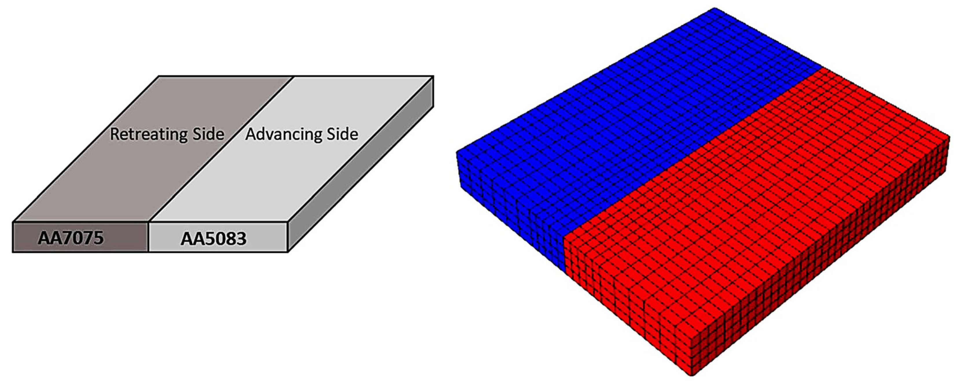
- Akbari, M.; Rahimi Asiabaraki, H.; Hassanzadeh, E.; Esfandiar, M. Simulation of dissimilar friction stir welding of AA7075 and AA5083 aluminium alloys using Coupled Eulerian–Lagrangian approach. Weld. Int. 2023, 37, 174–184. [Google Scholar] [CrossRef]
- Akbari, M.; Asiabaraki, H.R.; Aliha, M.R.M. Investigation of the effect of welding and rotational speed on strain and temperature during friction stir welding of AA5083 and AA7075 using the CEL approach. Eng. Res. Express 2023, 5, 025012. [Google Scholar] [CrossRef]
- Mishra, R.S.; Ma, Z.Y. Friction stir welding and processing. Mater. Sci. Eng. R Rep. 2005, 50, 1–78. [Google Scholar] [CrossRef]
- Khalaf, H.I.; Al-Sabur, R.; Abdullah, M.E.; Kubit, A.; Derazkola, H.A. Effects of Underwater Friction Stir Welding Heat Generation on Residual Stress of AA6068-T6 Aluminum Alloy. Materials 2022, 15, 2223. [Google Scholar] [CrossRef]
- Gadakh, V.S.; Adepu, K. Heat generation model for taper cylindrical pin profile in FSW. J. Mater. Res. Technol. 2013, 2, 370–375. [Google Scholar] [CrossRef]
- Terasaki, T.; Akiyama, T. Mechanical Behaviour of Joints in FSW: Residual Stress, Inherent Strain and Heat Input Generated by Friction Stir Welding. Weld World 2003, 47, 24–31. [Google Scholar] [CrossRef]
- Akbari, M.; Rahimi Asiabaraki, H. Modeling and optimization of tool parameters in friction stir lap joining of aluminum using RSM and NSGA II. Weld. Int. 2023, 37, 21–33. [Google Scholar] [CrossRef]
- Krasnowski, K.; Hamilton, C.; Dymek, S. Influence of the tool shape and weld configuration on microstructure and mechanical properties of the Al 6082 alloy FSW joints. Arch. Civ. Mech. Eng. 2015, 15, 133–141. [Google Scholar] [CrossRef]
- Sadoun, A.M.; Wagih, A.; Fathy, A.; Essa, A.R.S. Effect of tool pin side area ratio on temperature distribution in friction stir welding. Results Phys. 2019, 15, 102814. [Google Scholar] [CrossRef]
- Akbari, M.; Ezzati, M.; Asadi, P. Investigation of the effect of tool probe profile on reinforced particles distribution using experimental and CEL approaches. Int. J. Lightweight Mater. Manuf. 2022, 5, 213–223. [Google Scholar] [CrossRef]
- Das, S.S.; Raja, A.R.; Nautiyal, H.; Gautam, R.K.S.; Jha, P.; Sharma, J.; Singh, S. A Review on Aluminum Matrix Composites Synthesized by FSP. Macromol. Symp. 2023, 407, 2200119. [Google Scholar]
- Akbari, M.; Asadi, P.; Aliha, M.; Berto, F. Modeling and Optimization of Process Parameters of the Piston Alloy-Based Composite Produced by Fsp Using Response Surface Methodology. Surf. Rev. Lett. 2023, 30, 2350041. [Google Scholar]
- Asadi, P.; Akbari, M.; Karimi-Nemch, H. 12-Simulation of friction stir welding and processing. In Advances in Friction-Stir Welding and Processing; Givi, M.K.B., Asadi, P., Eds.; Woodhead Publishing: Cambridge, UK, 2014; pp. 499–542. [Google Scholar] [CrossRef]
- Colegrove, P.; Shercliff, H. Two-dimensional CFD modelling of flow round profiled FSW tooling. Sci. Technol. Weld. Join. 2004, 9, 483–492. [Google Scholar] [CrossRef]
- Pal, S.; Phaniraj, M. Determination of heat partition between tool and workpiece during FSW of SS304 using 3D CFD modeling. J. Mater. Process. Technol. 2015, 222, 280–286. [Google Scholar]
- Hasan, A. CFD modelling of friction stir welding (FSW) process of AZ31 magnesium alloy using volume of fluid method. J. Mater. Res. Technol. 2019, 8, 1819–1827. [Google Scholar]
- Savaş, A. Investigating the influence of tool shape during FSW of aluminum alloy via CFD analysis. J. Chin. Inst. Eng. 2016, 39, 211–220. [Google Scholar] [CrossRef]
- Colegrove, P.A.; Shercliff, H.R. 3-Dimensional CFD modelling of flow round a threaded friction stir welding tool profile. J. Mater. Process. Technol. 2005, 169, 320–327. [Google Scholar] [CrossRef]
- Chen, G.; Ma, Q.; Zhang, S.; Wu, J.; Zhang, G.; Shi, Q. Computational fluid dynamics simulation of friction stir welding: A comparative study on different frictional boundary conditions. J. Mater. Sci. Technol. 2018, 34, 128–134. [Google Scholar]
- Chen, G.; Feng, Z.; Zhu, Y.; Shi, Q. An alternative frictional boundary condition for computational fluid dynamics simulation of friction stir welding. J. Mater. Eng. Perform. 2016, 25, 4016–4023. [Google Scholar]
- Mohan, R.; Jayadeep, U.; Manu, R. CFD modelling of ultra-high rotational speed micro friction stir welding. J. Manuf. Process. 2021, 64, 1377–1386. [Google Scholar]
- Chen, G.; Shi, Q.; Zhang, S. Recent development and applications of CFD simulation for friction stir welding. In CFD Modeling and Simulation in Materials Processing; Springer: Berlin/Heidelberg, Germany, 2018; pp. 113–118. [Google Scholar]
- Kumar, R.R.; Kumar, A.; Kumar, A.; Ansu, A.K.; Goyal, A.; Saxena, K.K.; Prakash, C.; Prasad, J.L. Thermal simulation on friction stir welding of AA6061 aluminum alloy by computational fluid dynamics. Int. J. Interact. Des. Manuf. IJIDeM 2023, 1–11. [Google Scholar] [CrossRef]
- Myung, D.; Noh, W.; Kim, J.-H.; Kong, J.; Hong, S.-T.; Lee, M.-G. Probing the Mechanism of Friction Stir Welding with ALE Based Finite Element Simulations and Its Application to Strength Prediction of Welded Aluminum. Met. Mater. Int. 2021, 27, 650–666. [Google Scholar] [CrossRef]
- Jain, R.; Pal, S.K.; Singh, S.B. Finite Element Simulation of Temperature and Strain Distribution during Friction Stir Welding of AA2024 Aluminum Alloy. J. Inst. Eng. India Ser. C 2017, 98, 37–43. [Google Scholar] [CrossRef]
- Gök, K.; Aydin, M. Investigations of friction stir welding process using finite element method. Int. J. Adv. Manuf. Technol. 2013, 68, 775–780. [Google Scholar] [CrossRef]
- Fratini, L.; Buffa, G.; Palmeri, D.; Hua, J.; Shivpuri, R. Material flow in FSW of AA7075–T6 butt joints: Numerical simulations and experimental verifications. Sci. Technol. Weld. Join. 2006, 11, 412–421. [Google Scholar] [CrossRef]
- Akbari, M.; Asadi, P. Optimization of microstructural and mechanical properties of friction stir welded A356 pipes using Taguchi method. Mater. Res. Express 2019, 6, 066545. [Google Scholar] [CrossRef]
- Chinna Rao, J.T.; Harikiran, V.; Gurudatta, K.S.S.; Kumar Raju, M.V.D. Temperature and strain distribution during friction stir welding of AA6061 and AA5052 aluminum alloy using deform 3D. Mater. Today Proc. 2022, 59, 576–582. [Google Scholar] [CrossRef]
- Buffa, G.; Fratini, L.; Micari, F.; Shivpuri, R. Material Flow in FSW of T-joints: Experimental and Numerical Analysis. Int. J. Mater. Form. 2008, 1, 1283–1286. [Google Scholar] [CrossRef]
- Buffa, G.; Hua, J.; Shivpuri, R.; Fratini, L. Design of the friction stir welding tool using the continuum based FEM model. Mater. Sci. Eng. A 2006, 419, 381–388. [Google Scholar] [CrossRef]
- Asadi, P.; Besharati Givi, M.K.; Akbari, M. Microstructural simulation of friction stir welding using a cellular automaton method: A microstructure prediction of AZ91 magnesium alloy. Int. J. Mech. Mater. Eng. 2015, 10, 20. [Google Scholar] [CrossRef]
- Buffa, G.; Hua, J.; Shivpuri, R.; Fratini, L. A continuum based fem model for friction stir welding—Model development. Mater. Sci. Eng. A 2006, 419, 389–396. [Google Scholar] [CrossRef]
- Trimble, D.; Monaghan, J.; O’Donnell, G.E. Force generation during friction stir welding of AA2024-T3. CIRP Ann. 2012, 61, 9–12. [Google Scholar] [CrossRef]
- Pashazadeh, H.; Teimournezhad, J.; Masoumi, A. Numerical investigation on the mechanical, thermal, metallurgical and material flow characteristics in friction stir welding of copper sheets with experimental verification. Mater. Des. 2014, 55, 619–632. [Google Scholar] [CrossRef]
- Buffa, G.; Fratini, L.; Shivpuri, R. CDRX modelling in friction stir welding of AA7075-T6 aluminum alloy: Analytical approaches. J. Mater. Process. Technol. 2007, 191, 356–359. [Google Scholar] [CrossRef]
- Fratini, L.; Macaluso, G.; Pasta, S. Residual stresses and FCP prediction in FSW through a continuous FE model. J. Mater. Process. Technol. 2009, 209, 5465–5474. [Google Scholar] [CrossRef]
- Akbari, M.; Asadi, P. Dissimilar friction stir lap welding of aluminum to brass: Modeling of material mixing using coupled Eulerian–Lagrangian method with experimental verifications. Proc. Inst. Mech. Eng. Part L J. Mater. Des. Appl. 2020, 234, 1117–1128. [Google Scholar] [CrossRef]
- Bhattacharjee, R.; Datta, S.; Hammad, A.; Biswas, P. Prediction of various defects and material flow behavior during dissimilar FSW of DH36 shipbuilding steel and marine grade AA5083 using FE-based CEL approach. Model. Simul. Mater. Sci. Eng. 2023, 31, 035004. [Google Scholar]
- Asadi, P.; Mirzaei, M.; Akbari, M. Modeling of pin shape effects in bobbin tool FSW. Int. J. Lightweight Mater. Manuf. 2022, 5, 162–177. [Google Scholar] [CrossRef]
- Raut, N.; Yakkundi, V.; Vartak, A. A numerical technique to analyze the trend of temperature distribution in the friction stir welding process for titanium Ti 6Al 4V. Mater. Today Proc. 2021, 41, 329–334. [Google Scholar]
- Malik, V.; Sanjeev, N.; Hebbar, H.S.; Kailas, S.V. Time efficient simulations of plunge and dwell phase of FSW and its significance in FSSW. Procedia Mater. Sci. 2014, 5, 630–639. [Google Scholar]
- Grujicic, M.; Yavari, R.; Ramaswami, S.; Snipes, J.; Galgalikar, R. Computational analysis of inter-material mixing and weld-flaw formation during dissimilar-filler-metal friction stir welding (FSW). Multidiscip. Model. Mater. Struct. 2015, 11, 322–349. [Google Scholar]
- Iordache, M.D.; Badulescu, C.; Diakhate, M.; Constantin, M.A.; Nitu, E.L.; Demmouche, Y.; Dhondt, M.; Negrea, D. A numerical strategy to identify the FSW process optimal parameters of a butt-welded joint of quasi-pure copper plates: Modeling and experimental validation. Int. J. Adv. Manuf. Technol. 2021, 115, 2505–2520. [Google Scholar]
- Das, D.; Bag, S.; Pal, S.; Sharma, A. Material Defects in Friction Stir Welding through Thermo–Mechanical Simulation: Dissimilar Materials with Tool Wear Consideration. Materials 2023, 16, 301. [Google Scholar]
- Salloomi, K.N. Defect monitoring in dissimilar friction stir welding of aluminum alloys using Coupled Eulerian-Lagrangian (CEL) finite element model. Adv. Mater. Process. Technol. 2022, 1–17. [Google Scholar]
- Raut, N.N.; Yakkundi, V.; Vartak, A.; Teli, S. Effect of Plunging and Dwelling Period on Temperature Profile and Energy Dissipation in FSSW and Its Relevance in FSW. In Proceedings of the International Conference on Intelligent Manufacturing and Automation: ICIMA, Mumbai, India, 27–28 March 2020; pp. 211–220. [Google Scholar]
- Chalurkar, C.; Shukla, D.K. Temperature Analysis of Friction Stir Welding (AA6061-T6) with Coupled Eulerian-Lagrangian Approach. IOP Conf. Ser. Mater. Sci. Eng. 2022, 1248, 012035. [Google Scholar]
- Salih, O.S.; Ou, H.; Sun, W. Heat generation, plastic deformation and residual stresses in friction stir welding of aluminium alloy. Int. J. Mech. Sci. 2023, 238, 107827. [Google Scholar] [CrossRef]
- Salloomi, K.N.; Al-Sumaidae, S. Coupled Eulerian–Lagrangian prediction of thermal and residual stress environments in dissimilar friction stir welding of aluminum alloys. J. Adv. Join. Process. 2021, 3, 100052. [Google Scholar] [CrossRef]
- Teng, L.; Lu, X.; Luan, Y.; Sun, S. Predicting axial force in friction stir welding thick 2219 aluminum alloy plate. Int. J. Adv. Manuf. Technol. 2023, 126, 1025–1034. [Google Scholar] [CrossRef]
- Ghiasvand, A.; Suksatan, W.; Tomków, J.; Rogalski, G.; Derazkola, H.A. Investigation of the Effects of Tool Positioning Factors on Peak Temperature in Dissimilar Friction Stir Welding of AA6061-T6 and AA7075-T6 Aluminum Alloys. Materials 2022, 15, 702. [Google Scholar] [CrossRef]
- Iordache, M.; Nitu, E.; Bădulescu, C.; Iacomi, D.; Boţilă, L.N.; Radu, B. Evaluation of Thermal Distribution in Friction Stir Welding on Dissimilar Materials (Cu-Al) Using Infrared Thermography and Numerical Simulation. Adv. Mater. Res. 2016, 1138, 113–118. [Google Scholar] [CrossRef]
- Ajri, A.; Shin, Y.C. Investigation on the effects of process parameters on defect formation in friction stir welded samples via predictive numerical modeling and experiments. J. Manuf. Sci. Eng. 2017, 139, 111009. [Google Scholar] [CrossRef]
- Akbari, M.; Asadi, P.; Behnagh, R.A. Modeling of material flow in dissimilar friction stir lap welding of aluminum and brass using coupled Eulerian and Lagrangian method. Int. J. Adv. Manuf. Technol. 2021, 113, 721–734. [Google Scholar] [CrossRef]
- Al-Badour, F.; Merah, N.; Shuaib, A.; Bazoune, A. Coupled Eulerian Lagrangian finite element modeling of friction stir welding processes. J. Mater. Process. Technol. 2013, 213, 1433–1439. [Google Scholar] [CrossRef]
- Ragab, M.; Liu, H.; Yang, G.-J.; Ahmed, M.M. Friction stir welding of 1Cr11Ni2W2MoV martensitic stainless steel: Numerical simulation based on coupled Eulerian Lagrangian approach supported with experimental work. Appl. Sci. 2021, 11, 3049. [Google Scholar] [CrossRef]
- Das, D.; Bag, S.; Pal, S. Investigating surface defect by tool-material interaction in friction stir welding using coupled Eulerian-Lagrangian approach. Manuf. Lett. 2021, 30, 23–26. [Google Scholar] [CrossRef]
- Choudhary, A.K.; Jain, R. Numerical prediction of various defects and their formation mechanism during friction stir welding using coupled Eulerian-Lagrangian technique. Mech. Adv. Mater. Struct. 2022, 30, 2371–2384. [Google Scholar] [CrossRef]
- Nandan, R.; Roy, G.G.; Lienert, T.J.; Debroy, T. Three-dimensional heat and material flow during friction stir welding of mild steel. Acta Mater. 2007, 55, 883–895. [Google Scholar] [CrossRef]
- Liu, X.; Chen, G.; Ni, J.; Feng, Z. Computational Fluid Dynamics Modeling on Steady-State Friction Stir Welding of Aluminum Alloy 6061 to TRIP Steel. J. Manuf. Sci. Eng. 2016, 139, 051004. [Google Scholar] [CrossRef]
- Tiwari, A.; Pankaj, P.; Suman, S.; Biswas, P. CFD Modelling of Temperature Distribution and Material Flow Investigation during FSW of DH36 Shipbuilding Grade Steel. Trans. Indian Inst. Met. 2020, 73, 2291–2307. [Google Scholar] [CrossRef]
- Yang, C.; Wu, C.; Gao, S. Computational fluid dynamics model of AA6061 friction stir welding with considering mechanical anisotropy. Mater. Today Commun. 2022, 32, 103991. [Google Scholar] [CrossRef]
- Pankaj, P.; Tiwari, A.; Dhara, L.N.; Biswas, P. Multiphase CFD simulation and experimental investigation of friction stir welded high strength shipbuilding steel and aluminum alloy. CIRP J. Manuf. Sci. Technol. 2022, 39, 37–69. [Google Scholar] [CrossRef]
- Yang, C.; Wu, C.; Shi, L. Modeling the dissimilar material flow and mixing in friction stir welding of aluminum to magnesium alloys. J. Alloys Compd. 2020, 843, 156021. [Google Scholar] [CrossRef]
- Kadian, A.K.; Biswas, P. The study of material flow behaviour in dissimilar material FSW of AA6061 and Cu-B370 alloys plates. J. Manuf. Process. 2018, 34, 96–105. [Google Scholar] [CrossRef]
- Bokov, D.O.; Jawad, M.A.; Suksatan, W.; Abdullah, M.E.; Świerczyńska, A.; Fydrych, D.; Derazkola, H.A. Effect of pin shape on thermal history of aluminum-steel friction stir welded joint: Computational fluid dynamic modeling and validation. Materials 2021, 14, 7883. [Google Scholar] [CrossRef]
- Zhang, X.; Shi, L.; Wu, C.; Yang, C.; Gao, S. Multi-phase modelling of heat and mass transfer during Ti/Al dissimilar friction stir welding process. J. Manuf. Process. 2023, 94, 240–254. [Google Scholar] [CrossRef]
- Jiang, T.; Wu, C.; Shi, L. Effects of tool pin thread on temperature field and material mixing in friction stir welding of dissimilar Al/Mg alloys. J. Manuf. Process. 2022, 74, 112–122. [Google Scholar] [CrossRef]
- Yang, C.; Wu, C.; Shi, L. Analysis of friction reduction effect due to ultrasonic vibration exerted in friction stir welding. J. Manuf. Process. 2018, 35, 118–126. [Google Scholar] [CrossRef]
- Sadeghian, B.; Taherizadeh, A.; Atapour, M. Simulation of weld morphology during friction stir welding of aluminum-stainless steel joint. J. Mater. Process. Technol. 2018, 259, 96–108. [Google Scholar] [CrossRef]
- Carlone, P.; Palazzo, G.S. Influence of process parameters on microstructure and mechanical properties in AA2024-T3 friction stir welding. Metallogr. Microstruct. Anal. 2013, 2, 213–222. [Google Scholar] [CrossRef]
- Zhai, M.; Wu, C.; Su, H. Influence of tool tilt angle on heat transfer and material flow in friction stir welding. J. Manuf. Process. 2020, 59, 98–112. [Google Scholar] [CrossRef]
- Su, H.; Wu, C.-S. Numerical simulation for the comparison of thermal and plastic material flow behavior between symmetrical and asymmetrical boundary conditions during friction stir welding. Adv. Manuf. 2023, 11, 143–157. [Google Scholar] [CrossRef]
- He, H.; Liu, Z.; Zhu, Y.; Chu, J.; Li, S.; Pei, S.; Zhang, C.; Fu, A.; Zhao, W. Mechanism of pin thread and flat features affecting material thermal flow behaviours and mixing in Al-Cu dissimilar friction stir welding. Int. J. Mech. Sci. 2023, 260, 108615. [Google Scholar] [CrossRef]
- Gould, J.E.; Feng, Z. Heat flow model for friction stir welding of aluminum alloys. J. Mater. Process. Manuf. Sci. 1998, 7, 185–194. [Google Scholar] [CrossRef]
- Shojaeefard, M.H.; Khalkhali, A.; Akbari, M.; Asadi, P. Investigation of friction stir welding tool parameters using FEM and neural network. Proc. Inst. Mech. Eng. Part L J. Mater. Des. Appl. 2013, 229, 209–217. [Google Scholar] [CrossRef]
- Buffa, G.; Ducato, A.; Fratini, L. FEM based prediction of phase transformations during Friction Stir Welding of Ti6Al4V titanium alloy. Mater. Sci. Eng. A 2013, 581, 56–65. [Google Scholar] [CrossRef]
- Dong, P.; Lu, F.; Hong, J.; Cao, Z. Coupled thermomechanical analysis of friction stir welding process using simplified models. Sci. Technol. Weld. Join. 2001, 6, 281–287. [Google Scholar] [CrossRef]
- Chao, Y.J.; Qi, X.; Tang, W. Heat transfer in friction stir welding—Experimental and numerical studies. J. Manuf. Sci. Eng. 2003, 125, 138–145. [Google Scholar] [CrossRef]
- Shi, Q.Y.; Wang, X.B.; Kang, X.; Sun, Y.J. Temperature fields during friction stir welding. J. Tsinghua Univ. 2010, 50, 980–983. [Google Scholar]
- Chen, C.; Kovacevic, R. Thermomechanical modelling and force analysis of friction stir welding by the finite element method. Proc. Inst. Mech. Eng. Part C J. Mech. Eng. Sci. 2004, 218, 509–519. [Google Scholar] [CrossRef]
- Akbari, M.; Aliha, M.R.M.; Berto, F. Investigating the role of different components of friction stir welding tools on the generated heat and strain. Forces Mech. 2023, 10, 100166. [Google Scholar] [CrossRef]
- Asadi, P.; Mahdavinejad, R.A.; Tutunchilar, S. Simulation and experimental investigation of FSP of AZ91 magnesium alloy. Mater. Sci. Eng. A 2011, 528, 6469–6477. [Google Scholar] [CrossRef]
- Aymone, J.L.F.; Bittencourt, E.; Creus, G.J. Simulation of 3D metal-forming using an arbitrary Lagrangian–Eulerian finite element method. J. Mater. Process. Technol. 2001, 110, 218–232. [Google Scholar] [CrossRef]
- Deng, X.; Xu, S. Two-dimensional finite element simulation of material flow in the friction stir welding process. J. Manuf. Process. 2004, 6, 125–133. [Google Scholar] [CrossRef]
- Schmidt, H.N.B.; Hattel, J. Modelling thermomechanical conditions at the tool/matrix interface in Friction Stir Welding. In 5th International Friction Stir Welding Symposium; The Welding Institute: Metz, France, 2004. [Google Scholar]
- Mandal, S.; Rice, J.; Elmustafa, A. Experimental and numerical investigation of the plunge stage in friction stir welding. J. Mater. Process. Technol. 2008, 203, 411–419. [Google Scholar] [CrossRef]
- Assidi, M.; Fourment, L. Accurate 3D friction stir welding simulation tool based on friction model calibration. Int. J. Mater. Form. 2009, 2, 327–330. [Google Scholar] [CrossRef]
- Asadi, P.; Akbari, M. Numerical modeling and experimental investigation of brass wire forming by friction stir back extrusion. Int. J. Adv. Manuf. Technol. 2021, 116, 3231–3245. [Google Scholar] [CrossRef]
- Ajri, A.; Shin, Y. Investigation on the Effects of Process Parameters on Defect Formation in Friction Stir Welded Samples via Predictive Numerical Modeling and Experiments; ASME: Atlanta, GA, USA, 2017; p. V001T002A008. [Google Scholar]
- Chen, K.; Liu, X.; Ni, J. Thermal-mechanical modeling on friction stir spot welding of dissimilar materials based on Coupled Eulerian-Lagrangian approach. Int. J. Adv. Manuf. Technol. 2017, 91, 1697–1707. [Google Scholar] [CrossRef]
- Chauhan, P.; Jain, R.; Pal, S.K.; Singh, S.B. Modeling of defects in friction stir welding using coupled Eulerian and Lagrangian method. J. Manuf. Process. 2018, 34, 158–166. [Google Scholar] [CrossRef]
- Al-Badour, F.; Merah, N.; Shuaib, A.; Bazoune, A. Thermo-mechanical finite element model of friction stir welding of dissimilar alloys. Int. J. Adv. Manuf. Technol. 2014, 72, 607–617. [Google Scholar] [CrossRef]
- Safari, M.; Joudaki, J. Coupled Eulerian-Lagrangian (CEL) Modeling of Material Flow in Dissimilar Friction Stir Welding of Aluminum Alloys. Iran. J. Mater. Form. 2019, 6, 10–19. [Google Scholar] [CrossRef]
- Lu, X.; Zhang, W.; Sun, X.; Sun, S.; Liang, S.Y. A study on temperature field and process of FSW thick 2219 aluminum alloy plate. J. Braz. Soc. Mech. Sci. Eng. 2023, 45, 326. [Google Scholar] [CrossRef]
- Ansari, M.A.; Abdi Behnagh, R. Numerical study of friction stir welding (FSW) plunging phase using smoothed particle hydrodynamics (SPH). Model. Simul. Mater. Sci. Eng. 2019, 27, 055006. [Google Scholar] [CrossRef]
- Kajtar, J.; Monaghan, J.J. SPH simulations of swimming linked bodies. J. Comput. Phys. 2008, 227, 8568–8587. [Google Scholar] [CrossRef]
- Pan, W.; Li, D.; Tartakovsky, A.M.; Ahzi, S.; Khraisheh, M.; Khaleel, M. A new smoothed particle hydrodynamics non-Newtonian model for friction stir welding: Process modeling and simulation of microstructure evolution in a magnesium alloy. Int. J. Plast. 2013, 48, 189–204. [Google Scholar] [CrossRef]
- Bagheri, B.; Abdollahzadeh, A.; Abbasi, M.; Kokabi, A.H. Numerical analysis of vibration effect on friction stir welding by smoothed particle hydrodynamics (SPH). Int. J. Adv. Manuf. Technol. 2020, 110, 209–228. [Google Scholar] [CrossRef]
- Bagheri, B.; Abbasi, M.; Abdolahzadeh, A.; Kokabi, A.H. Numerical analysis of cooling and joining speed effects on friction stir welding by smoothed particle hydrodynamics (SPH). Arch. Appl. Mech. 2020, 90, 2275–2296. [Google Scholar] [CrossRef]
- Shishova, E.; Panzer, F.; Werz, M.; Eberhard, P. Reversible inter-particle bonding in SPH for improved simulation of friction stir welding. Comput. Part. Mech. 2023, 10, 555–564. [Google Scholar] [CrossRef]
- Hannachi, N.; Khalfallah, A.; Leitão, C.; Rodrigues, D.M. Comparison Between ALE and CEL Finite Element Formulations to Simulate Friction Stir Spot Welding. In Advances in Mechanical Engineering and Mechanics II; Springer International Publishing: Cham, Switzerland, 2022; pp. 277–284. [Google Scholar]
- Hannachi, N.; Khalfallah, A.; Leitão, C.; Rodrigues, D. Thermo-mechanical modelling of the Friction Stir Spot Welding process: Effect of the friction models on the heat generation mechanisms. Proc. Inst. Mech. Eng. Part L J. Mater. Des. Appl. 2022, 236, 1464–1475. [Google Scholar] [CrossRef]
- Talebizadehsardari, P.; Musharavati, F.; Khan, A.; Sebaey, T.A.; Eyvaziana, A.; Derazkola, H.A. Underwater friction stir welding of Al-Mg alloy: Thermo-mechanical modeling and validation. Mater. Today Commun. 2021, 26, 101965. [Google Scholar] [CrossRef]
- Tutunchilar, S.; Haghpanahi, M.; Besharati Givi, M.K.; Asadi, P.; Bahemmat, P. Simulation of material flow in friction stir processing of a cast Al–Si alloy. Mater. Des. 2012, 40, 415–426. [Google Scholar] [CrossRef]
- Shojaeefard, M.H.; Akbari, M.; Khalkhali, A.; Asadi, P.; Parivar, A.H. Optimization of microstructural and mechanical properties of friction stir welding using the cellular automaton and Taguchi method. Mater. Des. 2014, 64, 660–666. [Google Scholar] [CrossRef]
- Schmidt, H.; Hattel, J.; Wert, J. An analytical model for the heat generation in friction stir welding. Model. Simul. Mater. Sci. Eng. 2004, 12, 143–157. [Google Scholar] [CrossRef]
- Anders, L.; Mathias, S.; Hattel, J.H. Estimating the workpiece-backing plate heat transfer coefficient in friction stirwelding. Eng. Comput. 2012, 29, 65–82. [Google Scholar] [CrossRef]
- Prasanna, P.; Rao, B.S.; Rao, G.K.M. Finite element modeling for maximum temperature in friction stir welding and its validation. Int. J. Adv. Manuf. Technol. 2010, 51, 925–933. [Google Scholar] [CrossRef]
- Xu, J.; Vaze, S.P.; Ritter, R.J.; Colligan, K.J.; Pickens, J.R. Experimental and numerical study of thermal process in friction stir welding. In Joining of Advanced and Specialty Materials VI; ASM International: Almere, The Netherlands, 2004; pp. 10–19. [Google Scholar]
- Awang, M.; Mucino, V.H. Energy generation during friction stir spot welding (FSSW) of Al 6061-T6 plates. Mater. Manuf. Process. 2010, 25, 167–174. [Google Scholar] [CrossRef]
- Kim, D.; Badarinarayan, H.; Kim, J.H.; Kim, C.; Okamoto, K.; Wagoner, R.; Chung, K. Numerical simulation of friction stir butt welding process for AA5083-H18 sheets. Eur. J. Mech. A Solids 2010, 29, 204–215. [Google Scholar] [CrossRef]
- Lü, S.; Yan, J.; Li, W.; Yang, S. Simulation on Temperature Field of Friction Stir Welded Joints of 2024-T4 Al. Acta Metall. Sin. Engl. Lett. 2005, 18, 552. [Google Scholar]
- Rajesh, S.; Bang, H.S.; Kim, H.J.; Bang, H.S. Analysis of complex heat flow phenomena with friction stir welding using 3D-analytical model. Adv. Mater. Res. 2007, 15, 339–344. [Google Scholar]
- Fraser, K.; Kiss, L.I.; St-Georges, L.; Drolet, D. Optimization of Friction Stir Weld Joint Quality Using a Meshfree Fully-Coupled Thermo-Mechanics Approach. Metals 2018, 8, 101. [Google Scholar] [CrossRef]
- Zhang, Z.; Bie, J.; Liu, Y.; Zhang, H. Effect of traverse/rotational speed on material deformations and temperature distributions in friction stir welding. J. Mater. Sci. Technol. 2008, 24, 907. [Google Scholar]
- Akbari, M.; Asadi, P. Effects of different cooling conditions on friction stir processing of A356 alloy: Numerical modeling and experiment. Proc. Inst. Mech. Eng. Part C J. Mech. Eng. Sci. 2021, 236, 4133–4146. [Google Scholar] [CrossRef]
- Besharati-Givi, M.-K.; Asadi, P. Advances in Friction-Stir Welding and Processing; Elsevier: Amsterdam, The Netherlands, 2014. [Google Scholar]
- Meena, S.L.; Murtaza, Q.; Walia, R.S.; Niranjan, M.S.; Tyagi, A. Modelling and simulation of FSW of polycarbonate using Finite element analysis. Mater. Today Proc. 2022, 50, 2424–2429. [Google Scholar] [CrossRef]
- Lemos, G.V.B.; Farina, A.B.; Nunes, R.M.; Cunha, P.H.C.P.d.; Bergmann, L.; Santos, J.F.d.; Reguly, A. Residual stress characterization in friction stir welds of alloy 625. J. Mater. Res. Technol. 2019, 8, 2528–2537. [Google Scholar] [CrossRef]
- Hattel, J.H.; Nielsen, K.L.; Tutum, C.C. The effect of post-welding conditions in friction stir welds: From weld simulation to ductile failure. Eur. J. Mech. A Solids 2012, 33, 67–74. [Google Scholar] [CrossRef]
- Threadgill, P.L.; Leonard, A.J.; Shercliff, H.R.; Withers, P.J. Friction stir welding of aluminium alloys. Int. Mater. Rev. 2009, 54, 49–93. [Google Scholar] [CrossRef]
- Hattel, J.H.; Sonne, M.R.; Tutum, C.C. Modelling residual stresses in friction stir welding of Al alloys—A review of possibilities and future trends. Int. J. Adv. Manuf. Technol. 2015, 76, 1793–1805. [Google Scholar] [CrossRef]
- Ge, Y.Z.; Sutton, M.A.; Deng, X.; Reynolds, A.P. Limited weld residual stress measurements in fatigue crack propagation: Part I. Complete field representation through least-squares finite-element smoothing. Fatigue Fract. Eng. Mater. Struct. 2006, 29, 524–536. [Google Scholar] [CrossRef]
- Richards, D.G.; Prangnell, P.B.; Withers, P.J.; Williams, S.W.; Nagy, T.; Morgan, S. Efficacy of active cooling for controlling residual stresses in friction stir welds. Sci. Technol. Weld. Join. 2010, 15, 156–165. [Google Scholar] [CrossRef]
- Lévesque, D.; Dubourg, L.; Blouin, A. Laser ultrasonics for defect detection and residual stress measurement of friction stir welds. Nondestruct. Test. Eval. 2011, 26, 319–333. [Google Scholar] [CrossRef]
- Carney, K.; Hatamleh, O.; Smith, J.; Matrka, T.; Gilat, A.; Hill, M.; Truong, C. A Numerical Simulation of the Residual Stresses in Laser-Peened Friction Stir-Welded Aluminum 2195 Joints. Int. J. Struct. Integr. 2011, 2, 62–73. [Google Scholar] [CrossRef]
- Deplus, K.; Simar, A.; Haver, W.V.; Meester, B.d. Residual stresses in aluminium alloy friction stir welds. Int. J. Adv. Manuf. Technol. 2011, 56, 493–504. [Google Scholar] [CrossRef]
- Riahi, M.; Nazari, H. Analysis of transient temperature and residual thermal stresses in friction stir welding of aluminum alloy 6061-T6 via numerical simulation. Int. J. Adv. Manuf. Technol. 2011, 55, 143–152. [Google Scholar] [CrossRef]
- Sadeghi, S.; Najafabadi, M.A.; Javadi, Y.; Mohammadisefat, M. Using ultrasonic waves and finite element method to evaluate through-thickness residual stresses distribution in the friction stir welding of aluminum plates. Mater. Des. 2013, 52, 870–880. [Google Scholar] [CrossRef]
- Kaid, M.; Zemri, M.; Brahami, A.; Zahaf, S. Effect of friction stir welding (FSW) parameters on the peak temperature and the residual stresses of aluminum alloy 6061-T6: Numerical modelisation. Int. J. Interact. Des. Manuf. IJIDeM 2019, 13, 797–807. [Google Scholar] [CrossRef]
- Shokri, V.; Sadeghi, A.; Sadeghi, M.H. Thermomechanical modeling of friction stir welding in a Cu-DSS dissimilar joint. J. Manuf. Process. 2018, 31, 46–55. [Google Scholar] [CrossRef]
- Geng, P.; Morimura, M.; Wu, S.; Liu, Y.; Ma, Y.; Ma, N.; Aoki, Y.; Fujii, H.; Ma, H.; Qin, G. Prediction of residual stresses within dissimilar Al/steel friction stir lap welds using an Eulerian-based modeling approach. J. Manuf. Process. 2022, 79, 340–355. [Google Scholar] [CrossRef]
- He, W.; Li, M.; Song, Q.; Liu, J.; Hu, W. Efficacy of External Stationary Shoulder for Controlling Residual Stress and Distortion in Friction Stir Welding. Trans. Indian Inst. Met. 2019, 72, 1349–1359. [Google Scholar] [CrossRef]
- Dubourg, L.; Doran, P.; Gharghouri, M.A.; Larose, S.; Jahazi, M. Prediction and measurements of thermal residual stresses in AA2024-T3 friction stir welds as a function of welding parameters. In Materials Science Forum; Trans Tech Publishers: Zurich, Switzerland, 2010; pp. 1215–1220. [Google Scholar]
- Aiping, Y.D.S.Q.W.; Silvanus, J. Numerical analysis on the functions of stir tool’s mechanical loads during friction stir welding. Acta Met. Sin. 2009, 45, 994–999. [Google Scholar]
- Jin, L.-Z.; Sandström, R. Numerical simulation of residual stresses for friction stir welds in copper canisters. J. Manuf. Process. 2012, 14, 71–81. [Google Scholar] [CrossRef]
- Bastier, A.; Maitournam, M.; Roger, F.; Van, K.D. Modelling of the residual state of friction stir welded plates. J. Mater. Process. Technol. 2008, 200, 25–37. [Google Scholar] [CrossRef]
- Eivani, A.R.; Vafaeenezhad, H.; Jafarian, H.R.; Zhou, J. A novel approach to determine residual stress field during FSW of AZ91 Mg alloy using combined smoothed particle hydrodynamics/neuro-fuzzy computations and ultrasonic testing. J. Magnes. Alloys 2021, 9, 1304–1328. [Google Scholar] [CrossRef]
- Zina, N.; Zahaf, S.; Bouaziz, S.A.; Brahami, A.; Kaid, M.; Chetti, B.; Najafi Vafa, Z. Numerical Simulation on the Effect of Friction Stir Welding Parameters on the Peak Temperature, Von Mises Stress, and Residual Stresses of 6061-T6 Aluminum Alloy. J. Fail. Anal. Prev. 2019, 19, 1698–1719. [Google Scholar] [CrossRef]
- Ranjole, C.; Singh, V.P.; Kuriachen, B.; Vineesh, K.P. Numerical Prediction and Experimental Investigation of Temperature, Residual Stress and Mechanical Properties of Dissimilar Friction-Stir Welded AA5083 and AZ31 Alloys. Arab. J. Sci. Eng. 2022, 47, 16103–16115. [Google Scholar] [CrossRef]
- Atharifar, H.; Lin, D.; Kovacevic, R. Numerical and Experimental Investigations on the Loads Carried by the Tool During Friction Stir Welding. J. Mater. Eng. Perform. 2009, 18, 339–350. [Google Scholar] [CrossRef]
- Ulysse, P. Three-dimensional modeling of the friction stir-welding process. Int. J. Mach. Tools Manuf. 2002, 42, 1549–1557. [Google Scholar] [CrossRef]
- Nandan, R.; Roy, G.G.; Lienert, T.J.; DebRoy, T. Numerical modelling of 3D plastic flow and heat transfer during friction stir welding of stainless steel. Sci. Technol. Weld. Join. 2006, 11, 526–537. [Google Scholar] [CrossRef]
- Rai, R.; De, A.; Bhadeshia, H.K.D.H.; DebRoy, T. Review: Friction stir welding tools. Sci. Technol. Weld. Join. 2011, 16, 325–342. [Google Scholar] [CrossRef]
- Arora, A.; De, A.; DebRoy, T. Toward optimum friction stir welding tool shoulder diameter. Scr. Mater. 2011, 64, 9–12. [Google Scholar] [CrossRef]
- Jain, R.; Pal, S.K.; Singh, S.B. Finite element simulation of pin shape influence on material flow, forces in friction stir welding. Int. J. Adv. Manuf. Technol. 2018, 94, 1781–1797. [Google Scholar] [CrossRef]
- Roy, B.S.; Saha, S.C.; Deb Barma, J. 3-D modeling & numerical simulation of friction stir welding process. Adv. Mater. Res. 2012, 488, 1189–1193. [Google Scholar]
- Idagawa, H.; Torres, E.; Ramirez, A. CFD modeling of dissimilar aluminum-steel friction stir welds. In Proceedings of the International Conference: Trends in Welding Research, Pine Mountain, GA, USA, 1 June–5 June 2013. [Google Scholar]
- Wang, G.; Zhu, L.; Zhang, Z. Modeling of material flow in friction stir welding process. China Weld. Engl. Version 2007, 16, 63–70. [Google Scholar]
- Ji, S.; Shi, Q.; Zhang, L.; Zou, A.; Gao, S.; Zan, L. Numerical simulation of material flow behavior of friction stir welding influenced by rotational tool geometry. Comput. Mater. Sci. 2012, 63, 218–226. [Google Scholar] [CrossRef]
- Shude, J.; Aili, Z.; Yumei, Y.; Guohong, L.; Yanye, J.; Fu, L. Numerical simulation of effect of rotational tool with screw on material flow behavior of friction stir welding of Ti6Al4V alloy. Acta Metall. Sin. Engl. Lett. 2012, 25, 365. [Google Scholar]
- Qin, D.Q.; Fu, L.; Shen, Z.K. Visualisation and numerical simulation of material flow behaviour during high-speed FSW process of 2024 aluminium alloy thin plate. Int. J. Adv. Manuf. Technol. 2019, 102, 1901–1912. [Google Scholar] [CrossRef]
- Su, H.; Wang, T.; Wu, C. Formation of the periodic material flow behaviour in friction stir welding. Sci. Technol. Weld. Join. 2021, 26, 286–293. [Google Scholar] [CrossRef]
- Luo, H.; Wu, T.; Wang, P.; Zhao, F.; Wang, H.; Li, Y. Numerical Simulation of Material Flow and Analysis of Welding Characteristics in Friction Stir Welding Process. Metals 2019, 9, 621. [Google Scholar] [CrossRef]
- Naumov, A.; Rylkov, E.; Polyakov, P.; Isupov, F.; Rudskoy, A.; Aoh, J.-N.; Popovich, A.; Panchenko, O. Effect of Different Tool Probe Profiles on Material Flow of Al–Mg–Cu Alloy Joined by Friction Stir Welding. Materials 2021, 14, 6296. [Google Scholar] [CrossRef]
- Buffa, G. Joining Ti6Al4V and AISI 304 through friction stir welding of lap joints: Experimental and numerical analysis. Int. J. Mater. Form. 2016, 9, 59–70. [Google Scholar] [CrossRef]
- Padmanaban, R.; Kishore, V.R.; Balusamy, V. Numerical Simulation of Temperature Distribution and Material Flow During Friction Stir Welding of Dissimilar Aluminum Alloys. Procedia Eng. 2014, 97, 854–863. [Google Scholar] [CrossRef]
- Mirzaei, M.; Asadi, P.; Fazli, A. Effect of Tool Pin Profile on Material Flow in Double Shoulder Friction Stir Welding of AZ91 Magnesium Alloy. Int. J. Mech. Sci. 2020, 183, 105775. [Google Scholar] [CrossRef]
- Liu, Q.; Han, R.; Gao, Y.; Ke, L. Numerical investigation on thermo-mechanical and material flow characteristics in friction stir welding for aluminum profile joint. Int. J. Adv. Manuf. Technol. 2021, 114, 2457–2469. [Google Scholar] [CrossRef]
- Hoßfeld, M. A Fully Coupled Thermomechanical 3D Model for All Phases of Friction Stir Welding; University of Stuttgart: Sttutgart, Germany, 2016. [Google Scholar]
- Guerdoux, S.; Fourment, L. A 3D numerical simulation of different phases of friction stir welding. Model. Simul. Mater. Sci. Eng. 2009, 17, 075001. [Google Scholar] [CrossRef]
- Chen, J.; Wang, X.; Shi, L.; Wu, C.; Liu, H.; Chen, G. Numerical simulation of weld formation in friction stir welding based on non-uniform tool-workpiece interaction: An effect of tool pin size. J. Manuf. Process. 2023, 86, 85–97. [Google Scholar] [CrossRef]
- Zhu, Y.; Chen, G.; Chen, Q.; Zhang, G.; Shi, Q. Simulation of material plastic flow driven by non-uniform friction force during friction stir welding and related defect prediction. Mater. Des. 2016, 108, 400–410. [Google Scholar] [CrossRef]
- Ajri, A.; Rohatgi, N.; Shin, Y.C. Analysis of defect formation mechanisms and their effects on weld strength during friction stir welding of Al 6061-T6 via experiments and finite element modeling. Int. J. Adv. Manuf. Technol. 2020, 107, 4621–4635. [Google Scholar] [CrossRef]
- Dmitriev, A.I.; Kolubaev, E.A.; Nikonov, A.Y.; Rubstob, V.E.; Psakhie, S.G. Study patterns of microstructure formation during friction stir welding. In Proceedings of the XLII International Summer School–Conference APM 2014, St. Petersburg, Russia, 30 June–5 July 2014. [Google Scholar]
- Nikonov, A.Y.; Dmitriev, A.I.; Konovalenko, I.S.; Kolubaev, E.A.; Astafurov, S.V.; Psakhie, S.G. Features of interface formation in crystallites under mechanically activated diffusion. A molecular dynamics study. In COMPLAS XIII: Proceedings of the XIII International Conference on Computational Plasticity: Fundamentals and Applications; CIMNE: Barcelona, Spain, 2015; pp. 982–991. [Google Scholar]
- Myhr, O.; Grong, Ø.; Klokkehaug, S.; Fjoer, H.; Kluken, A. Process model for welding of Al–Mg–Si extrusions Part 1: Precipitate stability. Sci. Technol. Weld. Join. 1997, 2, 245–253. [Google Scholar] [CrossRef]
- Frigaard, Ø.; Grong, Ø.; Midling, O. A process model for friction stir welding of age hardening aluminum alloys. Metall. Mater. Trans. A 2001, 32, 1189–1200. [Google Scholar] [CrossRef]
- Wagner, R.; Kampmann, R.; Voorhees, P.W. Homogeneous Second-Phase Precipitation. In Phase Transformations in Materials; Wiley: Hoboken, NJ, USA, 2001; pp. 309–407. [Google Scholar] [CrossRef]
- Myhr, O.; Grong, Ø. Modelling of non-isothermal transformations in alloys containing a particle distribution. Acta Mater. 2000, 48, 1605–1615. [Google Scholar] [CrossRef]
- Gallais, C.; Denquin, A.; Bréchet, Y.; Lapasset, G. Precipitation microstructures in an AA6056 aluminium alloy after friction stir welding: Characterisation and modelling. Mater. Sci. Eng. A 2008, 496, 77–89. [Google Scholar] [CrossRef]
- Simar, A.; Bréchet, Y.; de Meester, B.; Denquin, A.; Pardoen, T. Sequential modeling of local precipitation, strength and strain hardening in friction stir welds of an aluminum alloy 6005A-T6. Acta Mater. 2007, 55, 6133–6143. [Google Scholar] [CrossRef]
- Dos Santos, J.F.; Staron, P.; Fischer, T.; Robson, J.D.; Kostka, A.; Colegrove, P.; Wang, H.; Hilgert, J.; Bergmann, L.; Hütsch, L.L.; et al. Understanding precipitate evolution during friction stir welding of Al-Zn-Mg-Cu alloy through in-situ measurement coupled with simulation. Acta Mater. 2018, 148, 163–172. [Google Scholar] [CrossRef]
- Zhao, P.; Wang, Y.; Niezgoda, S.R. Microstructural and micromechanical evolution during dynamic recrystallization. Int. J. Plast. 2018, 100, 52–68. [Google Scholar] [CrossRef]
- Humphreys, J.; Hatherly, M. Preface to the Second Edition. In Recrystallization and Related Annealing Phenomena, 2nd ed.; Humphreys, F.J., Hatherly, M., Eds.; Elsevier: Oxford, UK, 2004; p. 27. [Google Scholar] [CrossRef]
- Akbari, M.; Asadi, P.; Givi, M.B.; Zolghadr, P. A cellular automaton model for microstructural simulation of friction stir welded AZ91 magnesium alloy. Model. Simul. Mater. Sci. Eng. 2016, 24, 035012. [Google Scholar] [CrossRef]
- Doherty, R.D.; Hughes, D.A.; Humphreys, F.J.; Jonas, J.J.; Juul Jensen, D.; Kassner, M.E.; King, W.E.; McNelley, T.R.; McQueen, H.J.; Rollett, A.D. Current issues in recrystallization: A review. Mater. Today 1998, 1, 14–15. [Google Scholar] [CrossRef]
- Gholinia, A.; Humphreys, F.J.; Prangnell, P.B. Production of ultra-fine grain microstructures in Al–Mg alloys by coventional rolling. Acta Mater. 2002, 50, 4461–4476. [Google Scholar] [CrossRef]
- Gardner, K.J.; Grimes, R. Recrystallization during hot deformation of aluminium alloys. Met. Sci. 1979, 13, 216–222. [Google Scholar] [CrossRef]
- Pari, L.D.; Misiolek, W.Z. Theoretical predictions and experimental verification of surface grain structure evolution for AA6061 during hot rolling. Acta Mater. 2008, 56, 6174–6185. [Google Scholar] [CrossRef]
- Hofmann, D.C.; Vecchio, K.S. Thermal history analysis of friction stir processed and submerged friction stir processed aluminum. Mater. Sci. Eng. A 2007, 465, 165–175. [Google Scholar] [CrossRef]
- Derby, B.; Ashby, M.F. On dynamic recrystallisation. Scr. Metall. 1987, 21, 879–884. [Google Scholar] [CrossRef]
- Wan, Z.Y.; Zhang, Z.; Zhou, X. Finite element modeling of grain growth by point tracking method in friction stir welding of AA6082-T6. Int. J. Adv. Manuf. Technol. 2017, 90, 3567–3574. [Google Scholar] [CrossRef]
- Robson, J.D.; Campbell, L. Model for grain evolution during friction stir welding of aluminium alloys. Sci. Technol. Weld. Join. 2010, 15, 171–176. [Google Scholar] [CrossRef]
- Prangnell, P.; Heason, C. Grain structure formation during friction stir welding observed by the ‘stop action technique’. Acta Mater. 2005, 53, 3179–3192. [Google Scholar] [CrossRef]
- Gourdet, S.; Montheillet, F. A model of continuous dynamic recrystallization. Acta Mater. 2003, 51, 2685–2699. [Google Scholar] [CrossRef]
- Grujicic, M.; Ramaswami, S.; Snipes, J.; Avuthu, V.; Galgalikar, R.; Zhang, Z. Prediction of the Grain-Microstructure Evolution Within a Friction Stir Welding (FSW) Joint via the Use of the Monte Carlo Simulation Method. J. Mater. Eng. Perform. 2015, 24, 3471–3486. [Google Scholar] [CrossRef]
- Zhang, Z.; Wu, Q.; Grujicic, M.; Wan, Z.Y. Monte Carlo simulation of grain growth and welding zones in friction stir welding of AA6082-T6. J. Mater. Sci. 2016, 51, 1882–1895. [Google Scholar] [CrossRef]
- Yu, P.; Wu, C.; Shi, L. Analysis and characterization of dynamic recrystallization and grain structure evolution in friction stir welding of aluminum plates. Acta Mater. 2021, 207, 116692. [Google Scholar] [CrossRef]
- Zhang, Z.; Hu, C.P. 3D Monte Carlo simulation of grain growth in friction stir welding. J. Mech. Sci. Technol. 2018, 32, 1287–1296. [Google Scholar] [CrossRef]
- Wu, Q.; Zhang, Z. Precipitation-Induced Grain Growth Simulation of Friction-Stir-Welded AA6082-T6. J. Mater. Eng. Perform. 2017, 26, 2179–2189. [Google Scholar] [CrossRef]
- Khodabakhshi, F.; Derazkola, H.A.; Gerlich, A.P. Monte Carlo simulation of grain refinement during friction stir processing. J. Mater. Sci. 2020, 55, 13438–13456. [Google Scholar] [CrossRef]
- Liao, T.W.; Daftardar, S. Model based optimisation of friction stir welding processes. Sci. Technol. Weld. Join. 2009, 14, 426–435. [Google Scholar] [CrossRef]
- Tutum, C.; Schmidt, H.; Hattel, J.; Bendsøe, M. Estimation of the Welding Speed and Heat Input in Friction Stir Welding Using Thermal Models and Optimization. In Proceedings of the 7th World Congress on Structural and Multidisciplinary Optimization, Seoul, Republic of Korea, 21–25 May 2007. [Google Scholar]
- Tutum, C.C.; Hattel, J.H. Optimisation of process parameters in friction stir welding based on residual stress analysis: A feasibility study. Sci. Technol. Weld. Join. 2010, 15, 369–377. [Google Scholar] [CrossRef]
- Lu, X.; Qiao, J.; Qian, J.; Sun, S.; Liang, S.Y. Welding parameters optimization during plunging and dwelling phase of FSW 2219 aluminum alloy thick plate. Int. J. Adv. Manuf. Technol. 2022, 120, 6163–6173. [Google Scholar] [CrossRef]
- Su, H.; Wu, C. Numerical Simulation for the Optimization of Polygonal Pin Profiles in Friction Stir Welding of Aluminum. Acta Metall. Sin. Engl. Lett. 2021, 34, 1065–1078. [Google Scholar] [CrossRef]


| Analysis | Software | Temperature Analysis | Deformation Type | Material Flow | Time | Advantage/Disadvantage |
|---|---|---|---|---|---|---|
| Eulerian | Fluent or Star CCM+ | Steady or transient | Viscoplastic | Streamline | Low |
|
| Lagrangian | Forge 3D | Transient | Viscoplastic | Not reported | High |
|
| DEFORM- 3D | Transient | Viscoplastic | Point tracking | Moderate | ||
| ALE | ABAQUS/ Explicit | Transient | Elastic-viscoplastic | Point tracking | High |
|
| CEL | ABAQUS/ Explicit | Transient | Elastic-viscoplastic | Marker material | High |
|
| SPH | ABAQUS/ Explicit | Transient | Elastic-viscoplastic | Not reported | Moderate |
|
| Traverse Speed | Rotational Speed | ||
|---|---|---|---|
| On pin | Axial force | ~ | + |
| Lateral force | ~ | + | |
| Longitudinal force | + | − | |
| Moment of the tool axis | ~ | − | |
| On shoulder | Axial force | − | + |
| Lateral force | ~ | + | |
| Longitudinal force | + | − | |
| Moment of the tool axis | ~ | − | |
| Total | Axial force | − | + |
| Lateral force | ~ | + | |
| Longitudinal force | + | − | |
| Moment of the tool axis | + | − |
Disclaimer/Publisher’s Note: The statements, opinions and data contained in all publications are solely those of the individual author(s) and contributor(s) and not of MDPI and/or the editor(s). MDPI and/or the editor(s) disclaim responsibility for any injury to people or property resulting from any ideas, methods, instructions or products referred to in the content. |
© 2023 by the authors. Licensee MDPI, Basel, Switzerland. This article is an open access article distributed under the terms and conditions of the Creative Commons Attribution (CC BY) license (https://creativecommons.org/licenses/by/4.0/).
Share and Cite
Akbari, M.; Asadi, P.; Sadowski, T. A Review on Friction Stir Welding/Processing: Numerical Modeling. Materials 2023, 16, 5890. https://doi.org/10.3390/ma16175890
Akbari M, Asadi P, Sadowski T. A Review on Friction Stir Welding/Processing: Numerical Modeling. Materials. 2023; 16(17):5890. https://doi.org/10.3390/ma16175890
Chicago/Turabian StyleAkbari, Mostafa, Parviz Asadi, and Tomasz Sadowski. 2023. "A Review on Friction Stir Welding/Processing: Numerical Modeling" Materials 16, no. 17: 5890. https://doi.org/10.3390/ma16175890
APA StyleAkbari, M., Asadi, P., & Sadowski, T. (2023). A Review on Friction Stir Welding/Processing: Numerical Modeling. Materials, 16(17), 5890. https://doi.org/10.3390/ma16175890