Phase Prediction of High-Entropy Alloys by Integrating Criterion and Machine Learning Recommendation Method

Abstract

The comprehensive properties of high-entropy alloys (HEAs) are highly-dependent on their phases. Although a large number of machine learning (ML) algorithms has been successfully applied to the phase prediction of HEAs, the accuracies among different ML algorithms based on the same dataset vary significantly. Therefore, selection of an efficient ML algorithm would significantly reduce the number and cost of the experiments. In this work, phase prediction of HEAs (PPH) is proposed by integrating criterion and machine learning recommendation method (MLRM). First, a meta-knowledge table based on characteristics of HEAs and performance of candidate algorithms is established, and meta-learning based on the meta-knowledge table is adopted to recommend an algorithm with desirable accuracy. Secondly, an MLRM based on improved meta-learning is engineered to recommend a more desirable algorithm for phase prediction. Finally, considering poor interpretability and generalization of single ML algorithms, a PPH combining the advantages of MLRM and criterion is proposed to improve the accuracy of phase prediction. The PPH is validated by 902 samples from 12 datasets, including 405 quinary HEAs, 359 senary HEAs, and 138 septenary HEAs. The experimental results shows that the PPH achieves performance than the traditional meta-learning method. The average prediction accuracy of PPH in all, quinary, senary, and septenary HEAs is 91.6%, 94.3%, 93.1%, and 95.8%, respectively.

1. Introduction

High-entropy alloys are composed of multiple (not less than five) main elements [1,2]. They typically possess high hardness, high strength, high temperature-softening resistance, superior wear resistance, and corrosion resistance [3]. HEAs have broad application prospects in the nuclear power industry, biochemistry, chemical industry, etc. [4]. The phases of HEAs mainly include solid solution (SS), intermetallic compound (IM), solid solution and intermetallic compound (SS+IM), and amorphous phase (AM) [5,6,7]. Because these phases are key factors determining the performance of materials, the accurate prediction of the phases in HEAs is crucial for material design [8].

In recent decades, many phase prediction methods for HEAs have been applied in the materials field. However, the quantity of element combination of HEAs is much larger than single-principal component alloys, so it is more difficult to predict the phases of HEAs. The traditional trial-and-error method is an approach to detect the phases of HEAs that has low efficiency, long cycle time, and high cost [9]. The functional density theory and calculation of phase diagram method (CALPHAD) are other methods to predict the phases of HEAs; both are inefficient and have a heavy computational burden [10]. To address these issues, parameter methods based on criterion have been researched. Yang [5] proposed the parameter $\mathsf{\Omega }$ and pointed out that SS was easily formed when $\mathsf{\Omega }\ge 1.1$ and $\delta \le 6.6\%$, where $\delta$ is the is the mean square deviation of the atomic size of all elements in multi-principal alloys. Similarly, Zhang et al. [11] confirmed that SS was easily formed if $\mathsf{\Omega }\ge 1.1$ and $\delta \le 6.6\%$. Guo [12] concluded that ∆H_mix and ∆S_mix can determine SS, where ∆H_mix is the enthalpy of mixing and ∆S_mix is the entropy of mixing. Tan [13] demonstrated that the SS was formed under the same conditions in the literature [5]. However, the above-mentioned parameter methods have limited application space outside these criteria. In addition, the establishment process of these criteria requires heavy workload and time consumption implications.

Some scholars have predicted the phases of HEAs by ML algorithms. These ML algorithms can establish the mapping relationship between the input parameters and phases of HEAs with extensive training [14,15,16,17,18]. Islam et al. [19] classified the phases of HEAs as SS, IM, and AM by multi-layer neural network algorithm. Huang et al. [20] predicted the phases of HEAs by K-nearest neighbor (KNN), support vector machine (SVM), and artificial neural network (ANN). Qu et al. [21] established a universal method by SVM to predict the phases of HEAs. Li et al. [22] adopted SVM to distinguish the phases of HEAs based on cross validation method, which achieved better accuracy than CALPHAD. Although many ML algorithms have been applied to predict the phases of HEAs and accomplished desirable results, the accuracies of different ML algorithms based on the same dataset vary considerably. The famous theorem free lunch (NoFreeLunch, NFL) in the machine learning field [23] shows that there is no ‘general algorithm’ that can solve all problems once and for all. If material designers can select the ML algorithm with the most desirable accuracy, it will significantly reduce the number of experiments, accrued time, and cost savings. The issue of algorithm selection is still challenging and time-consuming for material designers.

Therefore, the selection of an appropriate algorithm has attracted great interest. Khan et al. [24] reviewed the meta-learning algorithm, which can recommend a desirable algorithm. Aguiar et al. [25] adopted meta-learning to select the most suitable image segmentation ML algorithm and obtained desirable results. Chu et al. [26] proposed an adaptive recommendation model based on meta-learning that maps the relationship between the performance of algorithms and datasets so as to recommend ideal algorithms in different datasets. Cui [27] proposed a general meta-modeling recommendation system based on meta-learning that can automatically recommend desirable algorithms for researchers. The meta-learner is a key component that considerably affects the accuracy of meta-learning. Pimentel et al. [28] adopted KNN as the meta-learner in meta-learning to recommend a suitable ML algorithm for a new dataset. Ferrari et al. [29] adopted KNN to recommend algorithms in meta-learning and achieved good results. However, when there are noise points and the useful neighbor information of each sample is not considered, the performance of KNN is poor. Song et al. [30] proposed a decremental instance selection for KNN regression (DISKR) and achieved better experimental results than with KNN alone. Zhang [31] designed a shelly nearest neighbor (SNN) algorithm that considers the information of the left and right nearest neighbors of the test sample and obtains a better result than KNN. Although the single data-driven model has achieved success in several fields, it has poor interpretability and generalization and requires a large number of experimental samples. Additionally, literature about meta-learning in the phase prediction of HEAs is still scarce.

Some scholars have carried out research combining physical models and data-driven models. These models benefit from the advantage of the powerful learning ability of data-driven models and the strong interpretability and generalization of physical models. Such models have achieved desirable results in a wide range of areas. Lv et al. [32] proposed a novel prediction model constituted by the mechanism method and ML model to forecast the liquid steel temperature in a ladle furnace. Later on, Lv et al. [33] proposed a novel steel temperature prediction model based on an ML algorithm and first-principle method. Hou et al. [34] proposed a framework composed of the hard division model and prediction model that combines the mechanism model and ML model.

However, the literature rarely addresses how to recommend an ideal algorithm for HEAs. In this paper, a PPH constituted by MLRM and criterion of SS is proposed to provide desirable results for material designers. First, a meta-knowledge table with meta-features of datasets and accuracies of algorithms is established, and meta-learning is adopted to recommend an ideal algorithm for material designers. Secondly, an MLRM based on improved meta-learning is proposed to recommend a more desirable algorithm. Finally, the PPH based on criterion of SS and the MLRM is proposed to predict the phases of HEAs. Compared with other ML algorithms in the HEA field, the method proposed in this paper can recommend an ML algorithm with ideal accuracy for material designers, which can reduce the burden on material designers in selecting algorithms, effectively improve the prediction accuracy of phases, and greatly reduce the experimental time and cost.

2. Preliminaries

2.1. Research Background of HEAs

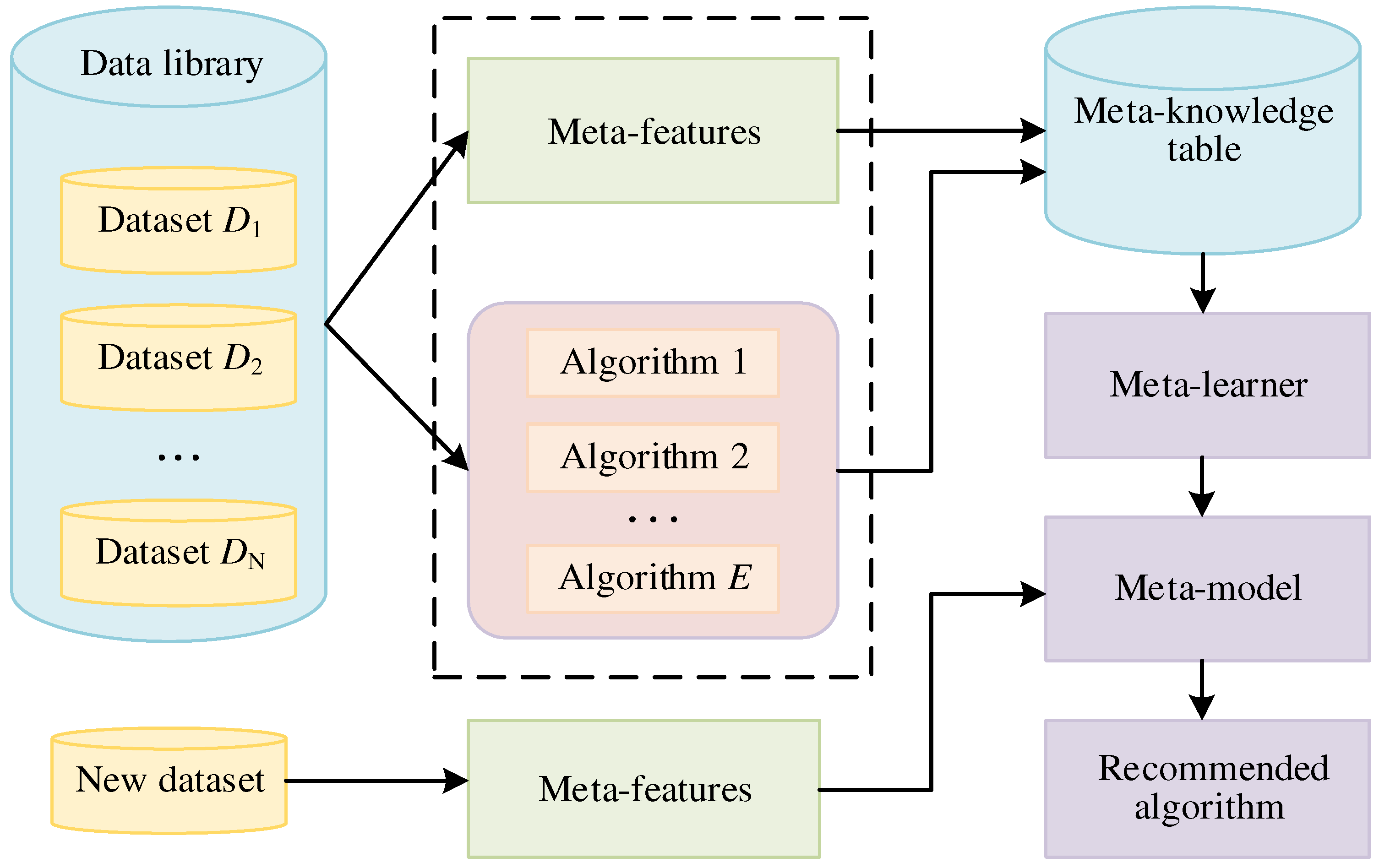
HEAs have excellent properties that are considerably affected by their phase structures [35]. The phases of HEAs include SS, IM, SS+IM, and AM. Some scholars have adopted the parameter method to determine the phase formation of HEAs in the materials field [5,11,12,13].

To date, the main parameters of HEAs include $\delta$, $\Delta H_{mix}$, $\mathsf{\Omega }$, $\Delta \chi$, and $\Delta S_{mix}$. The formulae of these parameters are shown in Equations (1)–(5) [11,12]:

$$\delta =\sqrt{{\displaystyle {\sum }_{i=1}^n{c}_i{(1-r_i/\overline{r})}_{}^2}}$$

(1)

where $\delta$ is the mean square deviation of atomic size of all elements in multi-principal alloy, c_i is the atomic percentage of the i-th element, r_i is the atomic radius of the i-th principal element, and $\overline{r}$ is the weighted average atomic radius of all principals, $\overline{r}={\displaystyle {\sum }_{i=1}^n{c}_i}{r}_i$.

$$\Delta H_{mix}={\displaystyle {\sum }_{i=1,i<j}^{n}4H_{ij}{c}_i}{c}_j$$

(2)

where $\Delta H_{mix}$ is the enthalpy of mixing; H_ij is the mixing enthalpy of i-th and j-th binary liquid alloy; and c_i and c_j are the atomic percentage of the i-th and j-th element, respectively.

$$\Delta S_{mix}=-R{\displaystyle {\sum }_{i=1}^n{c}_i\ln c_i}$$

(3)

where $\Delta S_{mix}$ is the entropy of mixing; c_i is the atomic percentage of the i-th element; and R is the gas constant, the value of which is 8.314 J·K⁻¹·mol⁻¹.

$$\mathsf{\Omega }=\frac{T_m\Delta S_{mix}}{|\Delta H_{mix}|}$$

(4)

where $\mathsf{\Omega }$ is the number of states of multi-principal element alloy system molecules; and T_m is the weighted average melting point for all elements, $T_m={\displaystyle {\sum }_{i=1}^n{c}_i}{T}_m^i$.

$$\Delta \chi ={\displaystyle {\sum }_{i=1}^n{c}_i({\chi }_i-\overline{\chi })}$$

(5)

where $\Delta \chi$ is the electronegativity difference of the HEA system, and $\overline{\chi }={\displaystyle {\sum }_{i=1}^n{c}_i}{\chi }_i$, ${\chi }_i$ is the electronegativity of constituent elements.

2.2. Meta-Learning

Meta-learning is utilized to solve the problem of algorithm selection [36,37]. The meta-learning method establishes the relationship between different datasets and the performance of algorithms to recommend the most appropriate algorithm. A schematic diagram of meta-learning is shown in Figure 1.

In Figure 1, the data library contains N datasets, including D₁, D₂, …, D_N. The selection of meta-features significantly affects the performance of meta-learning. The simple, statistical, and information theoretic meta-features can reflect the characteristic of several datasets [24,26,29,38]. In Figure 1, there are E candidate algorithms. The meta-knowledge table is constructed by meta-features and performance of candidate algorithms. The meta-learner is a very important part of meta-learning. The meta-learner is trained based on the meta-knowledge table, which takes the meta-features of datasets as input variables and yields the performance of algorithms as output variables. The KNN method is often used as a meta-learner in the literature [28,29]. The meta-model is a trained meta-learner that maps relationships between the meta-features of datasets and the performance of candidate algorithms. The algorithm steps for meta-learning are as follows:

Step 1: Compute the meta-features of each dataset.

Step 2: Train each algorithm on each dataset to evaluate its performance.

Step 3: Construct the meta-knowledge table with the meta-features of datasets and the performance of candidate algorithms.

Step 4: Train the meta-learner based on the meta-knowledge table to map the relationship between meta-features and performance of the candidate algorithms. The trained meta-learner is also called the meta-model.

Step 5: Compute the meta-features of the new dataset and predict the performance of candidate algorithms on the new dataset by the meta-model. Select the algorithm with the highest predictive performance as the recommended algorithm.

2.3. Shelly Nearest Neighbor

The SNN is a neighbor-instance selection method for classification and regression problems. Given an instance, its shelly nearest neighbors refer to the nearest neighbors that make up the shell to encapsulate the instance [39]. The SNN method considers its left and right nearest neighbors of each attribute in a given dataset [31]. The specific steps of the SNN algorithm are as follows [40].

Let $F=\left\{f_1,f_2,\dots ,f_R\right\}$ be the set of R class labels and $D=\{(x_1,y_1),(x_2,y_2),\dots ,(x_N,y_N)\}$ be the dataset consisting of N instances, where x_i is a vector of M attributes, and $y_i\subseteq F$ is the label of the i-th instance, x_i.

For the j-th attribute ($1\le j\le M$), the left nearest neighbor of a query instance, x_t, within D refers to the instances whose value on the j-th attribute is smaller than x_t but larger than the rest. The left nearest neighbor of a query instance, x_t, on the j-th attribute is defined as follows (Equation (6)):

$$x_t^{-}(D,j)=\{x_i\in D|x_{kj}\le x_{ij}\le x_{tj},1\le i,k\le N\}$$

(6)

where x_ij is the j-th attribute value of x_i. According to this definition, if x_tj was not the smallest one, x_t has at least one left nearest neighbor, $x_i\in D$, on the j-th attribute, such that $x_{ij}\le x_{tj}$, whereas $x_{kj}\le x_{ij}$ for the remaining instances, x_k, within D. Based on Equation (6), the left nearest neighbors of x_t over all attributes within D are represented as Equation (7):

$$x_t^{-}(D)={\cup }_{j=1..M}{x}_t^{-}(D,j)$$

(7)

In a similar way, the right nearest neighbors of x_t over all attributes within D are represented as Equation (8):

$$x_t^{+}(D)={\cup }_{j=1..M}{x}_t^{+}(D,j)$$

(8)

where $x_t^{+}(D,j)$ is the right nearest neighbors of x_t with respect to the j-th attribute, as shown in Equation (9):

$$x_t^{+}(D,j)=\{x_i\in D|x_{kj}\ge x_{ij}\ge x_{tj},1\le i,k\le N\}$$

(9)

The SNN of x_t within D refers to its left and right nearest neighbors, as shown in Equation (10):

$$SNN(x_t)=x_t^{+}(D)\cup x_t^{-}(D)$$

(10)

Generally speaking, there are about $2\times M$ shelly nearest neighbors for x_t if D has M attributes. For ease of understanding, the SNN of the query instance is shown in Figure 2.

Figure 2 shows an instances diagram of two-dimensional distribution. The red triangle is the query instance, marked as Query. The blue quadrangle is the neighbor instances of the query instance, which are selected by the SNN. x_t is the query instance. The right nearest neighbor set, $x_t^{+}(D,j)$, is composed of all instances in dataset D whose values are greater than or equal to x_tj. The left nearest neighbor set, $x_t^{-}(D,j)$, is composed of all instances in dataset D whose values are less than or equal to x_tj. The total dimension number is M = 2, where j = 1 represents the horizontal axis variable and j = 2 represents the vertical axis variable. x_t1 and x_t2 represents the horizontal and vertical axis value of the query instance, respectively.

The selection process of neighbor instances of x_t is as follows: First, the horizontal axis value and the vertical axis value of all instances in the dataset, D, are compared with x_t1 and x_t2, respectively. Secondly, if the value of the horizontal axis variable of the instances is greater or less than x_t1, these instances form the instance set $x_t^{+}(D,1)$ or $x_t^{-}(D,1)$. If the value of the vertical axis variable of the instances is greater or less than x_t2, these instances form the instance set $x_t^{+}(D,2)$ or $x_t^{-}(D,2)$. Thirdly, the left and right nearest neighbor of query instance x_t along the horizontal axis are x₁ and x₂, which are the maximum or minimum in $x_t^{-}(D,1)$ or $x_t^{+}(D,1)$. Fourthly, the instance with a maximum value in $x_t^{-}(D,2)$ is x₃, and the instance with a minimum value in $x_t^{+}(D,2)$ is the same instance, x₃. The left and right nearest neighbor of query instance x_t along the vertical axis is the same instance, x₃. Thus, the shelly nearest neighbor set of the query sample x_t instance includes instances x₁, x₂, and x₃.

2.4. Decremental Instance Selection for KNN Regression

Decremental instance selection for KNN regression was first proposed by Song [30]. DISKR is an effective instance selection algorithm for KNN regression that removes outliers and the samples with less effect in the training set for KNN.

The KNN regressor is learned by comparing the given test instances with the training set. Let $D=\{(x_1,y_1),(x_2,y_2),\dots ,(x_N,y_N)\}$ be the training set, where $x_i=(x_{i1},x_{i2},\dots ,x_{iM})$ is the i-th instance with M attributes, and y_i is the output of x_i. N is the number of instances. When a query instance, x_t, is given, the distance, d_i, between x_t and each instance, x_i, in D is calculated first, and then d_i is sorted by ascending order. The first k instances whose d_i ranks ahead are selected as k nearest neighbors of x_t, and the predicted output, $\widehat{y_t}$, of x_t is the average value of y_i of k nearest neighbors.

The specific steps of DISKR are as follows:

Input: Dataset $D=\{(x_1,y_1),(x_2,y_2),\dots ,(x_N,y_N)\}$, The parameter $\theta$.

Output: The subset $S\subseteq D$.

Step 1: Remove outliers. If $PD(x_i)=|y_i-\widehat{y_i}|>(1-\theta )y_i$, then the instance x_i is an outlier instance and removed; otherwise, it is not an outlier instance and is retained. y_i is the output of x_i; $\widehat{y_i}$ is the predicted output of x_i.

Step 2: Sort the remaining instances after removing outliers. Sort instances, x_i, by the absolute difference, $PD(x_i)=|y_i-\widehat{y_i}|$, in descending order.

Step 3: Delete instances with less effect on the KNN regressor. The effect of x_i could be estimated by the change in performance of KNN over D and $D-\left\{x_i\right\}$. The training error is used to approximately estimate the performance of KNN, which is expressed by the residual sum of squares (RSS).

$R_{bf}(x_i)$ is the RSS on the D. $R_{af}(x_i)$ is the RSS on the $D-\left\{x_i\right\}$, which represents the training set without x_i. $R_{bf}(x_i)$ and $R_{af}(x_i)$ are shown in Equations (11) and (12):

$$R_{bf}(x_i)={\displaystyle {\sum }_{x_j\in D-\left\{x_i\right\}}{(y_j-\widehat{y_j})}^2}$$

(11)

$$R_{af}(x_i)={\displaystyle {\sum }_{x_j\in D-\left\{x_i\right\}}{(y_j-\widehat{{y^{\prime }}_j})}^2}$$

(12)

where $\widehat{y_j}$ ($1\le j\le N,j\ne i$) and $\widehat{{y^{\prime }}_j}$ ($1\le j\le N,j\ne i$) are the predicted output of KNN based on D and $D-\left\{x_i\right\}$.

The effect of x_i on KNN is represented as Equation (13):

$$\nabla (x_i)=R_{af}(x_i)-R_{bf}(x_i)$$

(13)

After an instance, x_i, is removed, the following rule is adopted to avoid a significant negative change in the performance of the regressor, as shown in Equation (14):

$$\nabla (x_i)\le \theta R_{bf}(x_i)$$

(14)

where $\theta \in (0,1)$ is the significant coefficient.

Step 4: Output the subset S; the remaining samples in the subset S are more relative samples that remove outliers and points that have less effect on KNN.

3. Methodology

In this section, the phase prediction of high-entropy alloys (PPH) is proposed by integrating machine learning recommendation method and criterion to predict the phases of HEAs.

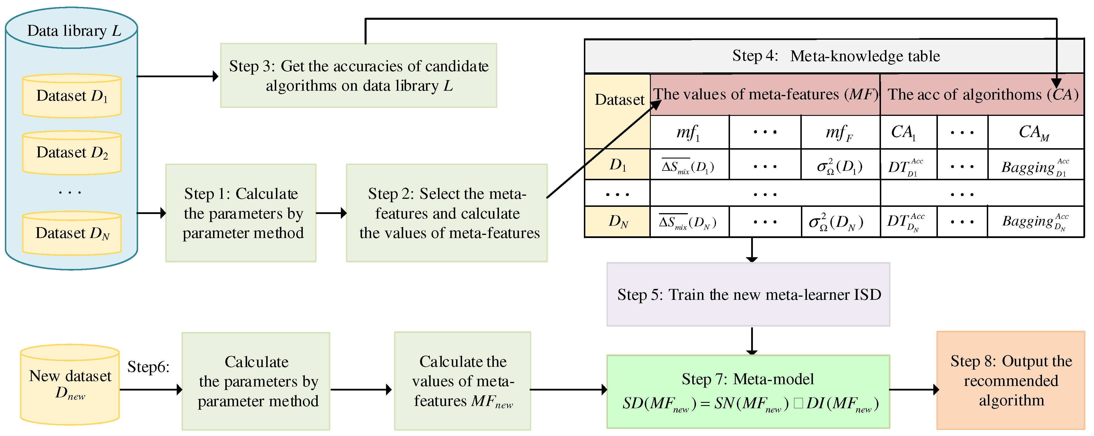
3.1. Machine Learning Recommendation Method

An MLRM based on improved meta-learning is proposed. The schematic diagram shown in Figure 3 illustrates MLRM, which can guide material designers to recommend an ideal algorithm.

As shown in Figure 3, the data library, $L=\{D_1,D_2,\dots ,D_N\}$, contains N datasets. D_i is the i-th dataset of L. The parameters $\Delta S_{mix}$, $\Delta H_{mix}$, $\delta$, Δχ, and $\mathsf{\Omega }$ of each sample in each dataset, D_i, are calculated by the parameter method [11,12]. The meta-features should reflect the characteristic of the datasets. The meta-feature set, $MF=\{m{f}_1,m{f}_2,\dots ,m{f}_F\}$, includes $\overline{\Delta S_{mix}}$, $\overline{\Delta H_{mix}}$, $\overline{\delta }$, $\overline{\Delta \chi }$, $\overline{\mathsf{\Omega }}$, ${\sigma }_{\Delta S_{mix}}^2$, ${\sigma }_{\Delta H_{mix}}^2$, ${\sigma }_{\delta }^2$, ${\sigma }_{\Delta \chi }^2$, and ${\sigma }_{\mathsf{\Omega }}^2$. $\overline{\Delta S_{mix}}$, $\overline{\Delta H_{mix}}$, $\overline{\delta }$, $\overline{\Delta \chi }$, and $\overline{\mathsf{\Omega }}$ are the mean value of $\Delta S_{mix}$, $\Delta H_{mix}$, $\delta$, $\Delta \chi$, and $\mathsf{\Omega }$, respectively; and ${\sigma }_{\Delta S_{mix}}^2$, ${\sigma }_{\Delta H_{mix}}^2$, ${\sigma }_{\delta }^2$, ${\sigma }_{\Delta \chi }^2$, and ${\sigma }_{\mathsf{\Omega }}^2$ are the variance of $\Delta S_{mix}$, $\Delta H_{mix}$, $\delta$, $\Delta \chi$, and $\mathsf{\Omega }$, respectively, in each dataset. The candidate algorithm set, $C=\{C_1,C_2,\dots ,C_M\}$, includes the decision tree (DT), KNN, SVM, random forest (RF), and bagging. The meta-knowledge table describes the relationship between the values of meta-features (MF) and the accuracy of candidate algorithms (CA).

The new meta-learner based on SNN and DISKR is proposed to improve the performance of meta-learning and is called improved SNN and DISKR (ISD). Therefore, an MLRM based on improved meta-learning is proposed. The meta-model is the trained meta-learner, ISD.

The steps of the MLRM are as follows:

Input: Data library $L=\{D_1,D_2,\dots ,D_N\}$, Candidate algorithm set $C=\{C_1,C_2,\dots ,C_M\}$, New dataset D_new.

Output: Recommendation algorithm.

Step 1: Compute the parameters $\Delta S_{mix}$, $\Delta H_{mix}$, $\delta$, $\Delta \chi$, and $\mathsf{\Omega }$ of each sample in each dataset, D_i, by Equations (1)–(5) in Section 2.1.

Step 2: Construct meta-features and calculate the values of meta-features: $\overline{\Delta S_{mix}}$, $\overline{\Delta H_{mix}}$, $\overline{\delta }$, $\overline{\Delta \chi }$, $\overline{\mathsf{\Omega }}$, ${\sigma }_{\Delta S_{mix}}^2$, ${\sigma }_{\Delta H_{mix}}^2$, ${\sigma }_{\delta }^2$, ${\sigma }_{\Delta \chi }^2$, and ${\sigma }_{\mathsf{\Omega }}^2$.

Step 3: Based on the values of meta-features and the real classification results on each dataset, train candidate algorithms DT, KNN, SVM, RF, and bagging in candidate algorithm set $C=\{C_1,C_2,\dots ,C_M\}$ to evaluate their accuracies.

Step 4: The meta-knowledge table is established based on meta-features of datasets and accuracies of candidate algorithms. The values of meta-features are used as the input variable (MF). The accuracies of candidate algorithms are used as the output variable (CA).

Step 5: Train the new meta-learner, ISD, based on the input variable, MF, and output variable, CA, in Step 4. Thus, obtain the trained meta-learner ISD, also known as the meta-model.

Step 6: Compute parameters of each sample in the new dataset, D_new, by the parameter method: $\Delta S_{mix}$, $\Delta H_{mix}$, $\delta$, $\Delta \chi$, and $\mathsf{\Omega }$. Compute the values of meta-features, MF_new, of the new dataset, D_new: $\overline{\Delta S_{mix}}$, $\overline{\Delta H_{mix}}$, $\overline{\delta }$, $\overline{\Delta \chi }$, $\overline{\mathsf{\Omega }}$, ${\sigma }_{\Delta S_{mix}}^2$, ${\sigma }_{\Delta H_{mix}}^2$, ${\sigma }_{\delta }^2$, ${\sigma }_{\Delta \chi }^2$, and ${\sigma }_{\mathsf{\Omega }}^2$.

Step 7: Input meta-features, MF_new, of the new dataset, D_new, to the meta-model. The realization process of the meta-model is as follows.

(1)

The nearest neighbor set, $SNN(M{F}_{new})$, for the meta-features, MF_new, of the new dataset, D_new, is obtained by SNN in Section 2.3 based on the meta-knowledge table.

(2)

The subset, S, is obtained by DISKR in Section 2.4, which is the remaining sample on the meta-knowledge table after removing outliers and points that have less effect on KNN. The nearest neighbor set, $DI(M{F}_{new})$, for the meta-features, MF_new, is obtained by the first k samples with the smallest distance in DISKR.

(3)

Obtain the nearest neighbor set, $SD(M{F}_{new})$, for the meta-features, MF_new, of the new dataset, D_new, by ISD. The nearest neighbor set, $SD(M{F}_{new})$, is shown as Equation (15):

$$SD(M{F}_{new})=SNN(M{F}_{new})\cap DI(M{F}_{new})$$

(15)

where the nearest neighbor set, $SD(M{F}_{new})$, is obtained by the intersection of $SNN(M{F}_{new})$ and $DI(M{F}_{new})$.

Step 8: Output the average accuracies of candidate algorithms by $SD(M{F}_{new})$. Select the algorithm with the highest average accuracy as the recommended algorithm.

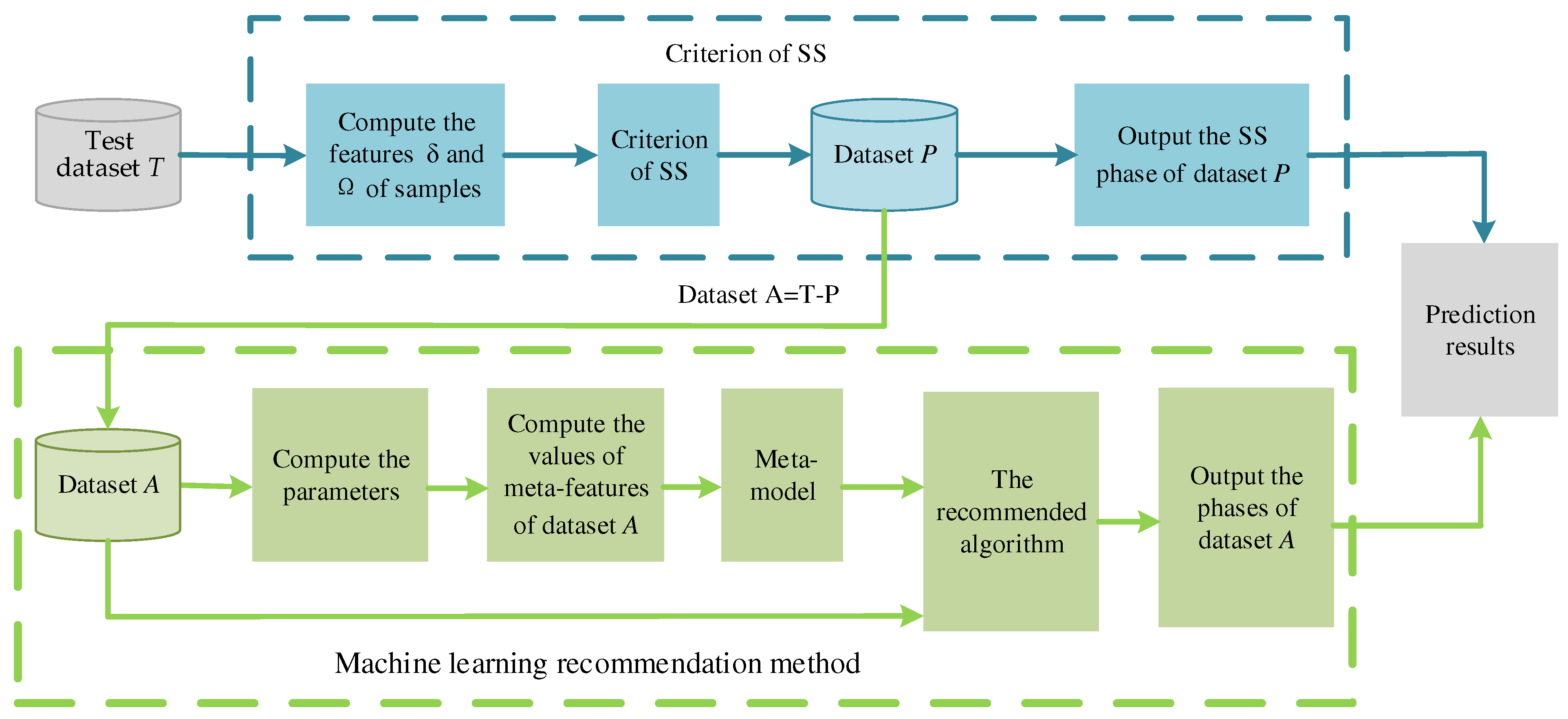
3.2. Phase Prediction of HEAs

The criterion of the SS phase has been verified by a large number of experiments in the material field. In the criterion of SS, if $\delta$ and $\mathsf{\Omega }$ fall within the range of $\delta \le 6.6\%$ and $\mathsf{\Omega }\ge 1.1$, the SS phase is easily formed [5,11,13]. The decision process of the criterion is easy to understand, saves computation time, and has strong interpretability and generalization. In this paper, the criterion of SS is integrated into the phase prediction of HEAs.

Combining the advantages of strong learning ability of MLRM and strong interpretability and generalization of the criterion of SS, the phase prediction of HEAs is proposed by integrating criterion and MLRM. The PPH is a serial model. First, the criterion of the SS phase is used to determine the phases of the test dataset, T. Secondly, when the remaining samples cannot be determined by the criterion of SS, the MLRM is adopted to recommend the appropriate ML algorithm for the remaining samples. Finally, the recommended algorithm is used to predict the phase of HEAs.

A schematic diagram of the PPH is shown in Figure 4.

In Figure 4, the blue frame is the criterion of SS, and the green frame is the MLRM. The specific details of the PPH are illustrated as follows:

Input: Test dataset $T=\{t_1,t_2,\dots t_N\}$.

Output: Phases of samples in T.

Step 1: Compute the features $\delta$ and $\mathsf{\Omega }$ of samples in test dataset T. Utilize the criterion of SS to judge the phase of samples. The dataset, $P=\{p_1,p_2,\dots ,p_J\}$, is composed of samples satisfying $\delta \le 6.6\%$ and $\mathsf{\Omega }\ge 1.1$. Output: the judgement results of samples in the dataset, P, are SS.

Step 2: In addition to the samples of dataset P, the remaining samples of the test dataset, T, constitute dataset $A=\{a_1,a_2,\dots ,a_Q\}$, that is, A = T − P. When the criterion of SS cannot judge the samples of dataset A, the machine learning recommendation method is adopted to predict phases of HEAs.

Step 3: For dataset A, compute the parameters of each sample in dataset A by Equations (1)–(5) in Section 2.1, and compute the values of meta-features of dataset A. Then, input the values of meta-features into the meta-model.

Step4: Predict the accuracies of the candidate algorithms by meta-model, and select an ideal algorithm as the recommended algorithm in dataset A.

Step5: The recommended algorithm is used to predict the phase of dataset A.

Step6: Output the phases of test dataset T, combining results of dataset P and dataset A.

4. Results and Discussions

In order to verify the effectiveness of the proposed PPH, numerous experiments are carried out. The accuracy of the proposed method is compared with several traditional ML algorithms, including DT, KNN, SVM, RF, and bagging [41,42,43]. In this paper, the parameters of the algorithms in this experiment are introduced. In DT, the hyperparameter ‘maximum depth’ is set to ‘25’. The hyperparameter ‘k’ of KNN is set to ‘5’. The support vector classification (SVC) method is used in SVM. In bagging, the hyperparameter ‘number of weak learners’ is set to ‘11’. In ISDISKR, the hyperparameter ‘$\theta$’ is set as ‘0.05’. The other parameters of all ML algorithms above are set as default.

The experiments are carried out by the sklearn library of Python (version 3.7.4). Python was created by Guido van Rossum in Amsterdam, the Netherlands. The hardware device is a laptop, and the brand of the computer is Lenovo. The CPU is an Intel(R) Core(M) I7-8700 CPU @ 3.20 GHz 3.19 GHz, the RAM is 16.0 GB, the manufacturer is Lenovo Group Limited, and the location is Beijing, China.

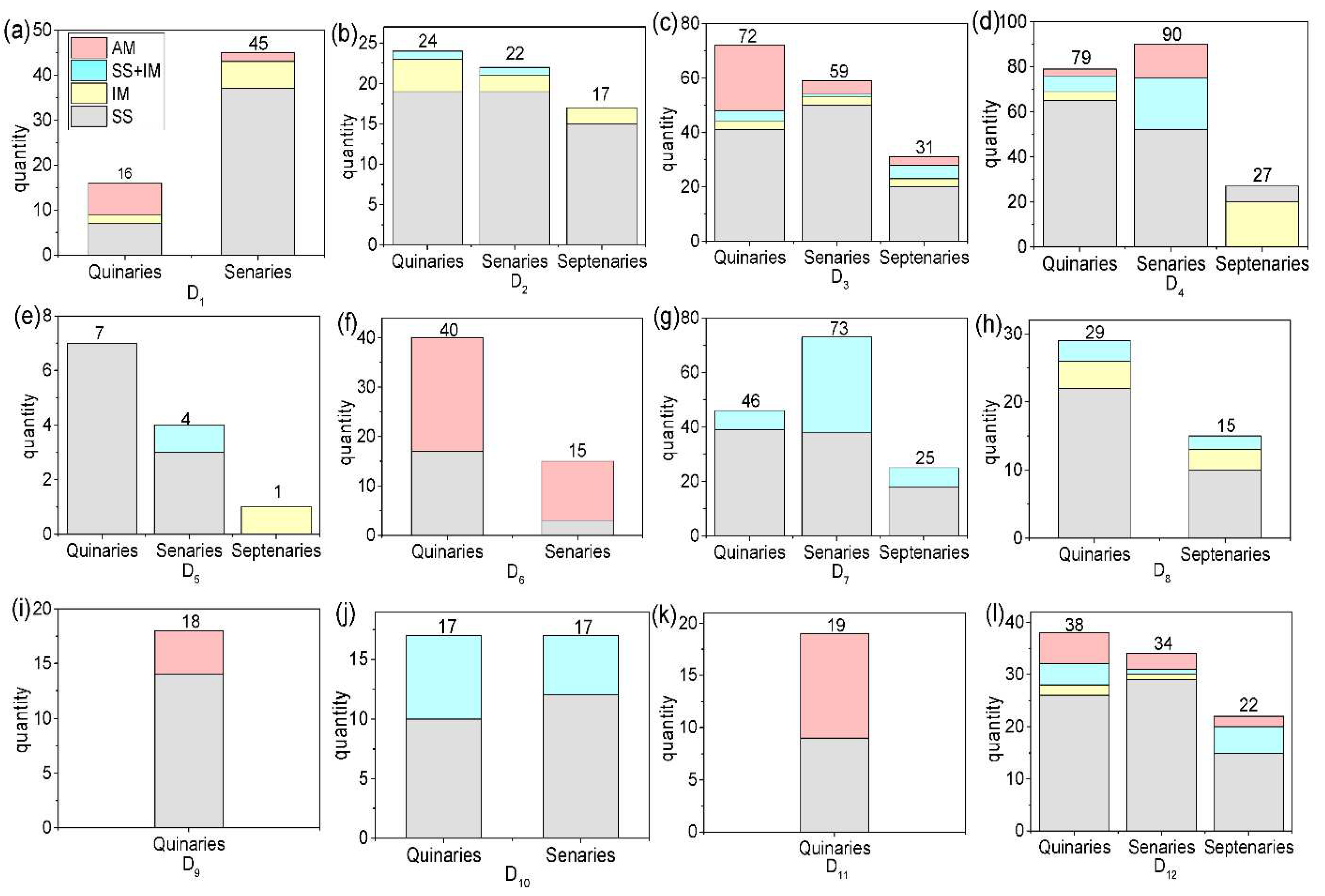
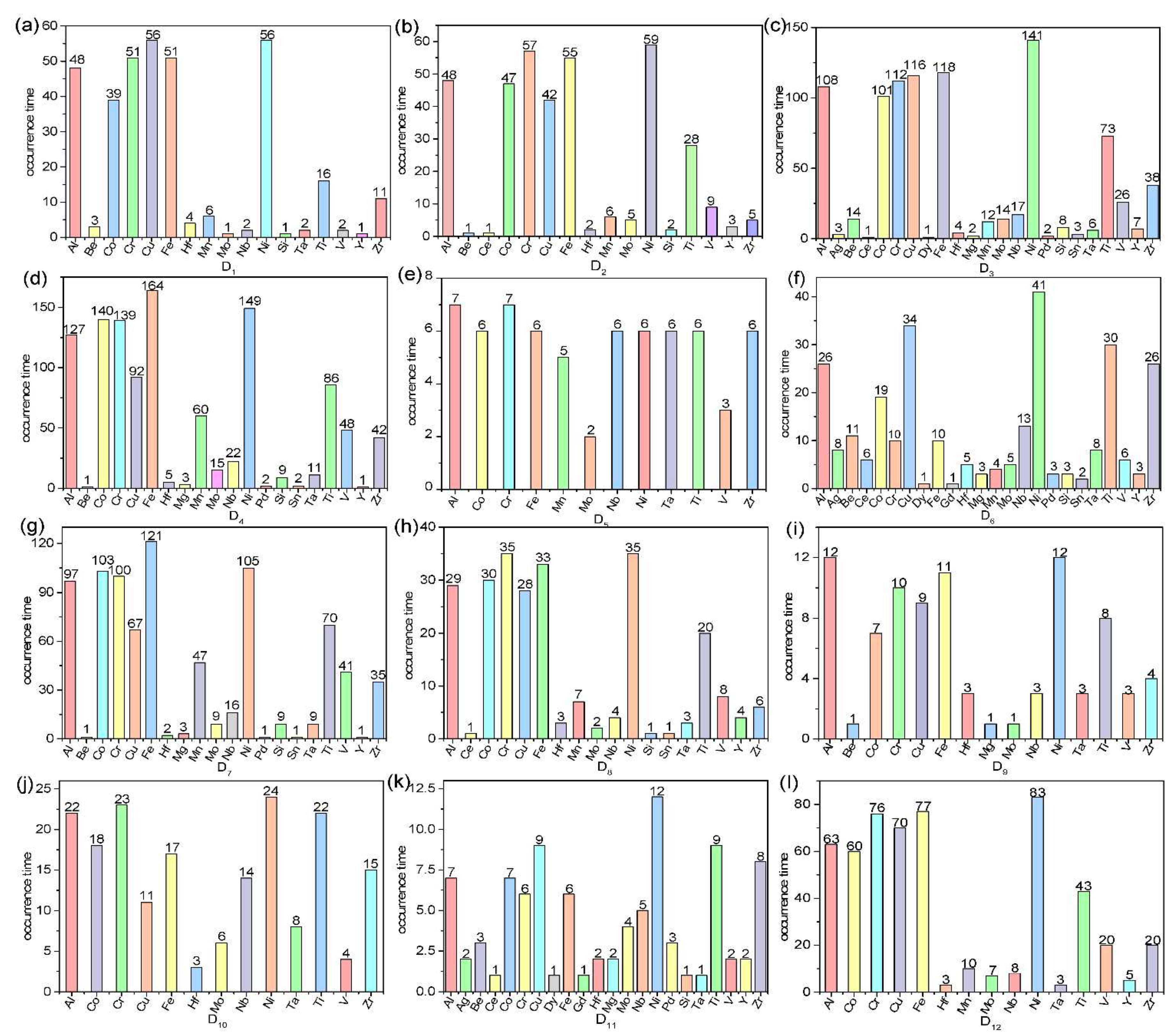
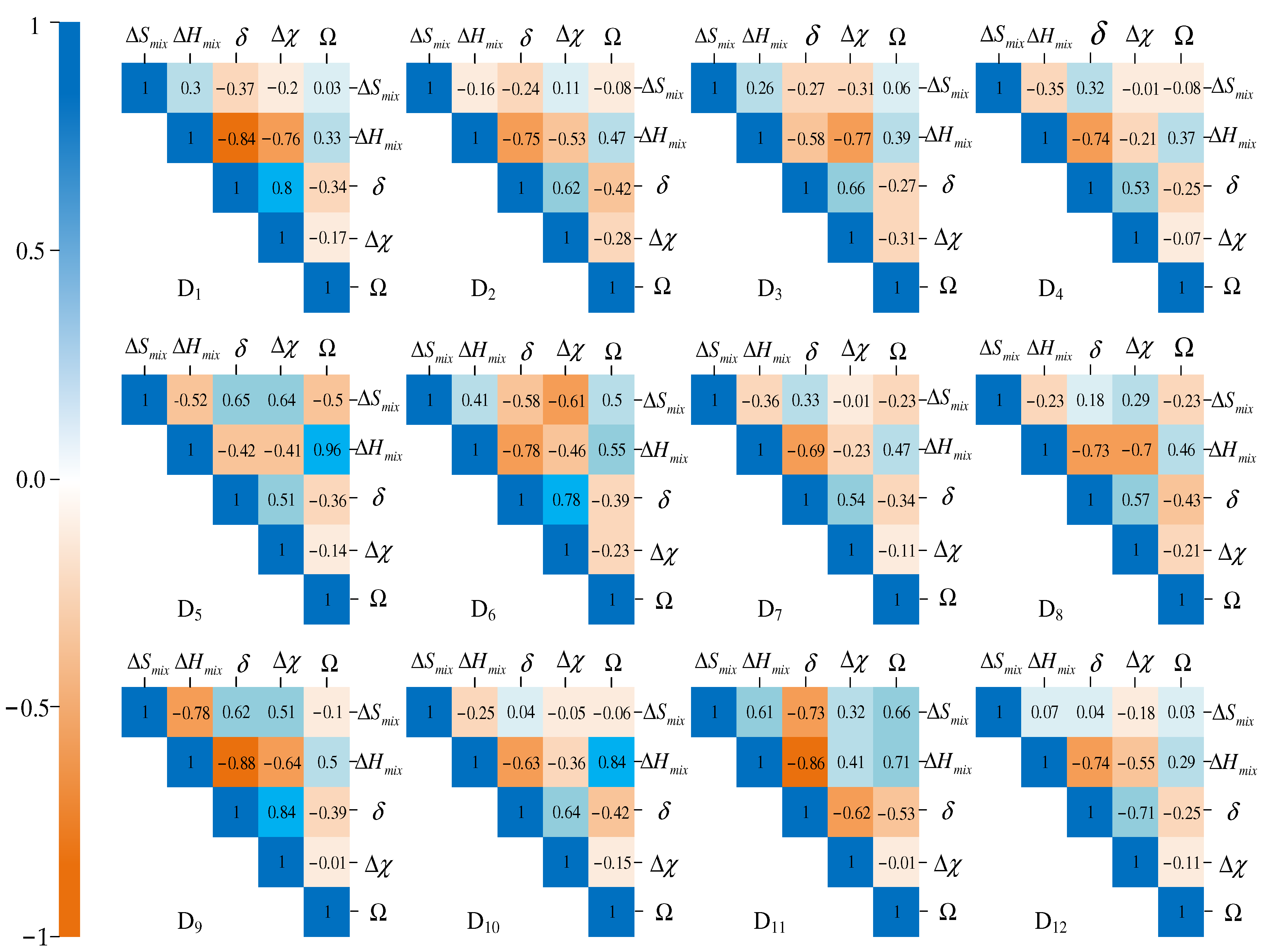
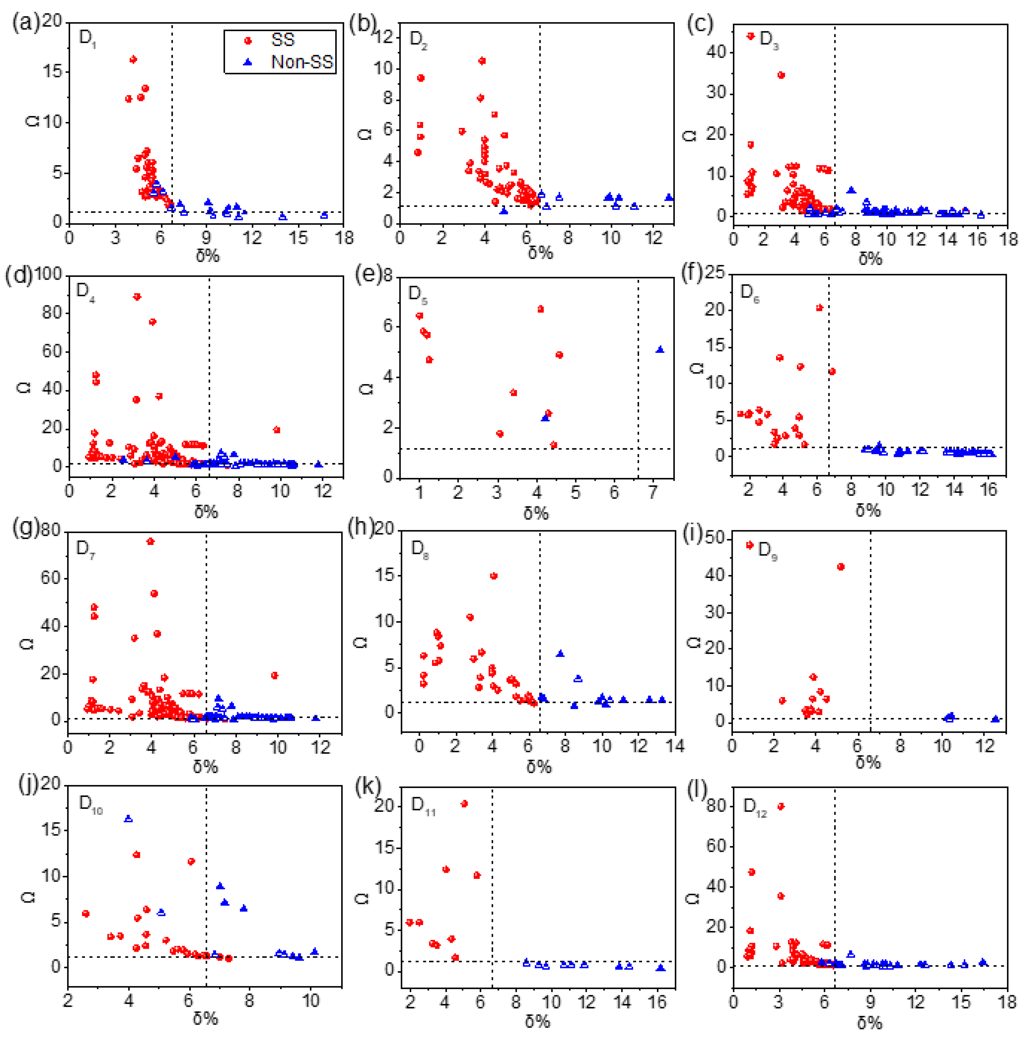
4.1. Overview of Experimental Datasets

In our study, the 12 HEAs datasets were collected from several papers [4,6,7,10,14,44,45,46,47,48,49]. For convenience, the 12 datasets are sequentially marked by D₁, D₂, D₃, D₄, D₅, D₆, D₇, D₈, D₉, D₁₀, D₁₁, and D₁₂. The 12 datasets contain 902 samples, including 405 quinary HEAs, 359 senary HEAs, and 138 septenary HEAs. The phases of 902 samples include SS, IM, SS+IM, and AM. The quantity of SS, IM, SS+IM, and AM of the quinaries, senaries, and septenaries in 12 datasets is shown in Figure 5. As shown in Figure 5, the number of SS is the largest, and the number of IM is the least among the 12 datasets. Figure 5 shows that each dataset contains different quantities of quinaries, senaries, and septenaries.

The 12 datasets include 24 elements, which contain Al, Ag, Be, Ce, Co, Cr, Cu, Dy, Fe, Gd, Hf, Mg, Mn, Mo, Nb, Ni, Pd, Si, Sn, Ta, Ti, V, Y, and Zr. The occurrence time of each element in each dataset is shown in Figure 6. As shown in Figure 6, the occurrence time of different elements varies. The elements Al, Co, Cr, Cu, Fe, Ni, and Ti appear more frequently, and the element Gd appears only once in 12 datasets.

The maximum and minimum values of the five input parameters, $\Delta S_{mix}$, $\Delta H_{mix}$, $\delta$, $\Delta \chi$, and $\mathsf{\Omega }$, are shown in

Table 1. Maximum values and minimum values of the five parameters.

Number	Parameter	Maximum Value	Minimum Value	Parameter Description
1	$\Delta S_{mix}$	16.18	7.78	thermodynamic parameter
2	$\Delta H_{mix}$	17.12	−48.64	chemical parameter
3	$\delta$	35.30	0.21	electronic parameter
4	$\Delta \chi$	23.10	0.04	electronic parameter
5	$\mathsf{\Omega }$	283.50	0.37	chemical thermodynamic parameter

.

A snapshot of part of the samples in the HEA dataset according to the Pandas data frame format is shown as

Table 2. Pandas snapshot of the first six samples.

Number	HEAs	$\mathbf{\Delta }{\mathit{S}}_{\mathit{m}\mathit{i}\mathit{x}}$	$\mathbf{\Delta }{\mathit{H}}_{\mathit{m}\mathit{i}\mathit{x}}$	$\mathbf{\delta }(\mathbf{\%})$	$\mathbf{\Delta }\mathit{\chi }$	$\mathsf{\Omega }$	Phase
0	AlCr0.5NbTiV	13.150000	−15.410000	5.230000	0.037647	1.680000	SS
1	Mg65Cu15Ag5Pd5Gd10	9.100000	−13.240000	9.360000	0.298062	0.770000	AM
2	AlCoCrFeNiSi0.6	14.778118	−22.755102	5.877203	0.120010	1.090691	SS+IM
3	CoFeMnTiVZr0.4	14.585020	−16.049383	8.088626	0.165697	1.692345	IM
4	Ti0.2CoCrFeNiCuAl0.5	15.445251	−4.148969	0.210000	0.118750	6.318158	SS
5	Al0.5CoCrCuFeNiTi0.8	15.995280	−10.100000	5.800000	0.137280	2.725683	SS+IM

. In Table 2, the first column is the number of HEAs, and the second column provides the names of the HEAs. The columns ranging from three to seven are the parameters of HEAs, i.e., $\delta$, $\Delta H_{mix}$, $\mathsf{\Omega }$, $\Delta \chi$, and $\Delta S_{mix}$. The final column is the phases of HEAs. Table 2 shows a snapshot of the first six samples taken from all HEAs.

The correlation between any two parameters in Table 2 plays an important role in phase prediction of HEAs, so the Pearson correlation coefficient, C_ab, is selected to describe the correlations of HEA parameters, as shown in Equation (16) [14]:

$$C_{ab}=\frac{1}{n-1}\frac{{\displaystyle {\sum }_{i=1}^n(a_i-\overline{a})(b_i-\overline{b})}}{s_a{s}_b}$$

(16)

where a_i and b_i are the sample values of parameters a and b, respectively; $\overline{a}$ and $\overline{b}$ are the mean values of parameters a and b, respectively; s_a and s_b are the standard deviation of parameters a and b, respectively; and n is the number of samples. If $C_{ab}=1$ or $C_{ab}=-1$, the parameters a and b are almost completely relevant or completely irrelevant, respectively. The correlation among the 5 parameters of 12 datasets is shown in Figure 7.

In Figure 7, the values of the correlation coefficient between the two corresponding parameters is shown in every grid. Color intensity is proportional to the correlation coefficients. In the left side of the correlogram, the legend color shows the relationship between the correlation coefficients and the corresponding color. The darker the blue color, the higher the correlation; the darker the orange color, the lower the correlation. The range of C_ab in 12 datasets is between−0.88 and 0.96. Among them, ∆H_mix and $\mathsf{\Omega }$ in D₅ have the highest correlation.

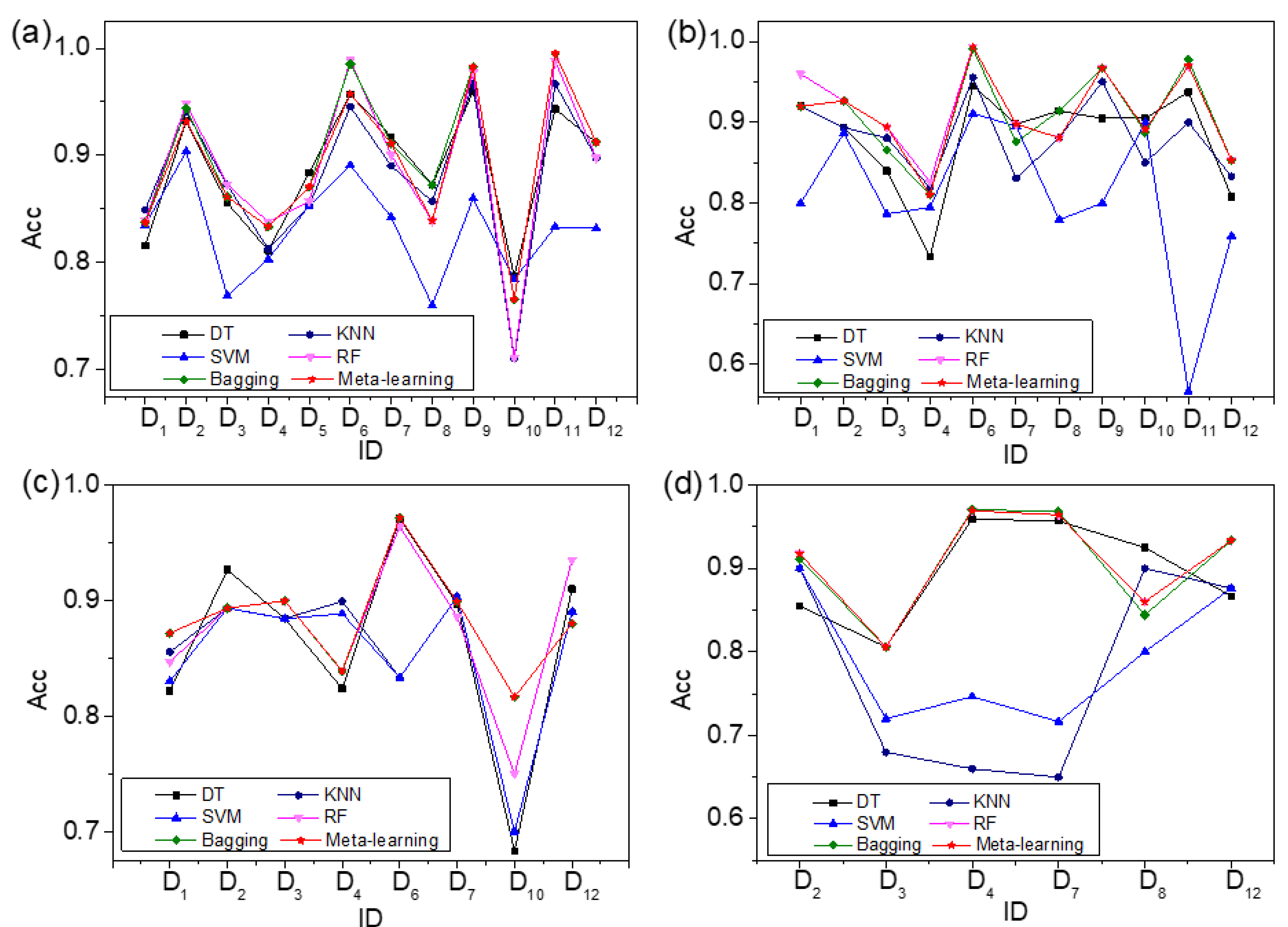
4.2. Comparison between Meta-Learning and Traditional ML Algorithms

The meta-learning based on meta-knowledge table can recommend an ideal algorithm for material designers so as to predict the phases of HEAs. In order to validate the performance of meta-learning, the experimental results of meta-learning are compared with the DT, KNN, SVM, RF, and bagging [41,42,43]. The fivefold cross-validation method is also carried out 20 times to avoid the overfitting problem of ML algorithms [50]. The comparison experimental results between meta-learning and traditional ML algorithms for all, quinaries, senaries, and septenaries are shown in Figure 8. In Figure 8, the experimental results of all, quinaries, senaries, and septenaries between meta-learning and other traditional ML algorithms are shown in (a), (b), (c), and (d), respectively. In Figure 8a, “all” represents samples containing quinaries, senaries, and septenaries. The horizontal axis represents the ID of these datasets, and the vertical axis represents the accuracies of meta-learning and traditional ML algorithms. The red line with pentagonal stars represents the accuracy of algorithms recommended by meta-learning. The black line with squares shows the accuracy of DT. The navy line with circles shows the accuracy of KNN. The blue line with upward triangles represents the accuracy of SVM. The pink line with downward triangles shows the accuracy of RF, and the olive line with diamonds represents the accuracy of bagging. Based on the results presented in Figure 8, the algorithm with the highest accuracy can be recommended by meta-learning on some datasets.

In order to facilitate the reader’s observation, the results of all, quinaries, senaries, and septenaries are shown in

Table 3. Accuracy comparison between meta-learning and traditional ML algorithms in all.

ID	DT	KNN	SVM	RF	Bagging	Meta-Learning
D1	0.816 ± 0.012	0.849 ± 0.008	0.835 ± 0.007	0.839 ± 0.010	0.837 ± 0.005	0.837 ± 0.005
D2	0.932 ± 0.003	0.941 ± 0.022	0.904 ± 0.009	0.949 ± 0.013	0.944 ± 0.020	0.932 ± 0.003
D3	0.856 ± 0.008	0.873 ± 0.019	0.769 ± 0.013	0.873 ± 0.003	0.861 ± 0.002	0.861 ± 0.002
D4	0.811 ± 0.005	0.813 ± 0.012	0.803 ± 0.017	0.838 ± 0.009	0.833 ± 0.014	0.833 ± 0.014
D5	0.884 ± 0.030	0.853 ± 0.016	0.853 ± 0.011	0.857 ± 0.012	0.871 ± 0.030	0.871 ± 0.030
D6	0.957 ± 0.009	0.945 ± 0.004	0.891 ± 0.007	0.989 ± 0.007	0.985 ± 0.008	0.957 ± 0.009
D7	0.918 ± 0.010	0.890 ± 0.027	0.842 ± 0.005	0.900 ± 0.008	0.911 ± 0.009	0.911 ± 0.009
D8	0.873 ± 0.025	0.857 ± 0.017	0.760 ± 0.023	0.839 ± 0.011	0.872 ± 0.006	0.839 ± 0.011
D9	0.960 ± 0.003	0.967 ± 0.006	0.860 ± 0.009	0.978 ± 0.010	0.983 ± 0.010	0.983 ± 0.010
D10	0.787 ± 0.009	0.711 ± 0.019	0.784 ± 0.010	0.712 ± 0.012	0.766 ± 0.026	0.766 ± 0.026
D11	0.943 ± 0.006	0.967 ± 0.016	0.833 ± 0.022	0.988 ± 0.002	0.995 ± 0.002	0.995 ± 0.002
D12	0.912 ± 0.004	0.898 ± 0.012	0.832 ± 0.009	0.898 ± 0.015	0.912 ± 0.003	0.912 ± 0.003

,

Table 4. Accuracy comparison between meta-learning and traditional ML algorithms in quinaries.

ID	DT	KNN	SVM	RF	Bagging	Meta-Learning
D1	0.920 ± 0.005	0.920 ± 0.003	0.800 ± 0.002	0.960 ± 0.027	0.920 ± 0.002	0.920 ± 0.002
D2	0.893 ± 0.015	0.893 ± 0.012	0.887 ± 0.009	0.927 ± 0.005	0.927 ± 0.004	0.927 ± 0.004
D3	0.840 ± 0.005	0.881 ± 0.015	0.786 ± 0.017	0.894 ± 0.010	0.866 ± 0.010	0.894 ± 0.010
D4	0.733 ± 0.034	0.819 ± 0.011	0.795 ± 0.035	0.826 ± 0.034	0.810 ± 0.008	0.810 ± 0.008
D6	0.945 ± 0.025	0.956 ± 0.005	0.911 ± 0.005	0.994 ± 0.002	0.991 ± 0.001	0.994 ± 0.002
D7	0.898 ± 0.007	0.831 ± 0.004	0.895 ± 0.003	0.898 ± 0.005	0.876 ± 0.002	0.898 ± 0.005
D8	0.914 ± 0.004	0.881 ± 0.007	0.779 ± 0.016	0.881 ± 0.003	0.914 ± 0.006	0.881 ± 0.003
D9	0.905 ± 0.027	0.950 ± 0.011	0.800 ± 0.022	0.968 ± 0.006	0.968 ± 0.012	0.968 ± 0.006
D10	0.905 ± 0.004	0.850 ± 0.008	0.900 ± 0.003	0.891 ± 0.027	0.888 ± 0.007	0.891 ± 0.027
D11	0.938 ± 0.006	0.900 ± 0.024	0.567 ± 0.027	0.970 ± 0.009	0.978 ± 0.005	0.970 ± 0.009
D12	0.808 ± 0.025	0.833 ± 0.023	0.759 ± 0.029	0.853 ± 0.022	0.853 ± 0.033	0.853 ± 0.022

,

Table 5. Accuracy comparison between meta-learning and traditional ML algorithms in senaries.

ID	DT	KNN	SVM	RF	Bagging	Meta-Learning
D1	0.822 ± 0.015	0.855 ± 0.008	0.830 ± 0.014	0.847 ± 0.007	0.872 ± 0.006	0.872 ± 0.006
D2	0.927 ± 0.009	0.893 ± 0.013	0.893 ± 0.009	0.893 ± 0.020	0.893 ± 0.006	0.893 ± 0.006
D3	0.884 ± 0.008	0.884 ± 0.011	0.884 ± 0.018	0.900 ± 0.014	0.900 ± 0.013	0.900 ± 0.013
D4	0.824 ± 0.012	0.899 ± 0.017	0.889 ± 0.005	0.839 ± 0.010	0.838 ± 0.017	0.839 ± 0.010
D6	0.971 ± 0.010	0.833 ± 0.009	0.833 ± 0.011	0.964 ± 0.017	0.972 ± 0.012	0.972 ± 0.012
D7	0.897 ± 0.007	0.903 ± 0.002	0.903 ± 0.013	0.886 ± 0.008	0.899 ± 0.008	0.899 ± 0.008
D10	0.683 ± 0.023	0.700 ± 0.036	0.700 ± 0.010	0.750 ± 0.032	0.817 ± 0.006	0.817 ± 0.006
D12	0.910 ± 0.020	0.890 ± 0.007	0.890 ± 0.009	0.935 ± 0.005	0.880 ± 0.027	0.880 ± 0.027

and

Table 6. Accuracy comparison between meta-learning and traditional ML algorithms in septenaries.

ID	DT	KNN	SVM	RF	Bagging	Meta-Learning
D2	0.855 ± 0.031	0.900 ± 0.005	0.900 ± 0.007	0.918 ± 0.022	0.911 ± 0.013	0.918 ± 0.022
D3	0.806 ± 0.016	0.680 ± 0.008	0.720 ± 0.005	0.806 ± 0.007	0.806 ± 0.011	0.806 ± 0.007
D4	0.959 ± 0.009	0.660 ± 0.028	0.747 ± 0.012	0.969 ± 0.013	0.970 ± 0.005	0.969 ± 0.013
D7	0.957 ± 0.015	0.650 ± 0.019	0.717 ± 0.019	0.964 ± 0.009	0.968 ± 0.018	0.964 ± 0.009
D8	0.925 ± 0.033	0.900 ± 0.023	0.800 ± 0.035	0.860 ± 0.018	0.844 ± 0.017	0.860 ± 0.018
D12	0.867 ± 0.027	0.876 ± 0.034	0.876 ± 0.031	0.933 ± 0.022	0.933 ± 0.033	0.933 ± 0.022

. The bold part of the tables is the algorithm with the highest accuracy on the corresponding dataset.

In Table 3, the first column is the ID of 12 datasets, and the second column to the seventh column are the accuracies of DT, KNN, SVM, RF, bagging, and meta-learning, respectively. As shown in Table 3, meta-learning recommends the algorithm with the highest accuracy; in D₉, D₁₁, and D₁₂, the algorithms with the highest accuracy are bagging, bagging, and bagging, and the accuracies are 0.983, 0.995, and 0.912, respectively, for all. In D₄, D₅, and D₇, although meta-learning does not recommend the highest-accuracy algorithm, it recommends the algorithm with the second highest accuracy; the algorithms with the second highest accuracy are bagging, bagging, and bagging, and the accuracies are 0.833, 0.871, 0.911, respectively, for all.

It can be seen from Table 4 that meta-learning recommends the algorithm with the highest accuracy in D₂, D₃, D₆, D₇, D₉, and D₁₂, and the accuracies are 0.927, 0.894, 0.994, 0.898, 0.968, 0.853, respectively, for quinaries. Meta-learning recommends the algorithm with the second highest accuracy in D₁ and D₁₁; the algorithms with the second highest accuracy are bagging and RF in D₁ and D₁₁, respectively.

As shown in Table 5, meta-learning recommends the algorithm with the highest accuracy in D₁, D₃, D₆, and D₁₀ for senaries, and the accuracies are 0.872, 0.900, 0.972, 0.817, respectively. Meta-learning recommends the algorithm with the second highest accuracy in D₂ for senaries; the algorithm with the second highest accuracy is bagging in D₂.

In Table 6, the algorithm with the highest accuracy is recommended by meta-learning in D₂, D₃, and D₁₂ for septenaries; the algorithms with the highest accuracy are RF, RF, and RF in D₂, D₃, and D₁₂, respectively. Meta-learning recommends the algorithm with the second highest accuracy in D₄ and D₇ for septenaries; the accuracies are 0.969 and 0.964, respectively.

Meta-learning recommends the algorithm with the high highest accuracy in some datasets. The reason should be that meta-learning can mine the relationship between mathematical statistical characteristics of HEA datasets and the performance of algorithms. The mathematical statistical characteristics of datasets include the mean value and variance of these parameters presented in Section 2.1. It is similarly reported in the literature in other fields meta-learning can recommend the desirable algorithm in most cases [24,27]. The experimental results also show that RF and bagging have higher accuracies than DT, KNN, and SVM [41,42,43]. The reason could be that RF and bagging are both ensemble algorithms, which are composed of multiple classifiers and integrate all the classification results.

However, meta-learning cannot recommend the algorithm with the highest accuracy in some datasets. The reasons could be as follows: firstly, the meta-learner is the crucial part in meta-learning method, and the meta-learner of meta-learning is KNN. The performance of KNN is not ideal in ML algorithms. Secondly, the KNN does not fully consider the information of the left and right nearest neighbors of every sample by every attribute. Finally, the meta-learner, KNN, does not consider how to exclude the noise samples and make up for missing information, which influences the decision result of different algorithms. If the performance of the meta-learner can be improved, the recommendation of meta-learning will be more accurate.

4.3. Comparison between MLRM and Meta-Learning

To alleviate the problem presented in Section 4.2, a novel MLRM method is proposed based on improved meta-learning. In order to validate the performance of MLRM, a comparison between MLRM and meta-learning is shown in Figure 9. In Figure 9, the accuracies of MLRM and meta-learning of all, quinaries, senaries, and septenaries are shown in (a), (b), (c), and (d), respectively. The horizontal axis is the ID of these datasets, and the vertical axis is the accuracy. The red line with circles shows the accuracy of algorithms recommended by MLRM. The black line with squares represents the accuracy of algorithms recommended by meta-learning. It can be seen from Figure 9 that all experimental results of MLRM are better than those of meta-learning.

In order to facilitate the reader’s observation, the rankings of algorithms recommended by meta-learning and MLRM, as wells real rankings are listed in

Table 7. Recommendation results between MLRM and meta-learning in all.

ID	Meta-Learning	MLRM	TRUE
D1	Bagging, KNN	KNN, RF	KNN, RF
D2	DT, Bagging	RF, Bagging	RF, Bagging
D3	Bagging, RF	RF, Bagging	RF, KNN
D4	Bagging, DT	RF, Bagging	RF, Bagging
D5	Bagging, RF	DT, Bagging	DT, Bagging
D6	DT, Bagging	RF, Bagging	RF, Bagging
D7	Bagging, RF	DT, Bagging	DT, Bagging
D8	RF, Bagging	DT, Bagging	DT, Bagging
D9	Bagging, DT	Bagging, RF	Bagging, RF
D10	Bagging, RF	DT, Bagging	DT, SVM
D11	Bagging, RF	Bagging, RF	Bagging, RF
D12	Bagging, RF	Bagging, RF	Bagging, DT

,

Table 8. Recommendation results between MLRM and meta-learning in quinaries.

ID	Meta-Learning	MLRM	TRUE
D1	Bagging, RF	RF, Bagging	RF, Bagging
D2	Bagging, RF	Bagging, RF	Bagging, RF
D3	RF, Bagging	RF, Bagging	RF, KNN
D4	Bagging, RF	RF, Bagging	RF, KNN
D6	RF, Bagging	RF, Bagging	RF, Bagging
D7	RF, Bagging	RF, Bagging	RF, DT
D8	RF, Bagging	DT, Bagging	DT, Bagging
D9	RF, Bagging	RF, Bagging	RF, Bagging
D10	RF, Bagging	DT, RF	DT, SVM
D11	RF, Bagging	Bagging, RF	Bagging, RF
D12	RF, Bagging	RF, Bagging	RF, Bagging

,

Table 9. Recommendation results between MLRM and meta-learning in senaries.

ID	Meta-Learning	MLRM	TRUE
D1	Bagging, RF	Bagging, KNN	Bagging, KNN
D2	Bagging, RF	DT, Bagging	DT, Bagging
D3	Bagging, RF	Bagging, RF	Bagging, RF
D4	RF, Bagging	KNN, SVM	KNN, SVM
D6	Bagging, RF	Bagging, RF	Bagging, DT
D7	Bagging RF	KNN, SVM	KNN, SVM
D10	Bagging, DT	Bagging, RF	Bagging, RF
D12	Bagging RF	RF, DT	RF, DT

and

Table 10. Recommendation results between MLRM and meta-learning in septenaries.

ID	Meta-Learning	MLRM	TRUE
D2	RF, Bagging	RF, Bagging	RF, Bagging
D3	RF, Bagging	RF, Bagging	RF, Bagging
D4	RF, Bagging	Bagging, RF	Bagging, RF
D7	RF, Bagging	Bagging, RF	Bagging, RF
D8	RF, Bagging	DT, RF	DT, KNN
D12	RF, DT	RF, Bagging	RF, Bagging

. The accuracies of the optimal algorithms recommended by meta-learning and MLRM, as well as the accuracies of real optimal algorithms are listed in

Table 11. Accuracy comparison between MLRM and meta-learning in all.

ID	Meta-Learning	MLRM	TRUE
D1	0.837 ± 0.005	0.849 ± 0.008	0.849 ± 0.008
D2	0.932 ± 0.003	0.949 ± 0.013	0.949 ± 0.013
D3	0.861 ± 0.002	0.873 ± 0.003	0.873 ± 0.003
D4	0.833 ± 0.014	0.838 ± 0.009	0.838 ± 0.009
D5	0.871 ± 0.030	0.884 ± 0.030	0.884 ± 0.030
D6	0.957 ± 0.009	0.989 ± 0.007	0.989 ± 0.007
D7	0.911 ± 0.009	0.918 ± 0.010	0.918 ± 0.010
D8	0.839 ± 0.011	0.873 ± 0.025	0.873 ± 0.025
D9	0.983 ± 0.010	0.983 ± 0.010	0.983 ± 0.010
D10	0.766 ± 0.026	0.787 ± 0.009	0.787 ± 0.009
D11	0.995 ± 0.002	0.995 ± 0.002	0.995 ± 0.002
D12	0.912 ± 0.003	0.912 ± 0.003	0.912 ± 0.003

,

Table 12. Accuracy comparison between MLRM and meta-learning in quinaries.

ID	Meta-Learning	MLRM	TRUE
D1	0.920 ± 0.002	0.960 ± 0.027	0.960 ± 0.027
D2	0.927 ± 0.004	0.927 ± 0.004	0.927 ± 0.004
D3	0.894 ± 0.010	0.894 ± 0.010	0.894 ± 0.010
D4	0.810 ± 0.008	0.826 ± 0.034	0.826 ± 0.034
D6	0.994 ± 0.002	0.994 ± 0.002	0.994 ± 0.002
D7	0.898 ± 0.005	0.898 ± 0.005	0.898 ± 0.005
D8	0.881 ± 0.003	0.914 ± 0.004	0.914 ± 0.004
D9	0.968 ± 0.006	0.968 ± 0.006	0.968 ± 0.006
D10	0.891 ± 0.027	0.905 ± 0.004	0.905 ± 0.004
D11	0.970 ± 0.009	0.978 ± 0.005	0.978 ± 0.005
D12	0.853 ± 0.022	0.853 ± 0.022	0.853 ± 0.022

,

Table 13. Accuracy comparison between MLRM and meta-learning in senaries.

ID	Meta-Learning	MLRM	TRUE
D1	0.872 ± 0.006	0.872 ± 0.006	0.872 ± 0.006
D2	0.893 ± 0.006	0.927 ± 0.009	0.927 ± 0.009
D3	0.900 ± 0.013	0.900 ± 0.013	0.900 ± 0.013
D4	0.839 ± 0.010	0.899 ± 0.017	0.899 ± 0.017
D6	0.972 ± 0.012	0.972 ± 0.012	0.972 ± 0.012
D7	0.899 ± 0.008	0.903 ± 0.002	0.903 ± 0.002
D10	0.817 ± 0.006	0.817 ± 0.006	0.817 ± 0.006
D12	0.880 ± 0.027	0.935 ± 0.005	0.935 ± 0.005

and

Table 14. Accuracy comparison between MLRM and meta-learning in septenaries.

ID	Meta-Learning	MLRM	TRUE
D2	0.918 ± 0.022	0.918 ± 0.022	0.918 ± 0.022
D3	0.806 ± 0.007	0.806 ± 0.007	0.806 ± 0.007
D4	0.969 ± 0.013	0.970 ± 0.005	0.970 ± 0.005
D7	0.964 ± 0.009	0.968 ± 0.018	0.968 ± 0.018
D8	0.860 ± 0.018	0.925 ± 0.033	0.925 ± 0.033
D12	0.933 ± 0.022	0.933 ± 0.022	0.933 ± 0.022

.

In Table 7, the first column is the ID of datasets. The second column and the third column are the ranking of the algorithms recommended by meta-learning and MLRM, respectively. The fourth column is the real algorithm ranking, which is also called TURE. The previous two best algorithms recommended by meta-learning and MLRM are listed from column 2 to column 3. The fourth column represents the actual previous two best algorithms. The first algorithm name and the second algorithm name appearing from column 2 to column 4 represent the highest and the second highest algorithm. In Table 11, the first column is the ID of datasets, and the second column to the third column are the accuracies of the optimal algorithms recommended by meta-learning and MLRM. The fourth column is the accuracy of the real optimal algorithm. As seen in Table 7 and Table 11, the MLRM can recommend the algorithm with the highest accuracy in 12 datasets for all. However, meta-learning only recommends the algorithm with the highest accuracy in D₉, D₁₁, and D₁₂; the second highest accuracy in D₄, D₅, and D₇; and neither the highest nor the second highest accuracy algorithm in other datasets.

According to Table 8 and Table 12, meta-learning only recommends the algorithm with the highest accuracy in D₂, D₃, D₆, D₇, D₉, and D₁₂; and the second highest accuracy in D₁ and D₁₁. The MLRM can recommend the algorithm with the highest accuracy in every dataset for quinaries.

As shown in Table 9 and Table 13, MLRM recommends the algorithm with the highest accuracy for senaries. However, meta-learning only recommends the algorithm with the highest accuracy in D₁, D₃, D₆, and D₁₀; and the second highest accuracy in D₂. The quantity of ideal algorithms recommended by meta-learning is less than that recommended by MLRM.

As shown in Table 10 and Table 14, meta-learning only recommends the algorithm with the highest accuracy in D₂, D₃, and D₁₂; and the second highest accuracy in D₄ and D₇. The MLRM recommends the algorithm with the highest accuracy in 12 datasets for septenaries.

In summary, MLRM can recommend the algorithm with the highest accuracy in every dataset, whereas meta-learning can only recommend the algorithm with the highest accuracy on several datasets. The reasons may be that the meta-learner in traditional meta-learning is KNN, and the meta-learner in MLRM is ISD based on DISKR and SNN. KNN performs poorly when there are noise points and does not consider the useful neighbor information of each sample. In other fields, the DISKR in MLRM has been shown to remove noise points and reduce the size of the datasets to improve performance [30]. The SNN in MLRM is adopted to obtain more reliable and useful left and right neighbor information [31].

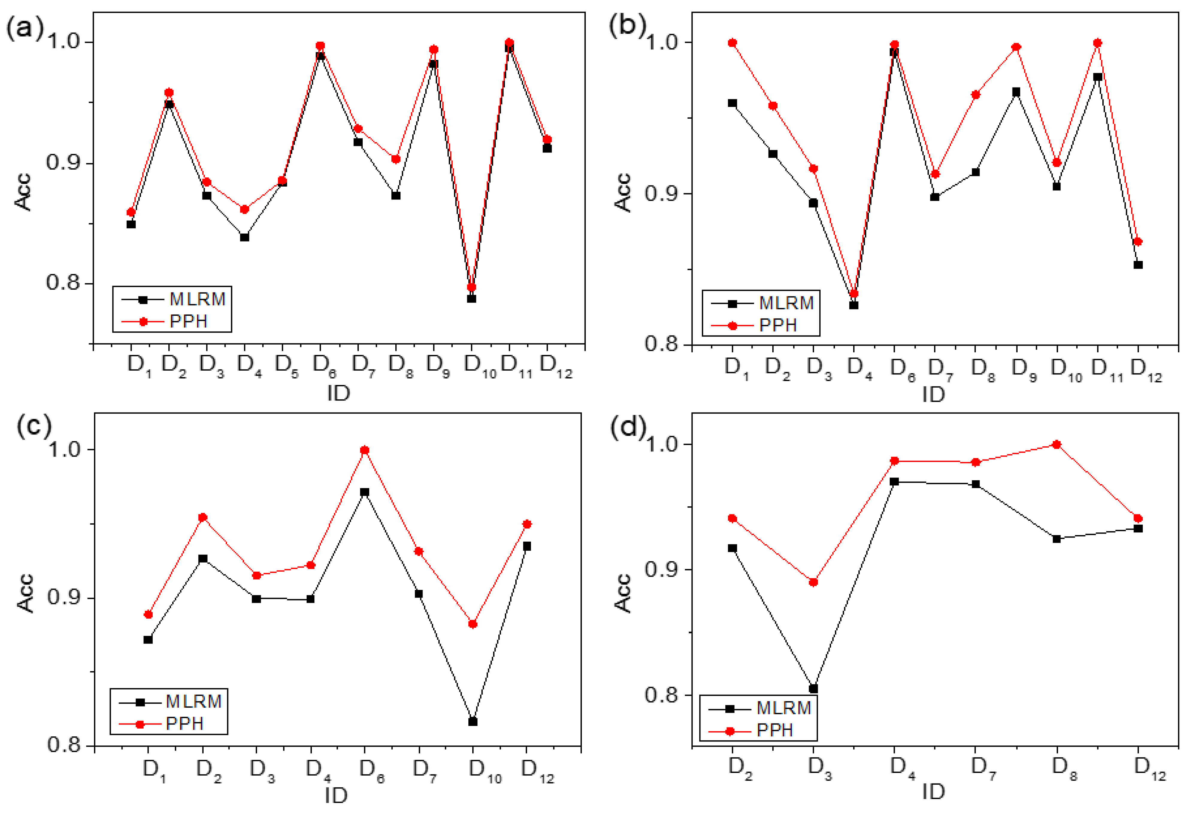
4.4. Comparison between PPH and MLRM

A PPH is proposed based on the criterion of SS and MLRM. The criterion of SS is as follows: if the $\delta$ and $\mathsf{\Omega }$ of samples are in the scope of $\delta \le 6.6\%$ and $\mathsf{\Omega }\ge 1.1$, the phases of samples are recognized as SS. To better illustrate the criterion of SS, a scatter plot based on the $\delta -\mathsf{\Omega }$ coordinate system is shown in Figure 10, which shows the distribution of SS and non-SS of HEAs. In Figure 10, the horizontal axis is $\delta \%$, and the vertical axis is $\mathsf{\Omega }$. The horizontal virtual line is $\mathsf{\Omega }=1.1$, the vertical virtual line is $\delta =6.6\%$, the upper left corner of the dotted line represents the scope of $\delta \le 6.6\%$, and $\mathsf{\Omega }\ge 1.1$. The red circle represents the samples for which the phase is SS, and the blue triangle represents the samples for which the phase is non-SS. Figure 10 shows that the phase of most samples in the upper left corner are SS in each dataset, and most samples of SS fall within the range of $\delta \le 6.6\%$ and $\mathsf{\Omega }\ge 1.1$. The experimental results show that the criterion $\delta \le 6.6\%$ and $\mathsf{\Omega }\ge 1.1$ has good effect on SS phase determination. Therefore, the criterion of SS is integrated to the PPH to improve the phase prediction accuracy of HEAs.

In order to verify the performance of the PPH, a set of comparison experiments between PPH and MLRM are carried out. The comparison of the results is shown in Figure 11. In Figure 11, the accuracies of PPH and MLRM in all, quinaries, senaries, and septenaries are shown in (a), (b), (c), and (d), respectively. The horizontal axis is the ID of these datasets, and the vertical axis is the accuracy. The red line with circles shows the accuracy of PPH. The black line with squares represents the accuracy of algorithms recommended by MLRM. As shown in Figure 11, PPH has higher prediction accuracy than MLRM in all, quinaries, senaries, and septenaries.

The specific results are listed in

Table 15. Accuracy comparison between PPH and MLRM in all, quinaries, senaries, and septenaries.

ID	All		Quinaries		Senaries		Septenaries
	MLRM	PPH	MLRM	PPH	MLRM	PPH	MLRM	PPH
D1	0.849 ± 0.008	0.859 ± 0.005	0.960 ± 0.027	1.000 ± 0.000	0.872 ± 0.006	0.889 ± 0.008	NULL	NULL
D2	0.949 ± 0.013	0.959 ± 0.007	0.927 ± 0.004	0.958 ± 0.021	0.927 ± 0.009	0.955 ± 0.014	0.918 ± 0.022	0.941 ± 0.009
D3	0.873 ± 0.003	0.884 ± 0.011	0.894 ± 0.010	0.917 ± 0.013	0.900 ± 0.013	0.915 ± 0.009	0.806 ± 0.007	0.890 ± 0.010
D4	0.838 ± 0.009	0.862 ± 0.013	0.826 ± 0.034	0.834 ± 0.016	0.899 ± 0.017	0.922 ± 0.007	0.970 ± 0.005	0.987 ± 0.005
D5	0.884 ± 0.030	0.886 ± 0.009	NULL	NULL	NULL	NULL	NULL	NULL
D6	0.989 ± 0.007	0.997 ± 0.002	0.994 ± 0.002	0.999 ± 0.001	0.972 ± 0.012	1.000 ± 0.000	NULL	NULL
D7	0.918 ± 0.010	0.929 ± 0.004	0.898 ± 0.005	0.913 ± 0.005	0.903 ± 0.002	0.932 ± 0.013	0.968 ± 0.018	0.986 ± 0.006
D8	0.873 ± 0.025	0.903 ± 0.020	0.914 ± 0.004	0.966 ± 0.004	NULL	NULL	0.925 ± 0.033	1.000 ± 0.000
D9	0.983 ± 0.010	0.994 ± 0.003	0.968 ± 0.006	0.997 ± 0.002	NULL	NULL	NULL	NULL
D10	0.787 ± 0.009	0.797 ± 0.002	0.905 ± 0.004	0.921 ± 0.012	0.817 ± 0.006	0.882 ± 0.025	NULL	NULL
D11	0.995 ± 0.002	1.000 ± 0.000	0.978 ± 0.005	1.000 ± 0.000	NULL	NULL	NULL	NULL
D12	0.912 ± 0.003	0.920 ± 0.004	0.853 ± 0.022	0.868 ± 0.011	0.935 ± 0.005	0.950 ± 0.019	0.933 ± 0.022	0.941 ± 0.008

. The first column is the ID of datasets. Column 2, column 4, column 6, and column 8 are the accuracies of MLRM in all, quinaries, senaries, and septenaries, respectively. Column 3, column 5, column 7, and column 9 are the accuracies of PPH in all, quinaries, senaries, and septenaries, respectively. NULL represents no accuracy of MLRM and PPH. From Table 15, it can be concluded that the accuracy of PPH is higher than that of MLRM. The reason could be that PPH combines the advantages of the criterion of SS and MLRM. The MLRM is a pure ML method, and it does not make full use of the professional knowledge in the material field. The criterion of SS has strong interpretability and generalization and requires only a small amount of training samples. Therefore, the prediction accuracy of PPH is higher than that of MLRM [33,34,51].

5. Conclusions

In order to predict the phases of HEAs, in this paper, we propose the phase prediction of HEAs by integrating the criterion and machine learning recommendation method. First, a meta-knowledge table based on characteristics of HEAs and performance of candidate algorithms is established, and the experiments show that meta-learning can recommend the algorithm with ideal accuracy on some datasets for material designers. Second, in order to guide material designers to select an algorithm with higher accuracy, an MLRM based on SNN and DISKR is proposed. The experimental results show that the recommendation accuracy of the MLRM is higher than that of meta-learning based on KNN on all, quinary, senary, and septenary HEAs. Third, the PPH consisting of the criterion of SS and MLRM is proposed. Compared with other ML algorithms in the HEA field, the experimental results show that the PPH can achieve performance than the traditional meta-learning method. The average prediction accuracy of the PPH in all, quinary, senary, and septenary HEAs is 91.6%, 94.3%, 93.1%, and 95.8%, respectively. The method proposed in this paper can reduce the burden of material designers in selecting algorithms, effectively improve the prediction accuracy of HEAs phase, and considerably reduce the experimental time and cost. In addition, the PPH can also provide a research foundation in other material fields.

References

1. Manzoor, A.; Pandey, S.; Chakraborty, D.; Phillpot, S.R.; Aidhy, D.S. Entropy contributions to phase stability in binary random solid solutions. NPJ Comput. Mater. 2018, 4, 1–10. [Google Scholar] [CrossRef]
2. Gorniewicz, D.; Przygucki, H.; Kopec, M.; Karczewski, K.; Jozwiak, S. TiCoCrFeMn (BCC + C14) High-Entropy Alloy Multiphase Structure Analysis Based on the Theory of Molecular Orbitals. Materials 2021, 14, 5285. [Google Scholar] [CrossRef] [PubMed]
3. Liu, L.; Paudel, R.; Liu, Y.; Zhao, X.L.; Zhu, J.C. Theoretical and Experimental Studies of the Structural, Phase Stability and Elastic Properties of AlCrTiFeNi Multi-Principle Element Alloy. Materials 2020, 13, 4353. [Google Scholar] [CrossRef] [PubMed]
4. Miracle, D.B.; Senkov, O.N. A critical review of high entropy alloys and related concepts. Acta Mater. 2017, 122, 448–511. [Google Scholar] [CrossRef] [Green Version]
5. Yang, X.; Zhang, Y. Prediction of high-entropy stabilized solid-solution in multi-component alloys. Mater. Chem. Phys. 2012, 132, 233–238. [Google Scholar] [CrossRef]
6. Senkov, O.N.; Miracle, D.B. A new thermodynamic parameter to predict formation of solid solution or intermetallic phases in high entropy alloys. J. Alloys Compd. 2016, 658, 603–607. [Google Scholar] [CrossRef] [Green Version]
7. Gao, M.C.; Zhang, C.; Gao, P.; Zhang, F.; Ouyang, L.Z.; Widom, M.; Hawk, J.A. Thermodynamics of concentrated solid solution alloys. Curr. Opin. Solid State Mater. Sci. 2017, 21, 238–251. [Google Scholar] [CrossRef]
8. Ding, Q.Q.; Zhang, Y.; Chen, X.; Fu, X.Q.; Chen, D.K.; Chen, S.J.; Gu, L.; Wei, F.; Bei, H.B.; Gao, Y.F.; et al. Tuning element distribution, structure and properties by composition in high-entropy alloys. Nature 2019, 574, 223–227. [Google Scholar] [CrossRef]
9. Li, Z.M.; Pradeep, K.G.; Deng, Y.; Raabe, D.; Tasan, C.C. Metastable high-entropy dual-phase alloys overcome the strength-ductility trade-off. Nature 2016, 534, 227–230. [Google Scholar] [CrossRef]
10. Ye, Y.F.; Wang, Q.; Lu, J.; Liu, C.T.; Yang, Y. High-entropy alloy: Challenges and prospects. Mater. Today 2016, 19, 349–362. [Google Scholar] [CrossRef]
11. Zhang, Y.; Yang, X.; Liaw, P.K. Alloy Design and Properties Optimization of High-Entropy Alloys. JOM 2012, 64, 830–838. [Google Scholar] [CrossRef]
12. Guo, S.; Liu, C.T. Phase stability in high entropy alloys: Formation of solid-solution phase or amorphous phase. Prog. Nat. Sci. Mater. Int. 2011, 21, 433–446. [Google Scholar] [CrossRef] [Green Version]
13. Tan, Y.M.; Li, J.S.; Tang, Z.W.; Wang, J.; Kou, H.C. Design of high-entropy alloys with a single solid-solution phase: Average properties vs. their variances. J. Alloys Compd. 2018, 742, 430–441. [Google Scholar] [CrossRef]
14. Dai, D.B.; Xu, T.; Wei, X.; Ding, G.T.; Xu, Y.; Zhang, J.C.; Zhang, H.R. Using machine learning and feature engineering to characterize limited material datasets of high-entropy alloys. Comput. Mater. Sci. 2020, 175, 1–6. [Google Scholar] [CrossRef]
15. Zhou, Z.; Zhou, Y.; He, Q.; Ding, Z.; Li, F.; Yang, Y. Machine learning guided appraisal and exploration of phase design for high entropy alloys. NPJ Comput. Mater. 2019, 5, 1–9. [Google Scholar] [CrossRef] [Green Version]
16. Pei, Z.; Yin, J.; Hawk, J.A.; Alman, D.E.; Gao, M.C. Machine-learning informed prediction of high-entropy solid solution formation: Beyond the Hume-Rothery rules. NPJ Comput. Mater. 2020, 6, 1–8. [Google Scholar] [CrossRef]
17. Klimenko, D.; Stepanov, N.; Li, J.; Fang, Q.; Zherebtsov, S. Machine Learning-Based Strength Prediction for Refractory High-Entropy Alloys of the Al-Cr-Nb-Ti-V-Zr System. Materials 2021, 14, 7213. [Google Scholar] [CrossRef]
18. Dai, W.; Zhang, L.; Fu, J.; Chai, T.; Ma, X. Dual-Rate Adaptive Optimal Tracking Control for Dense Medium Separation Process Using Neural Networks. IEEE Trans. Neural Netw. Learn. Syst. 2021, 32, 4202–4216. [Google Scholar] [CrossRef]
19. Islam, N.; Huang, W.J.; Zhuang, H.L.L. Machine learning for phase selection in multi-principal element alloys. Comput. Mater. Sci. 2018, 150, 230–235. [Google Scholar] [CrossRef]
20. Huang, W.J.; Martin, P.; Zhuang, H.L.L. Machine-learning phase prediction of high-entropy alloys. Acta Mater. 2019, 169, 225–236. [Google Scholar] [CrossRef]
21. Qu, N.; Chen, Y.C.; Lai, Z.H.; Liu, Y.; Zhu, J.C. The phase selection via machine learning in high entropy alloys. Procedia Manuf. 2019, 37, 299–305. [Google Scholar] [CrossRef]
22. Liu, H.; Chen, J.; Hissel, D.; Su, H. Remaining useful life estimation for proton exchange membrane fuel cells using a hybrid method. Appl. Energy 2019, 237, 910–919. [Google Scholar] [CrossRef]
23. Wolpert, D.H.; Macready, W.G. No Free Lunch Theorems for Search. IEEE Trans. Evol. Comput. 1997, 1, 67–82. [Google Scholar] [CrossRef] [Green Version]
24. Khan, I.; Zhang, X.C.; Rehman, M.; Ali, R. A Literature Survey and Empirical Study of Meta-Learning for Classifier Selection. IEEE Access 2020, 8, 10262–10281. [Google Scholar] [CrossRef]
25. Aguiar, G.J.; Mantovani, R.G.; Mastelini, S.M.; de Carvalho, A.C.P.F.L.; Campos, G.F.C.; Junior, S.B. A meta-learning approach for selecting image segmentation algorithm. Pattern Recognit. Lett. 2019, 128, 480–487. [Google Scholar] [CrossRef]
26. Chu, X.H.; Cai, F.L.; Cui, C.; Hu, M.Q.; Li, L.; Qin, Q.D. Adaptive recommendation model using meta-learning for population-based algorithms. Inf. Sci. 2019, 476, 192–210. [Google Scholar] [CrossRef]
27. Cui, C.; Hu, M.Q.; Weir, J.D.; Wu, T. A recommendation system for meta-modeling: A meta-learning based approach. Expert Syst. Appl. 2016, 46, 33–44. [Google Scholar] [CrossRef] [Green Version]
28. Pimentel, B.A.; de Carvalho, A.C.P.L.F. A new data characterization for selecting clustering algorithms using meta-learning. Inf. Sci. 2019, 477, 203–219. [Google Scholar] [CrossRef]
29. Ferrari, D.G.; de Castro, L.N. Clustering algorithm selection by meta-learning systems: A new distance-based problem characterization and ranking combination methods. Inf. Sci. 2015, 301, 181–194. [Google Scholar] [CrossRef]
30. Song, Y.S.; Liang, J.Y.; Lu, J.; Zhao, X.W. An efficient instance selection algorithm for k nearest neighbor regression. Neurocomputing 2017, 251, 26–34. [Google Scholar] [CrossRef]
31. Zhang, S.C. Shell-neighbor method and its application in missing data imputation. Appl. Intell. 2010, 35, 123–133. [Google Scholar] [CrossRef]
32. Lv, W.; Mao, Z.Z.; Yuan, P.; Jia, M.X. Multi-kernel learnt partial linear regularization network and its application to predict the liquid steel temperature in ladle furnace. Knowl. Based Syst. 2012, 36, 280–287. [Google Scholar] [CrossRef]
33. Lv, W.; Mao, Z.Z.; Yuan, P.; Jia, M.X. Pruned Bagging Aggregated Hybrid Prediction Models for Forecasting the Steel Temperature in Ladle Furnace. Steel Res. Int. 2014, 85, 405–414. [Google Scholar] [CrossRef]
34. Hou, S.; Liu, J.H.; Lv, W. Flotation Height Prediction under Stable and Vibration States in Air Cushion Furnace Based on Hard Division Method. Math. Probl. Eng. 2019, 2019, 1–14. [Google Scholar] [CrossRef] [Green Version]
35. Chang, X.J.; Zeng, M.Q.; Liu, K.L.; Fu, L. Phase Engineering of High-Entropy Alloys. Adv. Mater. 2020, 32, 1–22. [Google Scholar] [CrossRef]
36. Lemke, C.; Budka, M.; Gabrys, B. Metalearning: A survey of trends and technologies. Artif. Intell. Rev. 2015, 44, 117–130. [Google Scholar] [CrossRef] [Green Version]
37. Arjmand, A.; Samizadeh, R.; Dehghani Saryazdi, M. Meta-learning in multivariate load demand forecasting with exogenous meta-features. Energy Effic. 2020, 13, 871–887. [Google Scholar] [CrossRef]
38. Smith-Miles, K.A. Cross-disciplinary perspectives on meta-learning for algorithm selection. ACM Comput. Surv. 2009, 41, 1–25. [Google Scholar] [CrossRef]
39. Zhang, S.C. Parimputation: From Imputation and Null-Imputation to Partially Imputation. IEEE Intell. Inform. Bull. 2008, 9, 32–38. [Google Scholar]
40. Liu, H.W.; Wu, X.D.; Zhang, S.C. Neighbor selection for multilabel classification. Neurocomputing 2016, 182, 187–196. [Google Scholar] [CrossRef]
41. Zhang, Y.; Wen, C.; Wang, C.X.; Antonov, S.; Xue, D.Z.; Bai, Y.; Su, Y.J. Phase prediction in high entropy alloys with a rational selection of materials descriptors and machine learning models. Acta Mater. 2020, 185, 528–539. [Google Scholar] [CrossRef]
42. Tamal, M.; Alshammari, M.; Alabdullah, M.; Hourani, R.; Alola, H.A.; Hegazi, T.M. An integrated framework with machine learning and radiomics for accurate and rapid early diagnosis of COVID-19 from Chest X-ray. Expert Syst. Appl. 2021, 180, 1–8. [Google Scholar] [CrossRef] [PubMed]
43. Wani, M.A.; Roy, K.K. Development and validation of consensus machine learning-based models for the prediction of novel small molecules as potential anti-tubercular agents. Mol. Divers. 2021, 1–12. [Google Scholar] [CrossRef]
44. Toda-Caraballo, I.; Rivera-Díaz-del-Castillo, P.E.J. A criterion for the formation of high entropy alloys based on lattice distortion. Intermetallics 2016, 71, 76–87. [Google Scholar] [CrossRef]
45. Leong, Z.Y.; Huang, Y.H.; Goodall, R.; Todd, I. Electronegativity and enthalpy of mixing biplots for High Entropy Alloy solid solution prediction. Mater. Chem. Phys. 2018, 210, 259–268. [Google Scholar] [CrossRef]
46. Poletti, M.G.; Battezzati, L. Electronic and thermodynamic criteria for the occurrence of high entropy alloys in metallic systems. Acta Mater. 2014, 75, 297–306. [Google Scholar] [CrossRef]
47. King, D.J.M.; Middleburgh, S.C.; McGregor, A.G.; Cortie, M.B. Predicting the formation and stability of single phase high-entropy alloys. Acta Mater. 2016, 104, 172–179. [Google Scholar] [CrossRef]
48. Andreoli, A.F.; Orava, J.; Liaw, P.K.; Weber, H.; de Oliveira, M.F.; Nielsch, K.; Kaban, I. The elastic-strain energy criterion of phase formation for complex concentrated alloys. Materialia 2019, 5, 1–12. [Google Scholar] [CrossRef]
49. Peng, Y.T.; Zhou, C.Y.; Lin, P.; Wen, D.Y.; Wang, X.D.; Zhong, X.Z.; Pan, D.H.; Que, Q.; Li, X.; Chen, L.; et al. Preoperative Ultrasound Radiomics Signatures for Noninvasive Evaluation of Biological Characteristics of Intrahepatic Cholangiocarcinoma. Acad. Radiol. 2020, 27, 785–797. [Google Scholar] [CrossRef]
50. Jung, Y. Multiple predicting K-fold cross-validation for model selection. J. Nonparametr. Stat. 2017, 30, 197–215. [Google Scholar] [CrossRef]
51. Hou, S.; Zhang, X.; Dai, W.; Han, X.; Hua, F. Multi-Model- and Soft-Transition-Based Height Soft Sensor for an Air Cushion Furnace. Sensors 2020, 20, 926. [Google Scholar] [CrossRef] [PubMed] [Green Version]
Figure 1. Schematic diagram of meta-learning.
Materials 15 03321 g001
Figure 2. SNN of the query instance.
Materials 15 03321 g002
Figure 3. Schematic diagram of MLRM.
Materials 15 03321 g003
Figure 4. Schematic diagram of phase prediction frame of HEAs.
Materials 15 03321 g004
Figure 5. Quantity of SS, IM, SS+IM, and AM in the quinaries, senaries, and septenaries. (a) D1, (b) D2, (c) D3, (d) D4, (e) D5, (f) D6, (g) D7, (h) D8, (i) D9, (j) D10, (k) D11, and (l) D12.
Materials 15 03321 g005
Figure 6. Statistics of the occurrence time of each element in 12 datasets. (a) D1, (b) D2, (c) D3, (d) D4, (e) D5, (f) D6, (g) D7, (h) D8, (i) D9, (j) D10, (k) D11, (l) D12.
Materials 15 03321 g006
Figure 7. Heatmap of Pearson correlation coefficient matrix among 5 parameters in 12 datasets.
Materials 15 03321 g007
Figure 8. Accuracy comparison between meta-learning and traditional ML algorithms. (a) all, (b) quinaries, (c) senaries, and (d) septenaries.
Materials 15 03321 g008
Figure 9. Accuracy comparison between MLRM and meta-learning. (a) all, (b) quinaries, (c) senaries, and (d) septenaries.
Materials 15 03321 g009
Figure 10. Scatter plot based on the δ Ω coordinate system. (a) D1, (b) D2, (c) D3, (d) D4, (e) D5, (f) D6, (g) D7, (h) D8, (i) D9, (j) D10, (k) D11, (l) D12.
Materials 15 03321 g010
Figure 11. Accuracy comparison between PPH and MLRM. (a) all, (b) quinaries, (c) senaries, and (d) septenaries.
Materials 15 03321 g011